Abstract
In this article, we discuss the relationship and transition between self- and Fick diffusion coefficients in continuous implicit solvents across different particle densities. By applying the established expressions for self-diffusion and Fick diffusion coefficients in binary solutions, we analyze how the local environment influences diffusion through thermodynamic factors, which can be readily evaluated within the framework of Kirkwood–Buff (KB) theory. These thermodynamic factors, originally defined as derivatives of thermodynamic activity, vary with changes in local particle densities, particularly in the presence of aggregation effects. Consequently, the transition from self- to Fick diffusion coefficients can be understood as a reflection of variations in these thermodynamic factors. Langevin Dynamics simulations at low number densities show excellent agreement with the analytical expressions derived. Overall, our findings provide deeper insight into how local structural environments shape particle dynamics, clarifying the connection between KB theory and the transition from self- to Fick diffusion coefficients.
1. Introduction
Understanding diffusive motion is of fundamental importance for many technical applications. Almost all chemical separation processes such as distillation, absorption, extraction, or condensation are based on the transport of substances within a liquid mixture or across a phase boundary [1,2]. The corresponding diffusion processes are often the rate-determining step for such separation mechanisms, which is why optimizing these processes also requires a fundamental understanding of the governing principles. Given their importance in chemical and industrial applications, extensive research has focused on the diffusive behavior of various solvent mixtures [3,4,5,6], employing both numerical and experimental approaches [7,8,9,10,11,12,13,14,15,16,17,18,19,20,21,22,23,24]. In general, one can distinguish between self-diffusion and collective or transport diffusion of particles. In contrast to self-diffusion of isolated single tracer particles, transport diffusion in terms of Fick or Maxwell–Stefan diffusion processes can be regarded as a collective transport mechanism due to correlations between the components of a solution [4,5,6,19,23,24,25].
Whereas self-diffusion of tracer particles can be studied experimentally via advanced NMR measurements or microscopic techniques [26], the investigation of transport diffusion by Raman spectroscopy, diaphragm cell techniques, interferometry, microfluidics, or quasi-elastic neutron scattering experiments is far more complicated [19,25]. Moreover, the individual diffusion coefficients for components in binary mixtures often reveal significant deviations from Fick diffusion coefficients, such that the introduction of effective diffusion coefficients, even in non-porous environments, becomes obligatory [25]. Thus, most of the previous works on diffusive motion rely on the evaluation of tracer diffusion, which ignores the presence of other molecules [19].
However, these simplifications are often not really expedient, as molecular correlations often play an important role in the dynamics of liquids [27,28]. A prominent example are correlations in electrolyte solutions and their influence on the dynamic behavior and the resulting charge transport [26,29]. A key example of this is the crucial limiting of transport processes due to the formation of ion pairs [29,30,31,32,33,34,35,36,37,38]. This formation has been shown, for example, to significantly reduce ionic conductivity [29,32,39,40,41,42]. Similarly, the role of local structures on diffusion processes is, in many cases, not yet fully understood. However, in the last few years, some works linking the thermodynamic factors and the local environment within the framework of Kirkwood–Buff (KB) integrals have provided some new insights [17,19,22,23,24,43]. Accordingly, it was shown that Maxwell–Stefan and Fick diffusion coefficients can be effectively calculated via consideration of the derivative of the thermodynamic activity in the framework of the KB theory [17,19,22,23,24,43,44,45,46,47,48,49,50]. Thus far, the corresponding simulations and expressions have only been evaluated for collective diffusion, whereby self-diffusion has not yet been taken into account. However, molecular self-diffusion is of utmost relevance for a number of processes, including diffusion in nanopores, confined geometries, and crowded solutions. Accordingly, the transition from self- to collective diffusion based on the insights gained from understanding the influence of the local environment through the description of expressions from KB theory is of great interest [50,51,52,53,54].
In addition, many simulation approaches rely on implicit solvents [55,56], where only one component of the solution, often the main solute, is considered for reasons of computational efficiency. Accordingly, the relationship between self- and collective transport diffusion coefficients is not fully defined in these simulations [57,58,59]. For low particle densities, for example, it was reported that the self-diffusion coefficients change linearly with density variations [57,60,61,62]. Here, explicit reference was made to self-diffusion coefficients, whereby the collective diffusion coefficients were not taken into account.
In this article, we present expressions for the transition of self-diffusion coefficients into Fick diffusion coefficients for increasing particle densities. We show that the local environmental structure in terms of KB integrals as well as the corresponding derivative of the thermodynamic activity crucially influence diffusive behavior. Our expressions are validated by Langevin Dynamics (LD) simulations, which allow us a detailed comparison with the analytical findings. Accordingly, our results reveal that previous empirical relations in terms of linearly varying self-diffusion coefficients upon number density variation can be simply regarded as transitions from self- to Fick diffusion coefficients by means of thermodynamic factor changes.
The article is organized as follows. In the Section 2, we present the theoretical background of our approach in combination with the corresponding expressions. In the Section 3, we discuss the details of the simulations. All computational results are presented in the Section 4. We conclude with a summary in the Section 5.
2. Theoretical Background
In the following subsection, we will first give some general background information on the thermodynamic relations for diffusive motion. The corresponding results are important for discussing the relationship between Fick and self-diffusion coefficients in terms of thermodynamic factors. In the second subsection, we will show how the thermodynamic factor can be calculated using KB theory.
2.1. Basic Thermodynamics: Diffusive Motion
As a starting point, the fundamental equation of entropy production for a non-equilibrium system reads
in which and represent generalized thermodynamic forces and fluxes, respectively. As it was often discussed in detail elsewhere [6,63], the thermodynamic fluxes can also be expressed by
where represent the phenomenological Onsager coefficients, such that Equation (1) can be written as [6]
in order to include all irreversible processes that contribute to the entropy production of the system. For the following discussion, we omit vector notation for reasons of clarity. In regards of a constant temperature T, a constant pressure p, and in absence of any external potential fields and chemical reactions with and thus , the entropy production of a system with C components reads [63]
with mass fluxes of the individual species and the chemical potential . With regard to conservation of mass and momentum, it follows , and Equation (4) can be rewritten as
in accordance with . Specifically for a binary mixture () with components and , the entropy production in Equation (5) under the requirement reads
such that, in accordance with a linear force-flux relation (Equation (3)), the corresponding entropy production and thermodynamic mass flux at constant temperature can be identified as
and
with . The gradient in Equation (8) can be further simplified in terms of the following relation for the mole fractions
and in combination with the general Gibbs–Duhem relation [64]
according to for a binary mixture, which yields
with the number density and the total bulk number density , including molecules of species in volume V for insertion into Equation (8). With regard to its dependencies, the total derivative of the chemical potential at constant pressure and temperature can be written as
such that the resulting relation after combination with Equation (11) reads
which gives
after insertion into Equation (8).
Accordingly, one can define the Fick diffusion coefficient
which can be transformed into [45]
with the partial molar volume , yielding
by using the identity [45] . A combination of the identity with Equations (14) and (17) finally provides the expression
including the definition of the thermodynamic factor [23,24,65]
which is also valid for with regard to reasons of symmetry and vanishing mass flux for a two-component system.
2.2. Diffusion Coefficients, Thermodynamic Factors, and KB Theory
As a standard approach for the description of correlated diffusive motion of molecules in a mixture, the molar flux of component in a solution with C components can be written by the generalized Fick law [4,19]
with the total bulk number density , including molecules of species in volume V. As can be seen, the mass flux depends on the gradient of the mole fraction and is proportional to the Fick diffusion coefficients with . It is important to note that Equation (20) represents the formal definition of the Fick diffusion coefficient in terms of the generalized Fick law for constant volume conditions, where the molar flux is proportional to the gradient of the mole fraction. In contrast, Equation (14) is derived from the thermodynamic framework for conditions and relates the diffusion coefficient to Onsager coefficients and the derivative of the chemical potential. Whereas Equation (14) involves the derivative of the chemical potential with respect to the number density, Equation (20) is based on the derivative of the mole fraction. Accordingly, Equation (14) should be regarded as a specific thermodynamic relation, while Equation (20) provides the general formal definition. Both formulations are consistent within their respective frameworks and highlight the connection between transport processes and thermodynamic factors.
For binary mixtures with components and with regard to momentum conservation in terms of , it follows for Equation (20) that only one identical Fick diffusion coefficient for both components exists [5,19,25]. This Fick diffusion coefficient in Equation (20) then reduces to
by way of symmetry. After comparison with Equation (18), it follows that the Fick diffusion coefficient can also be written as
which highlights the influence of the thermodynamic factor. Noteworthy, for low densities of component in binary mixtures, the Fick and self-diffusion coefficients become identical in accordance with the relation
with self-diffusion coefficient [17,19,22]. In terms of a more detailed interpretation, thermodynamic factors account for the non-ideality of the solution, and thus provide a connection between transport mechanisms and thermodynamics. Notably, non-ideal effects are evident for all values as for most real solutions, which highlights their potential importance for diffusive processes. In accordance with the relation
one can insert the basic definition of the chemical potential
with the thermodynamic activity into Equation (24), leading to
with the derivative of the thermodynamic activity
For a binary solution, this expression can also be written in the framework of KB theory [29,45,46,47] according to
with the KB integrals
including the radial distribution function . In consequence, the thermodynamic factor can be identified as the derivative of the thermodynamic activity , such that Equation (22) reads
which already highlights the integral importance of the local environment on the diffusion process in terms of the KB integrals. A more detailed derivation of the KB expression can be found in Appendix A.
2.3. Self-Diffusion Coefficients and Computer Simulations
In terms of Equations (22) and (23), one can already notice that
which results in
for low number densities and nearly ideal solutions, leading to the following expression
for the self-diffusion coefficients. From further analytic considerations, one can also compute the true self-diffusion coefficient for stochastic dynamics simulations [66] in terms of
with the mass of the particle m and the friction coefficient . The corresponding values can be compared to the self-diffusion coefficient for a single and isolated particle in computer simulations in terms of velocity autocorrelation functions or the mean-square displacement [67]. For reliable simulation protocols, one can conclude that and hence assume that
where accounts for the center-of-mass diffusion and higher-order correlation effects, which are absent for one particle. In our LD simulations, the center-of-mass diffusion coefficient also arises as an additive correction required to conserve momentum. While is negligible in most systems, in the implicit solvent representation, it assumes a finite value and must be explicitly considered. Specifically, finite simulations may exhibit a net drift or center-of-mass translation of the entire system, which is not captured by the mean-square displacement of individual particles. Moreover, hydrodynamic correlations in the explicit solvent, which are absent in our simulations, could couple particle motion to collective flow fields, thereby enhancing center-of-mass diffusion. We also note that finite-size effects under periodic boundary conditions can introduce artifacts, as the center-of-mass motion is constrained by box size and thermostat coupling. Finally, collective relaxation modes, contribute additional transport channels that manifest in . Hence, one would expect deviations from the mesured self-diffusion coefficient and the analytical result from Equation (34) for and for increasing particle densities. Despite these higher-order effects, one can conclude that the self-diffusion coefficient, even in implicit solvent simulations, depends on the Fick diffusion coefficient and thus depends on non-ideal and colligative effects. Comparable assumptions and observations were also previously discussed in Ref. [57], where the diffusion coefficients were described by
where is the area fraction, is the diffusion coefficient at infinite dilution and thus the self-diffusion coefficient, and is a numerical factor that depends on the nature of interactions.
3. Simulation Details
We performed Langevin Dynamics (LD) simulations for a varying amount of single particles in a continuum implicit solvent. The systems were simulated with the GROMACS 5.0.2 software package [68,69,70]. The spherical particles were modified from the GROMOS 43a1 force field [71], where the corresponding mass of the particles was set identical to sodium ions Na+ (atom type ‘NA’) while the Lennard–Jones interaction parameters were taken from Zn2+ ions (atom type ‘ZN2+’). In addition, the charge was set to zero. The smaller mass of sodium was chosen to achieve an efficient sampling of the phase space for the given time scale. In addition, slight attractive dispersion interactions as represented by the Lennard–Jones parameters from the Zn2+ ions enforce weak particle interactions and accumulation.
A leap-frog stochastic dynamics integrator [72] was used to reproduce the stochastic motion of the particles. The equation of motion reads
with the mass of a particle i fom the chosen species, the velocity , the conservative forces , and the random force . The random force obeys the conditions of Gaussian white noise in terms of
in combination with . The temperature was set to K in all runs and the friction coefficient was chosen as ps−1. Accordingly, the self-diffusion coefficient from Equation (34) is cm2/s. We used NVT and periodic boundary conditions in all directions for a fixed cubic box length of in order to avoid varying finite-size effects [73]. Random insertion of , and 44 spherical particles for the individual simulations resulted in different number densities ranging from nm−3. Each system was simulated for 50 ns, with a time step of Δt = 2 fs and the first 2 ns were used for equilibration. For the uncharged spherical particles, all Coulomb interactions were switched off. The radial distribution functions were calculated by
where denotes the average number density of particles around particles in the system. The term represents the average number of particles around particles found within a spherical shell of thickness at a distance r from a reference particle. Due to finite box sizes, we introduced a correction scheme [43,74] for the calculation of KB integrals (Equation (29)) in terms of
with [50]. Accordingly, the corresponding KB integrals for the calculation of in Equation (28) were also calculated with the expressions from Equation (40).
4. Results
4.1. Structural and Thermodynamic Properties
In the following, we denote all solute particles with the subscript “1”, while the continuum phantom solvent is denoted with the subscript ’2’ for reasons of clarity. The radial distribution functions for chosen particle densities are presented in Figure 1.
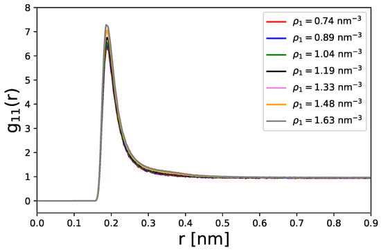
Figure 1.
Center-of-mass radial distribution functions for different densities of spherical particles.
As can be seen, the particles reveal a pronounced short-range ordering as reflected by the high peak values at nm. This local ordering can be attributed to the attractive part of the Lennard–Jones potential, which induces slight accumulation effects in terms of first-contact shells. In accordance, one can recognize a steep decrease in the radial distribution functions with a convergence to at distances nm, which highights the transition from local to bulk regions. At particle densities of nm−3, the formation of a slight shoulder between nm can be identified, which indicates the formation of larger or even second-order contact pair shells. In summary, one can conclude that the particles show slight accumulation effects due to attractive Lennard–Jones potentials.
These effects are also evident in terms of the potential of mean force [75] according to
with the Boltzmann constant as shown in Figure 2. The PMF curves closely match the analytical Lennard–Jones interaction energies for the given parameters. This shows that both the particle interactions and the radial distribution function are governed solely by the empirical Lennard–Jones potential.
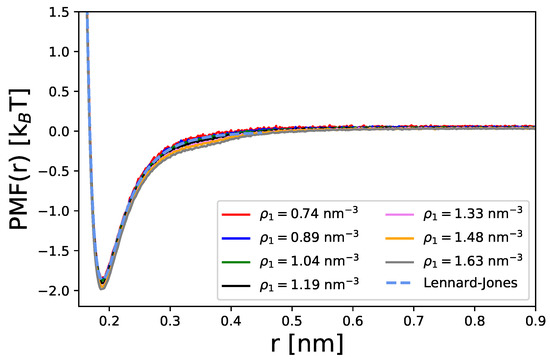
Figure 2.
Potentials of mean force calculated from Equation (41) for different densities of spherical particles. The blue dashed line is the analytic result for the Lennard-Jones potential for interactions between two particles.
Despite the large variation in particle densities, it becomes obvious that the potential of mean forces is largely comparable, with differences in the maximum values around ΔPMF . Moreover, it can be seen that these forces are attractive on length scales up to 0.55 nm with a maximum value of PMF at nm. The corresponding findings highlight that accumulation is driven by attractive Lennard–Jones interactions whose values allow for a proper binding and unbinding equilibrium. According to the rather low energy barriers, the particles are free to move in the simulation box with a moderate tendency for accumulation.
Such findings are also evident with regard to the running KB integrals (Equation (29)) as shown in the top panel of Figure 3. The corresponding converged values are shown in the bottom panel.
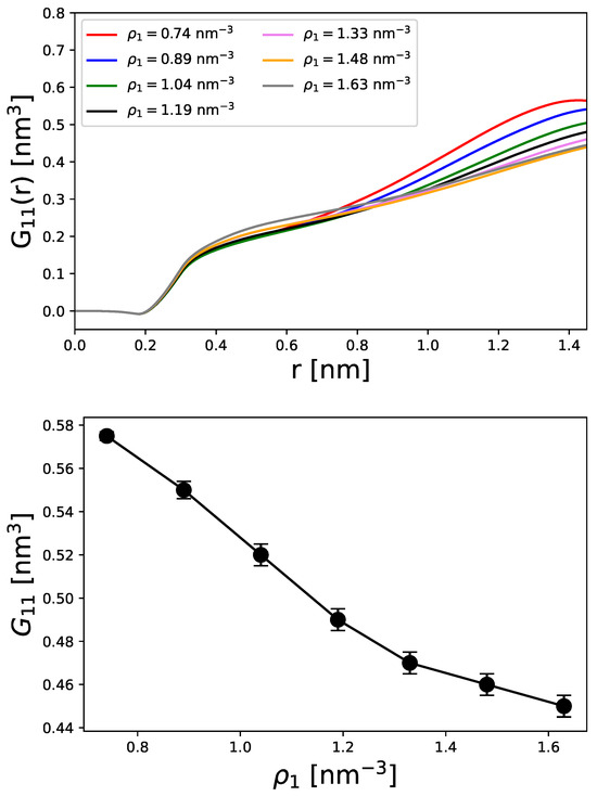
Figure 3.
Running KB integrals from Equation (40) (top panel) and converged values for at (bottom panel) for different representative densities of spherical particles. The error bars denote the standard devations of the last 5 points around the converged values.
In general, KB integrals can be interpreted as excess volumes relative to the ideal state [48]. Accordingly, all KB integrals show a slight decrease at short distances nm due to excluded volume effects. A rapid increase in the KB integrals can be observed between nm, which corresponds to the first contact pair in agreement with Figure 1. For larger distances than nm, the KB integrals finally converge to a constant value as defined by Equation (29) and shown in the bottom panel of Figure 3. With reference to Figure 3, the corresponding values of are ordered as a function of the particle density. This means that higher particle densities lead to smaller KB integrals. Such findings are consistent with the accumulation effects already observed. Since KB integrals represent the deviation from an ideal state, it can be concluded that higher particle densities deviate more strongly from a homogeneous distribution.
Comparable findings can also be observed for the preferential binding coefficients and the derivatives of the thermodynamic activity as shown in Figure 4. The preferential binding coefficient defined by [48,49]
allows us to estimate the tendency of the aggregation effects. For positive values, we can identify a preferential binding mechanism, and for negative values, a preferential exclusion effect [29,48,49]. As can be seen, the second KB integral denotes the interaction between the particles and the implicit continuum solvent. In general, implicit solvents lead to radial distribution functions , so that (Equation (29)), and thus lead to the result
whose values are shown in the top panel of Figure 4. It is clear that the converged values for distances larger than nm are positive and show a strong ordering in the densities nm−3. Accordingly, one can assume that the strength of the preferential binding mechanism increases monotoneously with increasing particles densities. The largest preferential binding coefficient can be observed for the highest particle density, which also reveals the strongest accumulation effect.
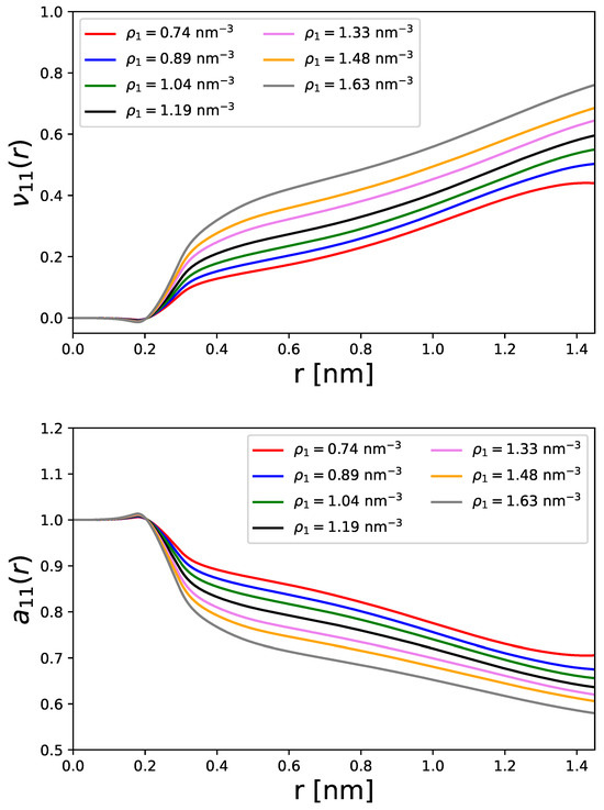
Figure 4.
Running preferential binding coefficient (top panel) and derivative of the thermodynamic activity (bottom panel) for different particle densities in a cubic simulation box of constant length.
In accordance with Equation (42), the derivative of the thermodynamic activity (Equation (28)), can also be written as
which highlights the pronounced influence of the local structure in terms of accumulation effects for the derivative of the thermodynamic activity. With regard to the conditions in our simulations, the corresponding expression reads
as was recently demonstrated in Ref. [76]. For our given conditions , the previous relation further reduces to
which is equivalent to Equation (44).
The corresponding results for the derivatives of the thermodynamic activity are shown in the bottom panel of Figure 4. The converged values are between , which highlights minimal or even moderate differences to the ideal or homogeneous state as denoted by . Lower values of are related to higher particle densities, which shows the influence of accumulation effects in comparison to the ideal distribution. One can thus clearly see that the local structure in terms of surrounding particles strongly affect the derivatives of the thermodynamic acitivity with regard to non-ideal and inhomogeneous distributions.
4.2. Dynamic Properties and Diffusive Motion
The corresponding dynamic properties are studied by the mean-square displacement (MSD) for the particles as defined by
with the position of particle i at different times, t and , and the self-diffusion coefficient . The efficient evaluation of the corresponding values over long particle trajectories can be achieved by the methods outlined in Ref. [77]. All results for the MSDs with regard to different particle densities are shown in the top panel of Figure 5.
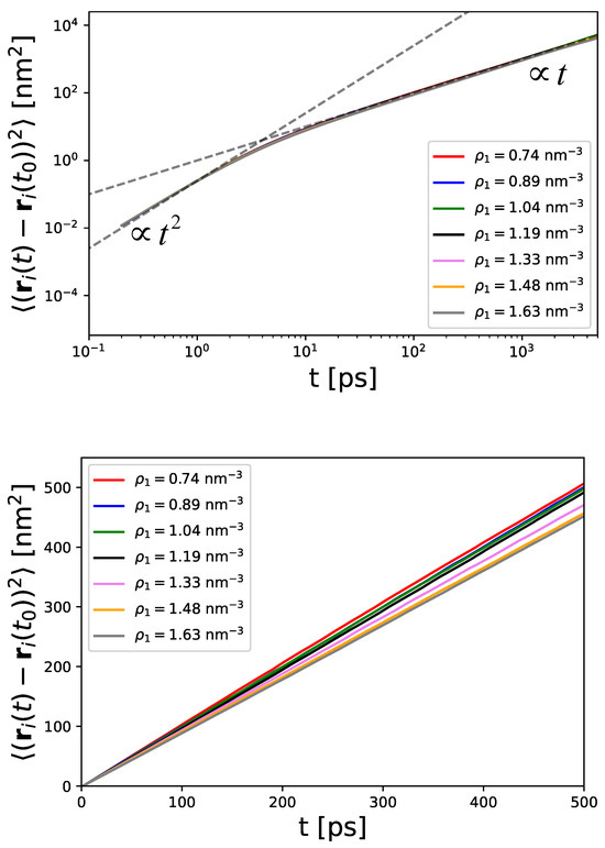
Figure 5.
Mean-square displacement of particles at different densities in a log–log plot (top panel) and in linear representation (bottom panel).
The corresponding representation in a log–log plot shows the presence of two regimes, which are known as ballistic and diffusive regimes [78,79]. The ballistic regime scales with , which can be attributed to the initial motion of particles for short times. This finding is also important for LD simulations (Equation (37)), as the mass is not neglected in contrast to Brownian Dynamics simulations. For later times, the particles usually follow the diffusive regime, which is characterized by Equation (47) and thus a linear scaling with time . It can clearly be observed that all particle densities have a comparable transition time between ps, where the diffusive motion dominates for longer times. The coincidence of these values highlights the non-existent correlations between the particles, so that the transition time depends only on the mass and the friction coefficient. Further evaluation of the MSDs for different particle densities is shown in the bottom panel of Figure 5. One can notice that the MSDs decrease for increasing particle densities.
The corresponding values for the self-diffusion coefficients from the simulations in reference to the relation for according to Equations (24) and (35) are presented in Figure 6.
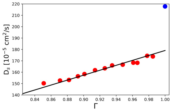
Figure 6.
Self-diffusion coefficients computed from LD simulations in terms of Equation (47) for increasing particle densities with reference to the thermodynamic factor (red circles). The corresponding black line shows the results of a linear fit in accordance with Equation (35) with fit value cm2/s and a constant value cm2/s. The correlation coefficient reads . The blue filled circle denotes the corresponding value for a single particle with and by definition.
The black solid line depicts a linear regression in agreement with Equation (35) for a constant value cm2/s with fit value cm2/s. The correlation coefficient reads with the observed , calculated , and mean values of the N diffusion coefficients. Accordingly, the corresponding self-diffusion coefficients scale with the derivative of the thermodynamic activity in agreement with Equation (35). In addition, the analytic result of Equation (34) with cm2/s is in good agreement with the corresponding data point at (blue sphere) in Figure 6, which corresponds to the evaluation of the diffusion coefficient for a single particle with .
5. Conclusions
We have studied the self-diffusion of spherical tracer particles at different number densities in an implicit solvent using LD simulations. In addition, we have also derived an analytical expression for self-diffusion coefficients, based, in particular, on an interpretation of the thermodynamic factor in the framework of KB theory. The results of the simulations are in very good agreement with the analytical expressions, which proves the validity of our considerations. Accordingly, we were able to show that a varying particle density is accompanied by a change in the self-diffusion coefficients, which is caused by a change in the derivatives of the thermodynamic activity. However, since thermodynamic activity is significantly influenced by deviations from the ideal behavior, it can be seen that local accumulation effects and thus the structure of the local environment have a decisive influence on the diffusive properties of the particles. These findings show that the common calculation of self-diffusion coefficients from computer simulations strongly depends on the local density and further aggregation effects.
As shown in previous publications [45,47,48], the derivatives of the thermodynamic activity can be expressed by KB integrals for which the integration of the corresponding radial distribution functions allows the estimation of the excess volumes. If the particle densities are low and a homogeneous continuum solvent is assumed, which is often the case for stochastic descriptions of particle motion, the corresponding KB integrals can be reduced to simple expressions.
Accordingly, the derivatives of the thermodynamic activity can be interpreted as an effective mean field, which defines the deviation from the ideality of the distribution in the local environment. If the distribution is ideal, the diffusion coefficients are not affected. When accumulation effects lead to local non-homogeneities, they alter the surrounding environment and thereby affect the diffusion coefficients. These changes are not solely due to correlation effects; the mere presence of additional particles can play a significant role. Such findings highlight a deeper link between Fick and self-diffusion coefficients, even in simple LD simulations including continuum implicit solvents. Accordingly, the analytical self-diffusion coefficient can only be estimated at and strictly for , which is often not the case.
In contrast to explicit solvent studies where Onsager coefficients are obtained from molecular dynamics simulations and used to derive Fick and Maxwell–Stefan diffusivities [17,19,23,24], our work focuses on implicit solvent models with a phantom solvent representation. In this framework, local aggregation effects of the solute directly influence the diffusion behavior through the thermodynamic factor, thereby mediating the transition from self- to Fick diffusion. In multi-component mixtures, both Maxwell–Stefan and Fick diffusion coefficients take matrix form to capture the coupling between species. The corresponding thermodynamic factors can be generalized through Kirkwood–Buff theory, with ensemble-specific expressions formulated in terms of matrix algebra [45]. This provides a systematic route to extend the present framework beyond standard isothermic–isobaric conditions [45,46,47,76]. However, the definition of Fick diffusion coefficients becomes more complicated in multi-component systems, since they depend on the chosen concentration variables and can exhibit non-unique cross-coupling terms [19]. Our results show that especially the experimental measurement of self-diffusion coefficients depends on local environment effects such as varying particle densities. It has to be noted that the corresponding results are not only valid for minor deviations from ideality. Hence, one can expect that for very dense solutions, further effects may occur [80]. In more detail, such higher-order correlation effects and hydrodynamic interactions have not been treated in our description. Despite these limitations, our findings should shed more light on the interpretation of self-diffusion coefficients in computer simulations and at low particle densities.
Author Contributions
Conceptualization, J.S. and S.T.; methodology, S.T., C.H. and J.S.; software, S.T. and J.S.; validation, S.T., C.H. and J.S.; formal analysis, S.T., C.H. and J.S.; investigation, S.T. and J.S.; resources, S.T., C.H. and J.S.; writing—original draft preparation, J.S.; writing—review and editing, S.T., C.H. and J.S.; visualization, J.S.; supervision, C.H. and J.S.; project administration, C.H. and J.S.; funding acquisition, C.H. All authors have read and agreed to the published version of the manuscript.
Funding
This research was funded by the Deutsche Forschungsgemeinschaft (DFG) under Germany’s Excellence Strategy EXC 2075-390740016, the Priority Program SPP 2363, “Utilization and Development of Machine Learning for Molecular Applications-Molecular Machine Learning” Project No. 497249646, grant INST 35/1597-1 FUGG, and the Compute Cluster, grant no. 492175459.
Institutional Review Board Statement
Not applicable.
Informed Consent Statement
Not applicable.
Data Availability Statement
The raw data supporting the conclusions of this article will be made available by the authors on request.
Acknowledgments
The authors thank Seishi Shimizu, Paul E. Smith, and Diddo Diddens for useful suggestions, hints, and discussions. C.H and S.T acknowledge financial support from the German Funding Agency (Deutsche Forschungsgemeinschaft DFG) under Germany’s Excellence Strategy EXC 2075-390740016 and the Priority Program SPP 2363, “Utilization and Development of Machine Learning for Molecular Applications-Molecular Machine Learning” Project No. 497249646. Further support by the state of Baden–Württemberg through bwHPC and the German Research Foundation (DFG) through grant INST 35/1597-1 FUGG, as well as Compute Cluster grant no. 492175459, is also gratefully acknowledged.
Conflicts of Interest
The authors declare no conflicts of interest.
Appendix A
In terms of thermodynamic transformations, each system is described by certain fixed and free parameters [47,64]. These parameters are also called degrees of freedom of the system, whose number can be calculated with the help of Gibbs’ phase rule [64]
where C denotes the number of components in the system and P the number of existing phases. Due to the fact that we only consider liquid binary systems, we choose and for all upcoming calculations.
Most often, one assumes a constant temperature T and a constant pressure p, such that only one degree of freedom for a binary solution remains free. With regard to the general definition of the thermodynamic factor (Equation (19)), it becomes clear that a reasonable choice for this remaining degree of freedom is a variation in the chemical potential of the solute species. A reasonable framework that relies on chemical potentials is given by KB theory. In its most fundamental form, KB theory can be regarded as a theory of molecular fluctuations such that certain thermodynamic expressions can be derived [45,47,81]. In addition to its simple application, further advantages are its straightforward application to any molecule regardless of its size or shape and the direct connection to thermodynamic expressions. Two of those central expressions [45,47] are
and
with the KB integrals as defined in Equation (29) and the Kronecker delta function , which is for and otherwise. More information on KB theory can be found in the original literature [44] as well as in excellent textbooks and recent review articles [45,46,48,81,82]. The previous two expressions, Equations (A2) and (A3), can be used for the detailed derivation of the thermodynamic factor (Equation (19)).
For such reasons, one option is to transform Equation (A2) for a binary solution to the appropriate conditions with constant T and p according to [47]
where the subscripts at the bracket denote the chosen constant parameters.
The required thermodynamic transformation can be achieved with regard to partial derivatives as outlined in Ref. [47]. In accordance, the corresponding partial derivative for the thermodynamic transformation of Equation (A2) reads
which leads to
after rearrangement. As can be seen, we rewrote in terms of known partial derivatives, which can be computed with the help of Equations (A2) and (A3). After straightforward insertion, the corresponding expressions on the right hand side of Equation (A6) read
and
whose insertion into Equation (A6) yields
such that the thermodynamic factor in Equation (19) reads
References
- Seader, J.D.; Henley, E.J.; Roper, D.K. Separation Process Principles; John Wiley & Sons Publishing: New York, NY, USA, 2006. [Google Scholar]
- Wankat, P.C. Separation Process Engineering—Includes Mass Transfer Analysis; Pearson Publishing: London, UK, 2022. [Google Scholar]
- Maxwell, J.C. On the dynamical theory of gases. Phil. Transact. Royal Soc. Lond. 1867, 157, 49–88. [Google Scholar]
- Bird, R.B.; Stewart, W.E.; Lightfoot, E.N. Transport Phenomena; John Wiley & Sons: New York, NY, USA, 2004. [Google Scholar]
- Newman, J.; Thomas-Alyea, K.E. Electrochemical Systems; John Wiley & Sons: New York, NY, USA, 2012. [Google Scholar]
- De Groot, S.R.; Mazur, P. Non-Equilibrium Thermodynamics; Courier Corporation: North Chelmsford, MA, USA, 2013. [Google Scholar]
- Kincaid, J.; Lopez de Haro, M.; Cohen, E. The Enskog theory for multicomponent mixtures. II. Mutual diffusion. J. Chem. Phys. 1983, 79, 4509–4521. [Google Scholar] [CrossRef]
- Derlacki, Z.; Easteal, A.; Edge, A.; Woolf, L.; Roksandic, Z. Diffusion coefficients of methanol and water and the mutual diffusion coefficient in methanol-water solutions at 278 and 298 K. J. Phys. Chem. 1985, 89, 5318–5322. [Google Scholar] [CrossRef]
- Vink, H. Mutual diffusion and self-diffusion in the frictional formalism of non-equilibrium thermodynamics. J. Chem. Soc. Farad. Transact. 1985, 81, 1725–1730. [Google Scholar] [CrossRef]
- Trullas, J.; Padró, J. Diffusion in multicomponent liquids: A new set of collective velocity correlation functions and diffusion coefficients. J. Chem. Phys. 1993, 99, 3983–3989. [Google Scholar] [CrossRef]
- Vergara, A.; Paduano, L.; Sartorio, R. Multicomponent diffusion in systems containing molecules of different size. 4. Mutual diffusion in the ternary system tetra (ethylene glycol)- di (ethylene glycol)- water. J. Phys. Chem. B 2001, 105, 328–334. [Google Scholar] [CrossRef]
- Keffer, D.J.; Gao, C.Y.; Edwards, B.J. On the relationship between Fickian diffusivities at the continuum and molecular levels. J. Phys. Chem. B 2005, 109, 5279–5288. [Google Scholar] [CrossRef]
- Rehfeldt, S.; Stichlmair, J. Measurement and calculation of multicomponent diffusion coefficients in liquids. Fluid Phase Equilibria 2007, 256, 99–104. [Google Scholar] [CrossRef]
- Krishna, R.; Van Baten, J. Onsager coefficients for binary mixture diffusion in nanopores. Chem. Eng. Sci. 2008, 63, 3120–3140. [Google Scholar] [CrossRef]
- Krishna, R.; Van Baten, J. Unified Maxwell–Stefan description of binary mixture diffusion in micro-and meso-porous materials. Chem. Eng. Sci. 2009, 64, 3159–3178. [Google Scholar] [CrossRef]
- Rehfeldt, S.; Stichlmair, J. Measurement and prediction of multicomponent diffusion coefficients in four ternary liquid systems. Fluid Phase Equilibria 2010, 290, 1–14. [Google Scholar] [CrossRef]
- Liu, X.; Vlugt, T.J.; Bardow, A. Maxwell–Stefan diffusivities in binary mixtures of ionic liquids with dimethyl sulfoxide (DMSO) and H2O. J. Phys. Chem. B 2011, 115, 8506–8517. [Google Scholar] [CrossRef]
- Moggridge, G. Prediction of the mutual diffusivity in binary non-ideal liquid mixtures from the tracer diffusion coefficients. Chem. Eng. Sci. 2012, 71, 226–238. [Google Scholar] [CrossRef]
- Liu, X.; Schnell, S.K.; Simon, J.M.; Krüger, P.; Bedeaux, D.; Kjelstrup, S.; Bardow, A.; Vlugt, T.J. Diffusion coefficients from molecular dynamics simulations in binary and ternary mixtures. Int. J. Thermophys. 2013, 34, 1169–1196. [Google Scholar] [CrossRef]
- Parez, S.; Guevara-Carrion, G.; Hasse, H.; Vrabec, J. Mutual diffusion in the ternary mixture of water + methanol + ethanol and its binary subsystems. Phys. Chem. Chem. Phys. 2013, 15, 3985–4001. [Google Scholar] [CrossRef]
- Zhu, Q.; Moggridge, G.D.; D’Agostino, C. A local composition model for the prediction of mutual diffusion coefficients in binary liquid mixtures from tracer diffusion coefficients. Chem. Eng. Sci. 2015, 132, 250–258. [Google Scholar] [CrossRef]
- Peters, C.; Wolff, L.; Vlugt, T.J.H.; Bardow, A. Diffusion in liquids: Experiments, molecular dynamics, and engineering models. In Experimental Thermodynamics Volume X: Non-Equilibrium Thermodynamics with Applications; Royal Society of Chemistry: London, UK, 2015; Volume 10, p. 78. [Google Scholar]
- Guevara-Carrion, G.; Gaponenko, Y.; Janzen, T.; Vrabec, J.; Shevtsova, V. Diffusion in multicomponent liquids: From microscopic to macroscopic scales. J. Phys. Chem. B 2016, 120, 12193–12210. [Google Scholar] [CrossRef]
- Janzen, T.; Zhang, S.; Mialdun, A.; Guevara-Carrion, G.; Vrabec, J.; He, M.; Shevtsova, V. Mutual diffusion governed by kinetics and thermodynamics in the partially miscible mixture methanol + cyclohexane. Phys. Chem. Chem. Phys. 2017, 19, 31856–31873. [Google Scholar] [CrossRef]
- Taylor, R.; Krishna, R. Multicomponent Mass Transfer; John Wiley & Sons: Hoboken, NJ, USA, 1993. [Google Scholar]
- Kashyap, H.K.; Annapureddy, H.V.; Raineri, F.O.; Margulis, C.J. How is charge transport different in ionic liquids and electrolyte solutions? J. Phys. Chem. B 2011, 115, 13212–13221. [Google Scholar] [CrossRef] [PubMed]
- Jones, P.K.; Fong, K.D.; Persson, K.A.; Lee, A.A. Inferring global dynamics from local structure in liquid electrolytes. arXiv 2022, arXiv:2208.03182. [Google Scholar] [CrossRef]
- Bergstrom, H.K.; Fong, K.D.; Halat, D.M.; Karouta, C.A.; Celik, H.C.; Reimer, J.A.; McCloskey, B.D. Ion correlation and negative lithium transference in polyelectrolyte solutions. Chem. Sci. 2023, 14, 6546–6557. [Google Scholar] [CrossRef] [PubMed]
- Smiatek, J.; Heuer, A.; Winter, M. Properties of ion complexes and their impact on charge transport in organic solvent-based electrolyte solutions for lithium batteries: Insights from a theoretical perspective. Batteries 2018, 4, 62. [Google Scholar] [CrossRef]
- Marcus, Y.; Hefter, G. Ion pairing. Chem. Rev. 2006, 106, 4585–4621. [Google Scholar] [CrossRef]
- van Der Vegt, N.F.; Haldrup, K.; Roke, S.; Zheng, J.; Lund, M.; Bakker, H.J. Water-mediated ion pairing: Occurrence and relevance. Chem. Rev. 2016, 116, 7626–7641. [Google Scholar] [CrossRef] [PubMed]
- Smiatek, J. Theoretical and computational insight into solvent and specific ion effects for polyelectrolytes: The importance of local molecular interactions. Molecules 2020, 25, 1661. [Google Scholar] [CrossRef]
- Narayanan Krishnamoorthy, A.; Holm, C.; Smiatek, J. Influence of cosolutes on chemical equilibrium: A Kirkwood–Buff theory for ion pair association–dissociation processes in ternary electrolyte solutions. J. Phys. Chem. C 2018, 122, 10293–10302. [Google Scholar] [CrossRef]
- Smiatek, J. Specific ion effects and the law of matching solvent affinities: A conceptual density functional theory approach. J. Phys. Chem. B 2020, 124, 2191–2197. [Google Scholar] [CrossRef]
- Miranda-Quintana, R.A.; Smiatek, J. Theoretical insights into specific ion effects and strong-weak acid-base rules for ions in solution: Deriving the law of matching solvent affinities from first principles. ChemPhysChem 2020, 21, 2605–2617. [Google Scholar] [CrossRef]
- Yang, J.; Knape, M.J.; Burkert, O.; Mazzini, V.; Jung, A.; Craig, V.S.; Miranda-Quintana, R.A.; Bluhmki, E.; Smiatek, J. Artificial neural networks for the prediction of solvation energies based on experimental and computational data. Phys. Chem. Chem. Phys. 2020, 22, 24359–24364. [Google Scholar] [CrossRef]
- Krishnamoorthy, A.N.; Holm, C.; Smiatek, J. Specific ion effects for polyelectrolytes in aqueous and non-aqueous media: The importance of the ion solvation behavior. Soft Matter 2018, 14, 6243–6255. [Google Scholar] [CrossRef]
- Smiatek, J. Enthalpic contributions to solvent–solute and solvent–ion interactions: Electronic perturbation as key to the understanding of molecular attraction. J. Chem. Phys. 2019, 150, 174112. [Google Scholar] [CrossRef]
- Schröder, C.; Steinhauser, O. On the dielectric conductivity of molecular ionic liquids. J. Chem. Phys. 2009, 131, 114504. [Google Scholar] [CrossRef]
- Krishnamoorthy, A.N.; Zeman, J.; Holm, C.; Smiatek, J. Preferential solvation and ion association properties in aqueous dimethyl sulfoxide solutions. Phys. Chem. Chem. Phys. 2016, 18, 31312–31322. [Google Scholar] [CrossRef] [PubMed]
- Krishnamoorthy, A.; Oldiges, K.; Heuer, A.; Winter, M.; Cekic-Laskovic, I.; Holm, C.; Smiatek, J. Electrolyte solvents for high voltage lithium ion batteries: Ion pairing mechanisms, ionic conductivity, and specific anion effects in adiponitrile. Phys. Chem. Chem. Phys 2018, 20, 25861–25874. [Google Scholar]
- Nandy, A.; Smiatek, J. Mixtures of LiTFSI and urea: Ideal thermodynamic behavior as key to the formation of deep eutectic solvents? Phys. Chem. Chem. Phys. 2019, 21, 12279–12287. [Google Scholar] [CrossRef] [PubMed]
- Rosenberger, D.; Lubbers, N.; Germann, T.C. Evaluating diffusion and the thermodynamic factor for binary ionic mixtures. Phys. Plasmas 2020, 27, 102705. [Google Scholar] [CrossRef]
- Kirkwood, J.G.; Buff, F.P. The statistical mechanical theory of solutions. I. J. Chem. Phys. 1951, 19, 774–777. [Google Scholar] [CrossRef]
- Ben-Naim, A. Statistical Thermodynamics for Chemists and Biochemists; Springer Science & Business Media: Berlin, Germany, 2013. [Google Scholar]
- Pierce, V.; Kang, M.; Aburi, M.; Weerasinghe, S.; Smith, P.E. Recent applications of Kirkwood-Buff theory to biological systems. Cell. Biochem. Biophys. 2008, 50, 1–22. [Google Scholar] [CrossRef]
- Smith, P.E. Chemical potential derivatives and preferential interaction parameters in biological systems from Kirkwood-Buff theory. Biophys. J. 2006, 91, 849–856. [Google Scholar] [CrossRef]
- Smiatek, J. Aqueous ionic liquids and their influence on protein conformations: An overview on recent theoretical and experimental insights. J. Phys. Condens. Matter 2017, 29, 233001. [Google Scholar] [CrossRef]
- Oprzeska-Zingrebe, E.A.; Smiatek, J. Aqueous ionic liquids in comparison with standard co-solutes. Biophys. Rev. 2018, 10, 809–824. [Google Scholar] [CrossRef]
- Simon, J.M.; Krüger, P.; Schnell, S.K.; Vlugt, T.J.; Kjelstrup, S.; Bedeaux, D. Kirkwood–Buff integrals: From fluctuations in finite volumes to the thermodynamic limit. J. Chem. Phys. 2022, 157, 130901. [Google Scholar] [CrossRef]
- Jamali, S.H.; Wolff, L.; Becker, T.M.; Bardow, A.; Vlugt, T.J.; Moultos, O.A. Finite-size effects of binary mutual diffusion coefficients from molecular dynamics. J. Chem. Theo. Comput. 2018, 14, 2667–2677. [Google Scholar] [CrossRef]
- Jamali, S.H.; Bardow, A.; Vlugt, T.J.; Moultos, O.A. Generalized form for finite-size corrections in mutual diffusion coefficients of multicomponent mixtures obtained from equilibrium molecular dynamics simulation. J. Chem. Theo. Comput. 2020, 16, 3799–3806. [Google Scholar] [CrossRef] [PubMed]
- Roosen-Runge, F.; Hennig, M.; Zhang, F.; Jacobs, R.M.; Sztucki, M.; Schober, H.; Seydel, T.; Schreiber, F. Protein self-diffusion in crowded solutions. Proc. Natl. Acad. Sci. USA 2011, 108, 11815–11820. [Google Scholar] [CrossRef]
- Dix, J.A.; Verkman, A. Crowding effects on diffusion in solutions and cells. Annu. Rev. Biophys. 2008, 37, 247–263. [Google Scholar] [CrossRef]
- Roux, B.; Simonson, T. Implicit solvent models. Biophys. Chem. 1999, 78, 1–20. [Google Scholar] [CrossRef]
- Onufriev, A. Implicit solvent models in molecular dynamics simulations: A brief overview. Ann. Rep. Comput. Chem. 2008, 4, 125–137. [Google Scholar]
- Kalz, E.; Vuijk, H.D.; Abdoli, I.; Sommer, J.U.; Löwen, H.; Sharma, A. Collisions enhance self-diffusion in odd-diffusive systems. Phys. Rev. Lett. 2022, 129, 090601. [Google Scholar] [CrossRef] [PubMed]
- Lowen, H.; Szamel, G. Long-time self-diffusion coefficient in colloidal suspensions: Theory versus simulation. J. Phys. Cond. Matt. 1993, 5, 2295. [Google Scholar] [CrossRef]
- Medina-Noyola, M. Long-time self-diffusion in concentrated colloidal dispersions. Phys. Rev. Lett. 1988, 60, 2705. [Google Scholar] [CrossRef]
- Batchelor, G.K. Brownian diffusion of particles with hydrodynamic interaction. J. Fluid Mech. 1976, 74, 1–29. [Google Scholar] [CrossRef]
- Felderhof, B.U. Diffusion of interacting Brownian particles. J. Phys. A Math. Gen. 1978, 11, 929. [Google Scholar] [CrossRef]
- Hanna, S.; Hess, W.; Klein, R. Self-diffusion of spherical Brownian particles with hard-core interaction. Phys. A Stat. Mech. Appl. 1982, 111, 181–199. [Google Scholar] [CrossRef]
- Lebon, G.; Jou, D.; Casas-Vázquez, J. Understanding Non-Equilibrium Thermodynamics; Springer: Cham, Switzerland, 2008. [Google Scholar]
- Atkins, P.W.; de Paula, J. Physical Chemistry; Oxford University Press: Oxford, UK, 2010. [Google Scholar]
- Di Lecce, S.; Albrecht, T.; Bresme, F. A computational approach to calculate the heat of transport of aqueous solutions. Sci. Rep. 2017, 7, 44833. [Google Scholar] [CrossRef] [PubMed]
- Spiechowicz, J.; Marchenko, I.G.; Hänggi, P.; Łuczka, J. Diffusion coefficient of a Brownian particle in equilibrium and nonequilibrium: Einstein model and beyond. Entropy 2022, 25, 42. [Google Scholar] [CrossRef] [PubMed]
- Allen, M.P.; Tildesley, D.J. Computer Simulation of Liquids; Oxford University Press: Oxford, UK, 2017. [Google Scholar]
- van der Spoel, D.; Lindahl, E.; Hess, B.; Groenhof, G.; Mark, A.E.; Berendsen, H.J.C. GROMACS: Fast, flexible, and free. J. Comput. Chem. 2005, 26, 1701–1718. [Google Scholar] [CrossRef] [PubMed]
- Hess, B.; Kutzner, C.; van der Spoel, D.; Lindahl, E. GROMACS 4: Algorithms for Highly Efficient, Load-Balanced, and Scalable Molecular Simulation. J. Chem. Theory Comput. 2008, 4, 435–447. [Google Scholar] [CrossRef]
- Pronk, S.; Páll, S.; Schulz, R.; Larsson, P.; Bjelkmar, P.; Apostolov, R.; Shirts, M.R.; Smith, J.C.; Kasson, P.M.; van der Spoel, D.; et al. GROMACS 4.5: A high-throughput and highly parallel open source molecular simulation toolkit. Bioinformatics 2013, 29, 845–854. [Google Scholar] [CrossRef]
- van Gunsteren, W.F.; Billeter, S.; Eising, A.; Hünenberger, P.; Krüger, P.; Mark, A.; Scott, W.; Tironi, I. Biomolecular Simulation: The GROMOS96 Manual and User Guide; Vdf Hochschulverlag AG an der ETH Zürich: Zurich, Switzerland, 1996. [Google Scholar]
- Van Gunsteren, W.F.; Berendsen, H.J. A leap-frog algorithm for stochastic dynamics. Mol. Simul. 1988, 1, 173–185. [Google Scholar] [CrossRef]
- Yeh, I.C.; Hummer, G. System-size dependence of diffusion coefficients and viscosities from molecular dynamics simulations with periodic boundary conditions. J. Phys. Chem. B 2004, 108, 15873–15879. [Google Scholar] [CrossRef]
- Krüger, P.; Schnell, S.K.; Bedeaux, D.; Kjelstrup, S.; Vlugt, T.J.; Simon, J.M. Kirkwood–Buff integrals for finite volumes. J. Phys. Chem. Lett. 2012, 4, 235–238. [Google Scholar] [CrossRef]
- Chandler, D. Introduction to Modern Statistical Mechanics; Oxford University Press: Oxford, UK, 1987. [Google Scholar]
- Yang, J.; Brosz, M.; Adebar, N.; Burkert, O.; Schulze, M.; Smiatek, J. Influence of co-solutes and solvents on diffusion interaction parameters in multicomponent solutions: New insights through the Kirkwood–Buff theory. J. Phys. Chem. B 2025, 129, 10381–10391. [Google Scholar] [CrossRef]
- Maginn, E.J.; Messerly, R.A.; Carlson, D.J.; Roe, D.R.; Elliot, J.R. Best practices for computing transport properties 1. Self-diffusivity and viscosity from equilibrium molecular dynamics [article v1. 0]. Liv. J. Comput. Mol. Sci. 2019, 1, 6324. [Google Scholar]
- Smiatek, J.; Sega, M.; Holm, C.; Schiller, U.D.; Schmid, F. Mesoscopic simulations of the counterion-induced electro-osmotic flow: A comparative study. J. Chem. Phys. 2009, 130, 244702. [Google Scholar] [CrossRef]
- Paul, W.; Baschnagel, J. Stochastic Processes: From Physics to Finance; Springer: Cham, Switzerland, 1999. [Google Scholar]
- Rex, M.; Löwen, H. Dynamical density functional theory for colloidal dispersions including hydrodynamic interactions. Europ. Phys. J. E 2009, 28, 139–146. [Google Scholar] [CrossRef] [PubMed]
- Newman, K.E. Kirkwood–Buff solution theory: Derivation and applications. Chem. Soc. Rev. 1994, 23, 31–40. [Google Scholar] [CrossRef]
- Shulgin, I.L.; Ruckenstein, E. The Kirkwood-Buff theory of solutions and the local composition of liquid mixtures. J. Phys. Chem. B 2006, 110, 12707–12713. [Google Scholar] [CrossRef]


Disclaimer/Publisher’s Note: The statements, opinions and data contained in all publications are solely those of the individual author(s) and contributor(s) and not of MDPI and/or the editor(s). MDPI and/or the editor(s) disclaim responsibility for any injury to people or property resulting from any ideas, methods, instructions or products referred to in the content. |
© 2025 by the authors. Licensee MDPI, Basel, Switzerland. This article is an open access article distributed under the terms and conditions of the Creative Commons Attribution (CC BY) license (https://creativecommons.org/licenses/by/4.0/).