Beyond Conventional Losses: Skeleton-Based Loss for Preserving Connectivity in Crack Segmentation

Abstract

Identifying road surface cracks by semantic segmentation is a difficult problem. This is because segmentation typically detects objects by area, whereas cracks are string-like. Conventional loss functions such as Binary Cross-Entropy (BCE), Dice, and IoU often fail to capture the fine, elongated features of cracks, as they rely on pixel-level, area-based overlap, leading to suboptimal performance. To address this, we investigate one of the skeleton-based losses, the Centerline Dice (clDice) loss, which emphasizes the preservation of tubular structures via soft skeletonization. We improve road crack segmentation by combining clDice with conventional loss functions, systematically evaluating its role by varying the weight parameter and skeletonization iterations. Experiments are conducted on the EdmCrack600 and CrackForest datasets using two segmentation models: a customized CNN-based U-Net++ and a transformer-based SegFormer. Performance is evaluated using the Dice coefficient, IoU, clDice, and Hausdorff Distance. Results show that combining clDice and IoU loss with customized U-Net++ achieves superior performance. Compared to a standard BCE baseline, it improves the Dice coefficient by 4.9 and 2.8 percentage points on EdmCrack600 and CrackForest and improves the clDice score by 3.9 and 1.7 percentage points. These results highlight improved segmentation of thin, linear cracks, supporting practical advancements in road monitoring and segmentation of linear structures.

1. Introduction

   Road infrastructure plays an important role in economic growth. It provides mobility for people and goods [1]. However, road surfaces are constantly exposed to environmental and mechanical stresses that cause cracking. If left untreated, these cracks will grow, causing structural damage and increasing maintenance costs [2]. Early and accurate road crack detection is critical for maintenance, road safety, and reducing repair costs [3]. The manual inspection is slow, costly, and subjective; therefore, automated crack detection is necessary [4]. With the rise in deep learning, this field has been revolutionized by enabling high-precision crack segmentation, with CNN-based architectures [5,6,7,8] being widely adopted for this task. More recently, transformer-based models [9,10,11,12] have shown better performance in road crack detection due to their ability to capture global context. Building on these advances, the latest success of large-scale models and Generative AI is now being explored for advancing crack detection in structural health monitoring, offering a new approach for robust and automated solutions [13].

Loss functions are essential for deep learning models in crack segmentation tasks. Most road crack segmentation models employ overlap-based loss functions, such as Dice [14], IoU loss [15], or hybrid approaches that combine pixel-wise and overlap-based losses [16]. However, these losses do not capture thin, linear, and elongated structures and are suboptimal for road crack segmentation. For instance, overlap-based losses like Dice and IoU, designed for detecting objects represented by well-defined areas, are not suitable for learning to identify the fine, thread-like features of road cracks, which are linear objects with often ambiguous boundaries [17]. This unsuitability leads to difficulties in optimization, as the small overlap between predicted and ground-truth crack regions is due to cracks forming only a tiny fraction of the image [18]. Even hybrid approaches that combine pixel-wise losses, such as Binary Cross-Entropy (BCE), with overlap-based loss like Dice face limitations in road crack segmentation [19].

To address the challenge of segmenting thin, linear and elongated features, the clDice loss [20] was originally introduced for segmenting tubular structures in medical imaging, where capturing fine details and smooth branching are crucial. The elongated and intricate nature of road cracks shares similarities with tubular structures. However, unlike vessels, cracks are often more irregular, fragmented, and asymmetrical, with abrupt width variations and weak edges [21]. Additionally, road crack detection is further complicated by low contrast, background noise, and surface texture variations, which are less prevalent in vessel segmentation. In tasks like road crack detection, accurately capturing the path of thin cracks is critical but challenging due to these irregularities. Standard loss functions such as BCE, IoU, and Dice loss do not specifically prioritize the preservation of thin, elongated features, often resulting in fragmented crack predictions. Consequently, if a crack is segmented as multiple separated fragments, it may be misinterpreted as several smaller cracks rather than a single extended crack.

In this study, we explore the use of clDice loss for road crack segmentation and investigate its effectiveness in preserving thin, elongated, and fragmented crack structures. Unlike conventional loss functions that primarily emphasize pixel-level overlap, clDice focuses on topological preservation through soft skeletonization, making it especially suited for capturing the centerlines of crack-like structures. To further improve segmentation performance, we combine clDice loss with standard losses such as Dice and IoU [22]. Through comprehensive quantitative experiments across multiple skeletonization iterations, we determine the optimal value $k=30$, and perform a systematic search for the optimal loss weight $\lambda$ to balance topological accuracy and region overlap in a principled manner. This approach builds upon our preliminary visual analysis of soft skeletonization iterations to establish the optimal configuration for topological preservation.

Our approach is evaluated using two segmentation models: the customized CNN-based U-Net++ [23] and the transformer-based SegFormer [24], allowing us to assess the effectiveness of clDice across different architectural paradigms. Comprehensive experiments are conducted on two datasets: EdmCrack600 [25] and CrackForest [26]. We make comparisons on conventional pixel-based and overlap-based loss functions such as BCE, Dice, IoU, and their combinations. Performance is evaluated using multiple metrics, including the Dice coefficient [18], IoU [27], clDice [20], and Hausdorff Distance [28]. This study demonstrates the importance of skeleton-based loss functions in improving the segmentation quality of thin, linear shapes and provides a robust foundation for future research in road monitoring and similar domains.

The contributions of this paper are as follows:

• Investigates the use of the Center Line Dice (clDice) loss function for road crack segmentation, which effectively captures thin, elongated crack structures by focusing on their topological skeletons;
• Proposes a hybrid loss strategy by combining clDice with generic region-based losses, enabling a balance between shape preservation and accurate pixel-wise overlap;
• Determines the optimal hyperparameters for clDice through a comprehensive search across skeletonization iterations k and loss weights $\lambda$ to ensure balanced convergence and peak performance;
• Compares segmentation performance using the customized U-Net++ and the transformer-based SegFormer architectures, demonstrating the effectiveness of the proposed loss scheme;
• Analyzes the computational efficiency of clDice against the baseline loss by measuring training and inference time;
• Evaluates the models using a comprehensive set of metrics, including Dice coefficient, IoU, clDice, and Hausdorff Distance;

This paper is structured as follows: Section 1 presents the background and motivation of the study. Section 2 reviews related work on the application of loss functions in crack segmentation. Section 3 provides a detailed description of the datasets used. The methodology and experimental setup are described in Section 4 and Section 5, respectively. Finally, the results, discussion, future work, and conclusions are presented in Section 6, Section 7 and Section 8.

2. Related Works

   The effectiveness of road crack segmentation models heavily depends on the chosen loss function. Binary Cross-Entropy (BCE) has been a commonly used choice for pixel-wise classification tasks in crack detection [21]. However, BCE is known to perform poorly under severe class imbalance. In road crack images, where cracks typically cover only a small fraction of the image area compared to the road surface. This imbalance significantly affects the model’s ability to detect thin cracks, which are especially prone to being ignored during training [29]. To address this limitation, overlap-based loss functions such as Dice Loss and Intersection over Union (IoU) Loss have been widely adopted. Dice Loss directly optimizes the overlap between predicted and ground truth regions, making it particularly effective in enhancing the detection of cracks [23]. In segmentation tasks where precision and recall are both critical, such as road crack detection, Dice Loss provides more stable and balanced learning than BCE alone. Similarly, IoU Loss further refines segmentation by penalizing both false positives and false negatives, which helps in better outlining the elongated structure of cracks and improves boundary accuracy [30]. Hybrid loss formulations have been proposed to combine the strengths of different loss types. Combining BCE with Dice or IoU Loss has shown improved performance by balancing local pixel accuracy with region-level consistency [26,31]. Some studies have also introduced triple-component loss functions (BCE + Dice + Focal Loss) to enhance learning from difficult or underrepresented crack regions, demonstrating improved sensitivity to thin crack patterns [32,33].

Nevertheless, the majority of these approaches prioritize pixel-level accuracy and region-based overlap. Real-world cracks often exhibit elongated, continuous, and branching morphologies. These structural characteristics are essential for accurate pavement assessment, yet conventional loss functions typically fail to preserve them.

To tackle this gap, a few connectivity-aware loss functions have been introduced. The Morphological Skeleton Loss [24] introduced a differentiable approximation of the skeleton, enabling end-to-end training for vessel-like segmentation tasks. The Topological Loss using persistent homology [34] incorporates topological summaries such as Betti numbers to preserve global structural features across training iterations. Meanwhile, the Gradient-Based Skeletonization algorithm [35] allows skeleton computation to be optimized directly within gradient-based frameworks, further improving structure-aware predictions. Despite these advances, they remain underexplored in the context of road crack segmentation.

3. Dataset

In this section, we provide a detailed description of the datasets utilized in this study, including their sources and characteristics.

3.1. Edmonton Crack (EdmCrack600)

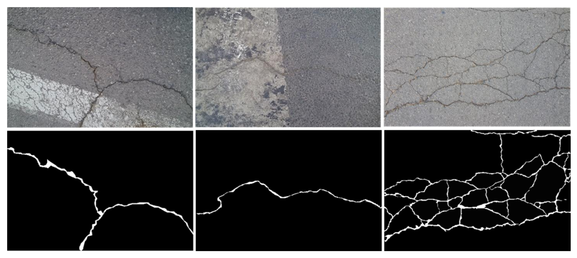
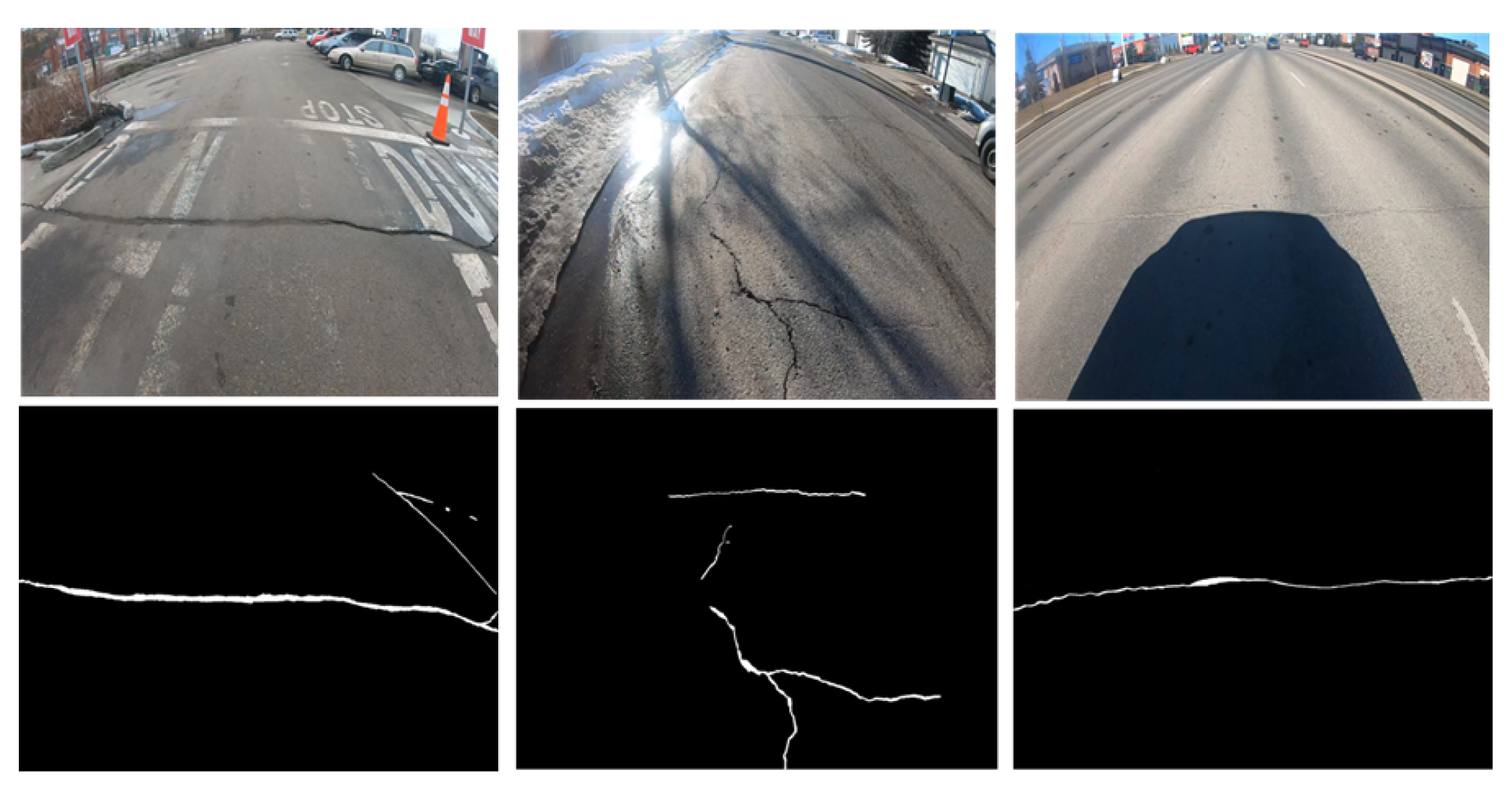
The Edmonton Crack (EdmCrack600) dataset [25] consists of high-resolution images of road cracks, captured with a GoPro Hero 7 Black under diverse environmental conditions, including variations in lighting, weather, and road surface texture. In total, about 3 h videos were taken from different roads in Edmonton, Canada, at different times over two months. Some examples of the dataset are shown in Figure 1. Each image has a resolution of 1920 × 1080 pixels. The dataset includes 600 images with full annotation at the pixel level. These images cover various crack types, such as longitudinal, transverse, and alligator cracks, making EdmCrack600 a comprehensive benchmark for crack detection models [36,37].

Figure 1. Sample of the EdmCrack600 dataset and its annotation.

3.2. CrackForest Dataset

   CrackForest Dataset [26] is an annotated road crack image database that can reflect urban road surface condition in general. It is a widely used benchmark in crack detection research, consisting of 118 images captured from urban roads. These images were taken under relatively uniform lighting conditions and contain diverse types of cracks, including thin and discontinuous patterns. Each image has a resolution of 480 × 320 pixels and is accompanied by manually annotated ground truth masks. Due to its moderate dataset size and well-annotated labels, the CrackForest dataset serves as a valuable test set for assessing the generalization ability of crack segmentation models [38,39]. The cracks in the CrackForest dataset are characteristically thin and elongated. Some examples of the dataset are shown in Figure 2.

Figure 2. Sample of the CrackForest dataset and its annotation.

4. Methodology

   In this section, we provide a detailed explanation of the methodology adopted in this research.

4.1. U-Net++

   U-Net++ [23] is an advanced convolutional neural network (CNN) architecture, originally developed for medical image segmentation and later extended to other domains such as road crack detection [18]. It enhances the classic U-Net [40] by introducing nested and dense skip connections [41], which enable multi-scale feature aggregation and more precise recovery of structural details. The encoder is responsible for capturing contextual information through progressive downsampling, while the decoder reconstructs spatial resolution via upsampling. The key motivation of U-Net++ is to reduce the semantic gap between encoder and decoder feature maps prior to fusion, thereby improving segmentation accuracy, especially for thin or fragmented structures.

In this work, we propose a customized U-Net++ by replacing its standard convolutional encoder with a DenseNet-121 [30] backbone, pretrained on ImageNet. DenseNet-121 is designed to strengthen feature reuse through dense connectivity, where each layer receives inputs from all preceding layers, leading to richer and more discriminative representations. This integration allows the network to capture fine-grained textures of cracks while preserving connectivity, addressing one of the main challenges in road crack segmentation. By leveraging DenseNet’s efficient feature propagation and U-Net++’s nested skip pathways, the proposed model achieves better balance between local detail preservation and global structural consistency, offering a more robust solution for connectivity-aware crack detection.

4.2. SegFormer

   SegFormer [24] is a transformer-based semantic segmentation framework that combines the strengths of both convolutional and transformer architectures. Unlike traditional CNN-based models, SegFormer employs a hierarchical vision transformer encoder known as MiT (Mix Transformer), which captures long-range dependencies and global contextual features through multi-head self-attention mechanisms. The MiT-B5 variant, used in this study, is pre-trained on ImageNet-21k and provides rich multi-scale feature representations while maintaining computational efficiency. SegFormer dispenses with positional encodings and complex decoder designs, instead using a lightweight, multi-layer perceptron (MLP) decoder that aggregates features from different encoder stages. This design enables the model to achieve high accuracy with fewer parameters and faster inference time. Its ability to maintain spatial resolution across scales makes it especially effective for tasks requiring fine structural detail, such as road crack segmentation. Furthermore, the attention-driven feature learning in SegFormer enhances its robustness to varying crack shapes, orientations, and lighting conditions.

4.3. Soft Skeletonization for clDice Loss

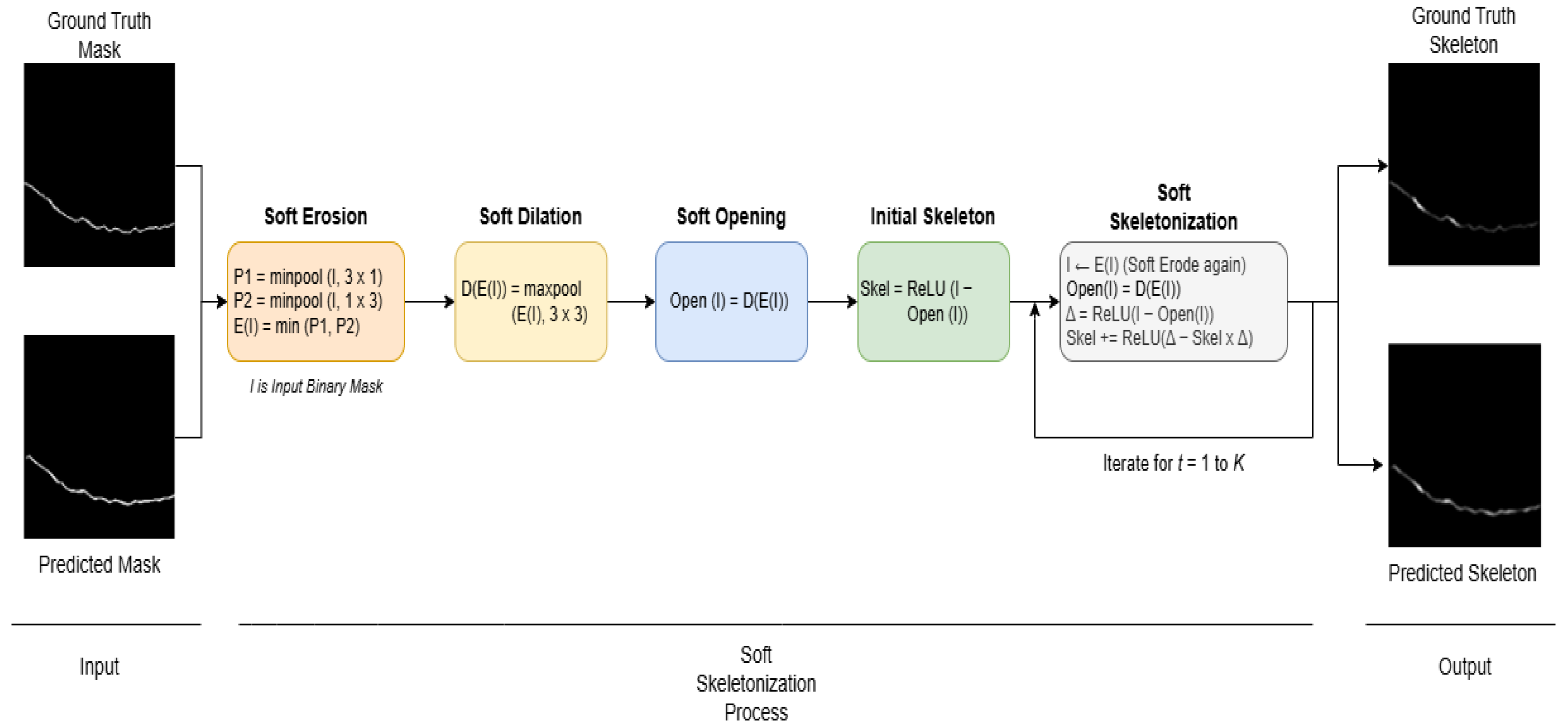
   To incorporate topological priors in the road crack segmentation process, we employ the soft skeletonization algorithm introduced in the clDice loss framework [20]. As illustrated in Figure 3, this algorithm provides a differentiable approximation of morphological skeletonization, allowing backpropagation of gradients through skeleton-like shapes during training. The method is composed of soft versions of erosion, dilation, and skeletonization.

Figure 3. Soft skeletonization process of the road crack mask is integrated with the clDice loss framework. This diagram depicts the step-by-step transformation of both the ground truth mask and the predicted mask into their respective skeletons. The process begins with soft erosion and soft dilation to refine the binary input mask, followed by soft opening to enhance structural clarity. The initial skeleton is derived and further refined through soft skeletonization, incorporating iterative morphological operations over T = 1 to K iterations.

4.3.1. Soft Erosion

The soft erosion operation approximates standard morphological erosion using anisotropic pooling filters in two directions: vertical and horizontal. Then combine them by taking the minimum value. This operation shrinks structures in the image while retaining topological features.

Given an input binary mask image $I\in {[0,1]}^{H\times W}$, we obtain the following:

• Vertical Erosion ($p_1$):

  $$p_1=\mathrm{MinPool}2\mathrm{d}(I;\mathrm{kernel}=3\times 1,\mathrm{padding}=1\times 0)$$

  (1)
• Horizontal Erosion ($p_2$):

  $$p_2=\mathrm{MinPool}2\mathrm{d}(I;\mathrm{kernel}=1\times 3,\mathrm{padding}=0\times 1)$$

  (2)
• Final Output:

  $$\mathrm{soft}\_\mathrm{erode}\left(I\right)=min(p_1,p_2)$$

  (3)

4.3.2. Soft Dilation

The soft dilation operation expands regions in the input eroded image using a standard square max-pooling filter,

$$\mathrm{soft}\_\mathrm{dilate}\left(I\right)=\mathrm{MaxPool}2\mathrm{d}(I;\mathrm{kernel}=3\times 3,\mathrm{padding}=1\times 1)$$

(4)

4.3.3. Soft Opening

The soft opening is a combination of soft erosion followed by soft dilation. It removes small noise while preserving the overall structure,

$$\mathrm{soft}\_\mathrm{open}\left(I\right)=\mathrm{soft}\_\mathrm{dilate}\left(\mathrm{soft}\_\mathrm{erode}\right(I\left)\right)$$

(5)

4.3.4. Soft Skeletonization

The soft skeletonization function iteratively applies soft morphological operations to extract a differentiable skeleton. This skeleton is used to compare the centerlines of segmented objects.

Initialization

Compute the difference between the input and its softly opened version,

$${\mathrm{skel}}_0=\mathrm{ReLU}(I-\mathrm{soft}\_\mathrm{open}\left(I\right))$$

(6)

Iterative Thinning

For each iteration $t\in [1,T]$, where T is the total number of iterations,

$$\begin{array}{cc}\hfill I_t& =\mathrm{soft}\_\mathrm{erode}\left(I_{t-1}\right)\hfill \\ \hfill I_{\mathrm{open}}& =\mathrm{soft}\_\mathrm{open}\left(I_t\right)\hfill \\ \hfill \Delta & =\mathrm{ReLU}(I_t-I_{\mathrm{open}})\hfill \\ \hfill {\mathrm{skel}}_t& ={\mathrm{skel}}_{t-1}+\mathrm{ReLU}(\Delta -{\mathrm{skel}}_{t-1}·\Delta )\hfill \end{array}$$

(7)

Final Output

The soft skeleton at the final iteration is denoted,

$$\mathrm{soft}\_\mathrm{skeleton}(I,T)={\mathrm{skel}}_T$$

(8)

4.3.5. clDice Computation

Once skeletons of the predicted mask P and ground truth mask G are obtained, the clDice score is computed as follows:

Topological Precision

$$T_p={\displaystyle \frac{\left|S\right(P)\cap G|}{\left|S\right(P\left)\right|+ϵ}}$$

(9)

Topological Sensitivity

$$T_g={\displaystyle \frac{\left|S\right(G)\cap P|}{\left|S\right(G\left)\right|+ϵ}}$$

(10)

clDice Score

$$\mathrm{clDice}={\displaystyle \frac{2·T_p·T_g}{T_p+T_g+ϵ}}$$

(11)

4.3.6. clDice Loss

The clDice loss is defined as

$${\mathcal{L}}_{\mathrm{clDice}}=1-\mathrm{clDice}$$

(12)

This loss function encourages both pixel-level and structural correctness, making it particularly suitable for topology-aware segmentation tasks involving thin structures such as road cracks. The complete procedure for computing the soft skeletonization and the subsequent clDice loss is formally summarized in Algorithm 1.

Algorithm 1: Soft Skeletonization and clDice Loss

Input: Predicted mask $P\in {[0,1]}^{H\times W}$, Ground truth mask $G\in {[0,1]}^{H\times W}$, iteration count T, small constant $ϵ$ Output: clDice loss ${\mathcal{L}}_{\mathrm{clDice}}$

Morphological Operators:  1:    $\mathrm{SoftErode}\left(I\right):$    $p_1\leftarrow \mathrm{MinPool}2\mathrm{d}(I,3\times 1,\mathrm{pad}=1\times 0)$    $p_2\leftarrow \mathrm{MinPool}2\mathrm{d}(I,1\times 3,\mathrm{pad}=0\times 1)$    return $min(p_1,p_2)$  2:    $\mathrm{SoftDilate}\left(I\right):$return $\mathrm{MaxPool}2\mathrm{d}(I,3\times 3,\mathrm{pad}=1\times 1)$  3:    $\mathrm{SoftOpen}\left(I\right):$return $\mathrm{SoftDilate}\left(\mathrm{SoftErode}\right(I\left)\right)$ Soft Skeletonization $S\left(I\right)$:  4:    $ske{l}_0\leftarrow \mathrm{ReLU}(I-\mathrm{SoftOpen}\left(I\right))$  5:    $I_0\leftarrow I$  6:    for $t=1$ to T do  7:       $I_t\leftarrow \mathrm{SoftErode}\left(I_{t-1}\right)$  8:       $I_{\mathrm{open}}\leftarrow \mathrm{SoftOpen}\left(I_t\right)$  9:       $\Delta \leftarrow \mathrm{ReLU}(I_t-I_{\mathrm{open}})$  10:       $ske{l}_t\leftarrow ske{l}_{t-1}+\mathrm{ReLU}(\Delta -ske{l}_{t-1}·\Delta )$  11:    end for  12:    return $S\left(I\right)\leftarrow ske{l}_T$ clDice Computation:  13:    $S\left(P\right)\leftarrow \mathrm{SoftSkeleton}(P,T)$  14:    $S\left(G\right)\leftarrow \mathrm{SoftSkeleton}(G,T)$  15:    $T_p\leftarrow {\displaystyle \frac{\left|S\right(P)\cap G|}{\left|S\right(P\left)\right|+ϵ}}$  16:    $T_g\leftarrow {\displaystyle \frac{\left|S\right(G)\cap P|}{\left|S\right(G\left)\right|+ϵ}}$  17:    $\mathrm{clDice}\leftarrow {\displaystyle \frac{2·T_p·T_g}{T_p+T_g+ϵ}}$  18:    ${\mathcal{L}}_{\mathrm{clDice}}\leftarrow 1-\mathrm{clDice}$  19:    return ${\mathcal{L}}_{\mathrm{clDice}}$

5. Experimental Setup

5.1. Determination of Optimal Skeletonization Iterations

Before training the segmentation model, we performed an offline analysis to determine the appropriate number of iterations k for the soft skeletonization process. Since the number of iterations affects the thickness and extent of the extracted skeleton, we visually evaluated the skeletonization results over a range of $k\in \{5,10,15,20,25,30,35\}$ on a representative subset of the training data. This analysis was performed using the CPU and did not involve model training. The goal was to identify a value of k that produces clean, thin, and topologically representative skeletons for crack-like structures.

Figure 4 illustrates the evolution of the soft skeletonization process applied to a sample crack mask across seven different iteration values. As k increases, the skeletons become progressively cleaner and more refined, revealing a gradual improvement in connectivity while reducing background noise. After k = 30, there is no further change in the skeleton result, indicating convergence of the process. Based on these visual observations, we proceeded to conduct quantitative experiments across all k values to systematically evaluate their impact on segmentation performance and verify whether the qualitative improvements lead to measurable gains in segmentation metrics. The quantitative results will ultimately determine the optimal fixed k value that will be used for comparative experiments against other baseline loss functions.

Figure 4. Visual progression of the soft skeletonization process applied to a road crack mask at seven different iteration counts: $k=5,10,15,20,25,30$ and 35. As k increases, the skeleton becomes progressively cleaner and more refined, improving continuity and reducing noise.

5.2. Training Methodology

We utilize two advanced architectures for semantic segmentation: U-Net++ [23] and SegFormer [24]. For our U-Net++ implementation, we enhance the encoder by integrating a DenseNet-121 backbone [30] pre-trained on ImageNet. This modification introduces dense connectivity patterns that improve gradient flow and feature reuse across network layers, thereby helping the model learn more complex patterns. For SegFormer, we adopt the MiT-B5 backbone, which is pre-trained on ImageNet-21k, enabling robust semantic feature extraction through its lightweight, attention-based transformer modules. To ensure robust performance evaluation, we employ 5-fold cross-validation. The dataset is randomly partitioned into five equal subsets. In each fold, 70% of the data is used for training, 20% for validation, and the remaining 10% for testing. This ensures that every sample appears in the test set exactly once over the five folds. To mitigate overfitting and increase data diversity, we apply several augmentation techniques during training, including horizontal flipping (50% probability), random rotations within $\pm {15}^{\circ }$, and gamma correction to simulate varying lighting conditions, following the strategy described in [42]. All images are resized to $256\times 256$ pixels prior to training to ensure uniform input dimensions. Model optimization is performed using the AdamW optimizer [43]. We conduct a grid search over key hyperparameters, exploring learning rates $\left\{1\times {10}^{-4},5\times {10}^{-4},1\times {10}^{-3}\right\}$, weight decay values $\left\{1\times {10}^{-4},1\times {10}^{-3},1\times {10}^{-2}\right\}$, and batch sizes $\left\{8,16,32\right\}$. The best configuration learning rate of $1\times {10}^{-4}$, weight decay of $1\times {10}^{-3}$, and batch size of 8 is used to train the final models for 100 epochs. All experiments are implemented in Python 3.12.7 using PyTorch 2.2.0. The training and evaluation are conducted on a workstation equipped with an Intel i5-12600K CPU, 64 GB RAM, and an NVIDIA RTX A6000 GPU. This experimental setup is consistently applied across both the EdmCrack600 [25] and CrackForest [26] datasets.

5.3. Loss Function

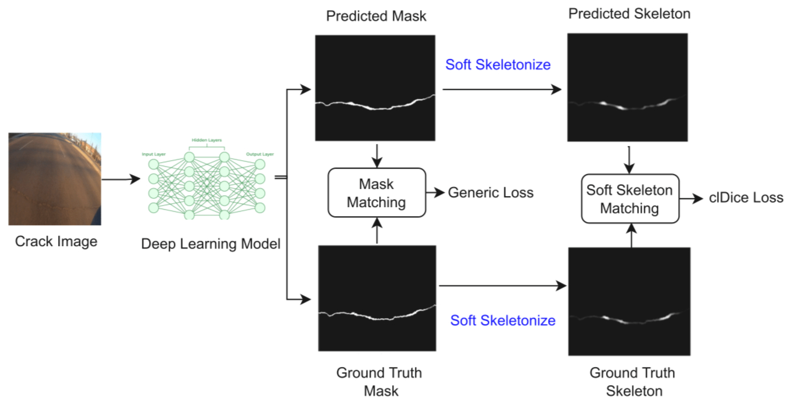
Since the clDice loss uses skeletal properties to ensure correct topology, not just to learn skeletons, it is insufficient as a standalone loss function for achieving both topological correctness and overall segmentation accuracy [20]. In this study, our objective is not only to achieve the skeleton as the primary output but also to produce segmentations that are both topologically accurate and precise. The model is trained using a combination of the clDice and other generic losses. The clDice loss is employed to enhance the ability of the model to capture topological features, such as the structure of segmented regions, which is particularly critical for road crack detection tasks. Conversely, the generic losses focus on maximizing the overlap between the predicted segmentation and the ground truth. Figure 5 illustrates the combined process of both clDice and generic loss. The total loss is formulated as a weighted sum of the clDice loss and a generic segmentation loss, as shown in Equation (13) below:

$$L_{\mathrm{total}}=(\lambda ·L_{\mathrm{clDice}})+\left(L_{\mathrm{Generic}\mathrm{Loss}}\right)$$

(13)

Figure 5. Combination of clDice and generic loss functions in a deep learning model. This diagram illustrates the process where a crack image is processed through a deep learning model to generate a predicted mask and a predicted skeleton. The predicted mask undergoes mask matching with the ground truth mask, utilizing a generic loss function to evaluate the similarity, while the predicted skeleton is compared with the ground truth skeleton using clDice loss through soft skeleton matching.

Here, $L_{\mathrm{clDice}}$ denotes the clDice loss, $L_{\mathrm{generic}}$ represents the baseline segmentation loss (e.g., Dice, BCE, or IoU), and the scalar hyperparameter $\lambda$ controls the influence of the clDice term. Adjusting $\lambda$ allows us to trade off topological accuracy (captured by clDice) against regional overlap (captured by the generic loss). To determine an optimal balance, we systematically tried a range of $\lambda$ from 0.1 to 0.9 (Appendix A). This evaluation helped find the value of $\lambda$ that balances preserving the correct crack structure and achieving accurate pixel-level prediction.

5.4. Evaluation Metrics

To evaluate the performance of the proposed segmentation models, we employ several metrics that assess both region overlap and topological accuracy. These metrics include Dice coefficient [18], Intersection over Union (IoU) [27], Center Line Dice (clDice) [20], and Hausdorff Distance [28]. They offer a comprehensive metric of both the pixel-wise and structural quality of the segmentation.

5.4.1. Dice Coefficient

The Dice coefficient [18], also known as the F1 score in binary segmentation, measures the overlap between the predicted mask P and the ground truth G. It is defined as

$$\mathrm{Dice}(G,P)={\displaystyle \frac{2|G\cap P|}{\left|G\right|+\left|P\right|}}$$

(14)

This metric ranges from 0 (no overlap) to 1 (perfect overlap), and is particularly useful in class-imbalanced segmentation tasks.

5.4.2. Intersection over Union (IoU)

Also known as the Jaccard Index [27], the IoU quantifies the percentage overlap between the ground truth and the predicted segmentation,

$$\mathrm{IoU}(G,P)={\displaystyle \frac{|G\cap P|}{|G\cup P|}}$$

(15)

IoU penalizes both false positives and false negatives and is widely used in semantic segmentation benchmarks.

5.4.3. Center Line Dice (clDice)

The clDice metric [20] is designed to evaluate the topological accuracy of thin and tubular structures by comparing the skeletons of the prediction and ground truth. It combines two asymmetric soft Dice scores: one between the prediction and the skeleton of the ground truth, and the other between the ground truth and the skeleton of the prediction,

$$\mathrm{clDice}(G,P)={\displaystyle \frac{2·T(G,P)·T(P,G)}{T(G,P)+T(P,G)}}$$

(16)

where

$$T(G,P)={\displaystyle \frac{\left|S\right(G)\cap P|}{\left|S\right(G\left)\right|}},T(P,G)={\displaystyle \frac{\left|S\right(P)\cap G|}{\left|S\right(P\left)\right|}}$$

(17)

and $S(·)$ denotes the soft skeletonization function. clDice captures how well the predicted structure aligns with the centerline of the ground truth, making it ideal for crack detection tasks.

5.4.4. Hausdorff Distance

Hausdorff Distance (HD) [28] measures the greatest of all the distances from a point in one set to the closest point in the other set. For predicted mask P and ground truth G, it is defined as

$$\mathrm{HD}(G,P)=max\left\{\underset{g\in G}{sup}\underset{p\in P}{inf}d(g,p),\underset{p\in P}{sup}\underset{g\in G}{inf}d(p,g)\right\}$$

(18)

where $d(·,·)$ is the Euclidean distance. This metric evaluates the worst-case boundary discrepancy, useful for assessing structural alignment.

6. Experimental Result

6.1. Quantitative Validation of Skeletonization Iterations

To validate the qualitative observations from Section 5.1 and determine the optimal iteration count empirically, we conducted comprehensive quantitative experiments across all k values.

6.1.1. SegFormer with clDice-Based Losses

The results for the SegFormer model are shown in Table 1, Table 2, Table 3 and Table 4. The results show a clear positive response as k increases. They also confirm that the visual improvements observed during skeleton refinement directly correlate with measurable gains in segmentation performance across all evaluated metrics.

Table 1. Quantitative results of SegFormer on the EdmCrack600 dataset using clDice + Dice loss with different skeletonization iterations k.

k	Metric
	Dice	IoU	clDice	Hasd. Dist.
5	0.737	0.597	0.772	36.369
10	0.745	0.608	0.778	34.000
15	0.753	0.618	0.785	30.500
20	0.762	0.630	0.792	27.000
25	0.768	0.638	0.796	24.000
30	0.771	0.641	0.798	23.310
35	0.769	0.643	0.796	23.355

Table 2. Quantitative results of SegFormer on the EdmCrack600 dataset using clDice + IoU loss with different skeletonization iterations k.

k	Metric
	Dice	IoU	clDice	Hasd. Dist.
5	0.735	0.596	0.781	36.160
10	0.740	0.603	0.783	34.000
15	0.746	0.611	0.787	30.000
20	0.752	0.619	0.791	26.500
25	0.758	0.627	0.794	24.000
30	0.761	0.626	0.794	22.061
35	0.760	0.627	0.793	22.500

Table 3. Quantitative results of SegFormer on the CrackForest dataset using clDice + Dice loss with different skeletonization iterations k.

k	Metric
	Dice	IoU	clDice	Hasd. Dist.
5	0.830	0.714	0.901	15.051
10	0.840	0.729	0.907	15.393
15	0.852	0.745	0.918	12.000
20	0.861	0.758	0.926	9.000
25	0.870	0.772	0.932	6.500
30	0.874	0.780	0.936	4.303
35	0.873	0.781	0.933	5.040

Table 4. Quantitative results of SegFormer on the CrackForest dataset using clDice + IoU loss with different skeletonization iterations k.

k	Metric
	Dice	IoU	clDice	Hasd. Dist.
5	0.841	0.731	0.909	11.917
10	0.844	0.736	0.913	10.500
15	0.849	0.743	0.917	9.000
20	0.854	0.750	0.920	7.500
25	0.859	0.757	0.923	6.500
30	0.862	0.761	0.925	5.803
35	0.860	0.758	0.923	5.800

The performance across all metrics consistently improved as k increased from 5 to 30 on both datasets. This demonstrates that transformer-based architectures also benefit significantly from the refined topological guidance provided by higher iteration skeletons. The performance reaches its optimum at $k=30$, with $k=35$ showing only marginal differences, suggesting convergence of the skeletonization process for this model.

6.1.2. U-Net++ with clDice-Based Losses

As shown in Table 5, Table 6, Table 7 and Table 8, the results for U-Net++ demonstrate an even more pronounced and consistent trend as k increases from 5 to 30 across both datasets. These results highlight the strong synergy between convolutional inductive biases and topological constraints.

Table 5. Quantitative results of U-Net++ on the EdmCrack600 dataset using clDice + Dice loss with different skeletonization iterations k.

k	Metric
	Dice	IoU	clDice	Hasd. Dist.
5	0.775	0.642	0.814	32.710
10	0.781	0.648	0.821	31.940
15	0.788	0.655	0.829	31.910
20	0.797	0.665	0.837	30.523
25	0.810	0.697	0.844	29.900
30	0.824	0.709	0.850	29.280
35	0.823	0.709	0.849	29.281

Table 6. Quantitative results of U-Net++ on the EdmCrack600 dataset using clDice + IoU loss with different skeletonization iterations k.

k	Metric
	Dice	IoU	clDice	Hasd. Dist.
5	0.795	0.669	0.829	30.764
10	0.805	0.681	0.838	30.108
15	0.815	0.693	0.845	29.610
20	0.822	0.702	0.849	29.224
25	0.828	0.715	0.851	28.576
30	0.830	0.720	0.852	28.263
35	0.831	0.712	0.850	28.267

Table 7. Quantitative results of U-Net++ on the CrackForest dataset using clDice + Dice loss with different skeletonization iterations k.

k	Metric
	Dice	IoU	clDice	Hasd. Dist.
5	0.904	0.829	0.941	10.908
10	0.910	0.837	0.951	9.502
15	0.915	0.845	0.957	9.588
20	0.918	0.850	0.960	8.600
25	0.920	0.853	0.962	8.375
30	0.921	0.855	0.964	8.222
35	0.921	0.856	0.961	8.300

Table 8. Quantitative results of U-Net++ on the CrackForest dataset using clDice + IoU loss with different skeletonization iterations k.

k	Metric
	Dice	IoU	clDice	Hasd. Dist.
5	0.837	0.727	0.898	29.336
10	0.864	0.771	0.911	17.083
15	0.885	0.800	0.945	11.001
20	0.902	0.825	0.949	9.000
25	0.915	0.845	0.952	8.000
30	0.923	0.859	0.957	7.531
35	0.919	0.851	0.958	7.686

The U-Net++ model showed robust performance gains as k increased, peaking at $k=30$. The architecture’s inherent strength in local feature extraction appears to be effectively guided by the topological prior from the clDice loss, leading to superior overall results. The optimal performance was consistently achieved at $k=30$, reinforcing its suitability.

Overall Analysis and Selection of k

The results from both Section 6.1.1 and Section 6.1.2 lead to a consistent conclusion. At lower iterations (k = 5–15), the skeletonization process produces less refined skeletons that retain excessive background noise and fail to capture the precise topological structure of thin cracks. This results in suboptimal segmentation performance for both SegFormer and U-Net++. As k increases to 20–25, the skeletons progressively become cleaner and more representative of true crack connectivity. This leads to consistent improvements in all metrics. Optimal performance is achieved between $k=30$ and $k=35$ for both architectures, indicating that the skeletonization process has converged and that further iterations provide diminishing returns. While $k=35$ achieved marginally better scores in certain configurations, $k=30$ demonstrates superior and more consistent performance across the vast majority of experimental configurations and both model architectures. It achieves the optimal balance between skeleton quality and segmentation accuracy. Based on this comprehensive quantitative validation, we selected $k=30$ as the fixed iteration count for all subsequent comparative experiments against baseline loss functions.

6.2. Comparison Experiment Results

Building upon the validated optimal iteration count of $k=30$ from Section 6.1, we conducted comprehensive comparison experiments between clDice-based losses and other baseline loss functions. The performance of SegFormer and customized U-Net++ models on the EdmCrack600 and CrackForest datasets was evaluated using various loss functions to investigate the effectiveness of the clDice loss for road crack segmentation, with the models used only to evaluate the performance of the loss functions, not to compare the models themselves. The analysis focused on connectivity accuracy (clDice and Hausdorff Distance) and overall accuracy (Dice and IoU) to compare the performance of different loss functions against clDice-based losses. The optimal weight parameter values for each dataset were chosen based on configuration experiments exploring different lambda values (results provided in Appendix A).

6.2.1. Comparison Result on EdmCrack600 Dataset

Based on the quantitative result in Table 9 for the EdmCrack600 dataset, using a skeletonization value $k=30$ and loss weight $\lambda =0.5$, the “clDice + Dice” configuration with SegFormer achieved the highest Dice (0.771), IoU (0.641), and clDice (0.798), with a Hausdorff Distance of 23.310. Meanwhile, the “clDice + IoU” yielded a Hausdorff Distance of 22.061. Interestingly, the BCE loss achieved a higher Hausdorff Distance (38.665) and a lower clDice (0.651), indicating that clDice-based losses performed better in both connectivity and precise placement. The clDice-based combinations clearly outperformed BCE and other combined conventional losses in terms of clDice, Dice, and IoU scores, indicating stronger structural and region based accuracy.

Table 9. Performance evaluation of loss functions on the EdmCrack600 dataset using SegFormer and customized U-Net++ models.

Model	Loss Function	Metric				Computational Time
		Dice	IoU	clDice	Hasd. Dist.	Training (Minutes)	Inference (Seconds)
SegFormer	BCE	0.660	0.520	0.651	38.665	20.491	1.134
	Dice	0.720	0.583	0.755	37.669	20.431	1.098
	IoU	0.738	0.599	0.773	35.853	20.444	1.146
	Dice + BCE	0.737	0.597	0.773	34.246	20.385	1.107
	IoU + BCE	0.739	0.600	0.782	26.744	20.603	1.098
	clDice + Dice	0.771	0.641	0.798	23.310	20.368	1.112
	clDice + IoU	0.761	0.626	0.794	22.061	20.293	1.183
U-Net++	BCE	0.781	0.650	0.813	40.577	20.233	0.389
	Dice	0.811	0.691	0.838	34.417	20.260	0.392
	IoU	0.803	0.682	0.836	29.435	20.259	0.422
	Dice + BCE	0.819	0.701	0.853	30.226	20.180	0.393
	IoU + BCE	0.813	0.693	0.842	31.429	20.171	0.399
	clDice + Dice	0.824	0.709	0.850	29.280	20.017	0.409
	clDice + IoU	0.830	0.720	0.852	28.263	20.233	0.401

Similarly, for customized U-Net++, “clDice + IoU” recorded the highest Dice (0.830), IoU (0.720), and clDice (0.852), with a Hausdorff Distance of 28.263. The “clDice + Dice” configuration yielded a Hausdorff Distance of 29.280. The clDice-based losses consistently achieved higher clDice and overlap metrics than traditional losses such as BCE (clDice 0.813, Hausdorff 40.577) and Dice (clDice 0.838, Hausdorff 34.417). This underscores the effectiveness of clDice loss in improving road crack segmentation, especially in preserving the shape and continuity of the cracks.

6.2.2. Comparison Result on CrackForest Dataset

The effectiveness of the clDice loss for road crack segmentation was further examined on the CrackForest dataset using a loss weight $\lambda =0.4$. The result in Table 10 shows that for SegFormer, the “clDice + Dice” configuration demonstrated superior performance with the highest clDice (0.936), Dice (0.874), and IoU (0.780), paired with the lowest Hausdorff distance (4.303). This outperformed single losses like BCE (clDice 0.873, Hausdorff 13.187) and Dice (clDice 0.900, Hausdorff 12.640) in terms of connectivity and segmentation quality. Consistently, customized U-Net++ highlighted the superiority of the clDice-based configurations. The “clDice + IoU” loss achieved the highest Dice (0.923) and IoU (0.859), while the “clDice + Dice” configuration yielded the highest clDice (0.964). Both clDice combinations achieved lower Hausdorff distances, with “clDice + IoU” at 7.531, surpassing BCE (clDice 0.940, Hausdorff 9.073) and Dice (clDice 0.941, Hausdorff 8.414). These findings reinforce that clDice-based loss functions significantly boost connectivity and overall accuracy, validating their effectiveness for improved road crack segmentation on the CrackForest dataset.

Table 10. Performance evaluation of loss functions on CrackForest dataset using SegFormer and customized U-Net++ models.

Model	Loss Function	Metric				Computational Time
		Dice	IoU	clDice	Hasd. Dist.	Training (Minutes)	Inference (Seconds)
SegFormer	BCE	0.811	0.689	0.873	13.187	3.118	0.224
	Dice	0.841	0.732	0.900	12.640	3.099	0.222
	IoU	0.842	0.735	0.900	11.887	3.101	0.221
	Dice + BCE	0.843	0.733	0.905	11.650	3.083	0.222
	IoU + BCE	0.844	0.736	0.910	5.769	3.092	0.221
	clDice + Dice	0.874	0.780	0.936	4.303	3.228	0.225
	clDice + IoU	0.862	0.761	0.925	5.803	3.181	0.221
U-Net++	BCE	0.895	0.817	0.940	9.073	2.714	0.088
	Dice	0.900	0.821	0.941	8.414	2.786	0.078
	IoU	0.891	0.806	0.936	10.268	2.738	0.078
	Dice + BCE	0.912	0.843	0.942	10.868	2.724	0.079
	IoU + BCE	0.907	0.823	0.948	7.713	2.715	0.087
	clDice + Dice	0.921	0.855	0.964	8.222	1.352	0.098
	clDice + IoU	0.923	0.859	0.957	7.531	2.847	0.080

7. Discussion and Future Task

The experimental results from the EdmCrack600 and CrackForest datasets provide valuable insights into the effectiveness of the clDice loss function for road crack segmentation. The analysis focused on three key aspects: connectivity (the structural completeness of cracks, measured by clDice), boundary precision (the precise placement of predictions, measured by Hausdorff Distance), and computational efficiency (training and inference time). Additionally, we evaluated overall segmentation performance using standard overlap metrics (Dice and IoU). Across both datasets, loss combinations incorporating clDice, especially when balanced with Dice or IoU using a weight $\lambda =0.4$ and $\lambda =0.5$, and a skeletonization iteration $k=30$, consistently outperformed traditional single loss functions in enhancing segmentation quality.

The sensitivity analysis of the clDice weight $\lambda$ (see Appendix A) reveals a clear pattern: performance peaks at a balanced value (typically $\lambda =0.4$ or $0.5$) and then gradually declines. This indicates that an optimal trade-off exists where clDice effectively guides topology preservation without overwhelming the region-based loss. Notably, at higher $\lambda$ values (e.g., 0.8, 0.9), we observe a consistent performance drop across most metrics. This suggests the model may over-prioritize connectivity at the expense of precise localization rather than overfitting to the training data.

The computational complexity analysis in Table 9 and Table 10 reveals important practical considerations for clDice deployment. The iterative soft skeletonization process in clDice, with complexity proportional to the number of iterations k, introduces additional overhead compared to traditional losses. However, our timing results show that clDice-based losses achieved competitive training times, in some cases even faster than baseline methods (e.g., clDice + Dice with U-Net++ on CrackForest trained in 1.35 min compared to 2.71 min for BCE). While inference times remain comparable across all loss functions, the training efficiency makes clDice practically deployable despite its additional computational requirements.

The practical deployment of clDice also depends on the underlying model architecture. Our results show a clear performance trend, with the customized U-Net++ model achieving superior results across all metrics (Dice, IoU, clDice, and Hausdorff Distance) on both datasets compared to SegFormer. This performance gap is likely due to the fundamental differences in their design and capacity. To ensure a fair comparison, we note that our customized U-Net++ has approximately 9.0 million parameters, while the SegFormer model (MIT-B5 backbone) used has over 80 million parameters. This indicates that the performance difference is not due to a disparity in model capacity. Furthermore, as shown in Table 9 and Table 10, U-Net++ demonstrated significantly faster inference times (e.g., 0.4 s vs. 1.1 s on EdmCrack600), highlighting its computational efficiency. Additionally, Transformer-based models like SegFormer are typically data-hungry and often require larger datasets to fully leverage their ability to model long-range dependencies. In contrast, the convolutional inductive biases of U-Net++, such as its hierarchical feature extraction and precise localization capabilities, make it particularly well-suited for the task of segmenting thin, elongated crack structures, even with the available dataset sizes. Therefore, the superior performance and efficiency of U-Net++ are more strongly attributed to its architectural inductive biases than to its parameter count.

These clDice-based combinations demonstrated superior preservation of thin, elongated crack structures, as indicated by improved clDice scores. While they generally also improved boundary precision (Hausdorff Distance), the traditional BCE loss occasionally achieved a marginally better score on this specific metric in isolated cases (e.g., on EdmCrack600 with SegFormer). This phenomenon can be explained by describing the different objectives of the losses. The BCE loss penalizes all pixel-level errors equally. This can lead to conservative, high-precision predictions that avoid isolated false positive pixels far from the ground truth. This is why it yielded a lower result for Hausdorff Distance. In contrast, the clDice loss actively encourages predicting long, connected structures that match the topology of the skeleton. This can result in the model extending a crack prediction slightly beyond its true endpoint to maintain connectivity, which the Hausdorff metric penalizes more heavily. Therefore, BCE may occasionally yield a superior Hausdorff distance by failing to capture the full extent of the crack. Conversely, clDice prioritizes structural completeness, which may result in minor losses in extreme boundary accuracy. This suggests that clDice effectively ensures continuous predictions but at the slight cost of boundary precision.

This work improves the reliability of automated crack inspections by addressing the fundamental challenge of accurately segmenting connected crack topologies. In pavement assessment and structural health monitoring, distinguishing a single, continuous, propagating crack is crucial because it has significant implications for structural integrity. The proposed skeleton-based loss function ensures automated systems preserve connectivity, producing segmentation maps that accurately represent the crack network. These reliable topological representations provide engineers with the necessary data to make informed decisions about maintenance prioritization.

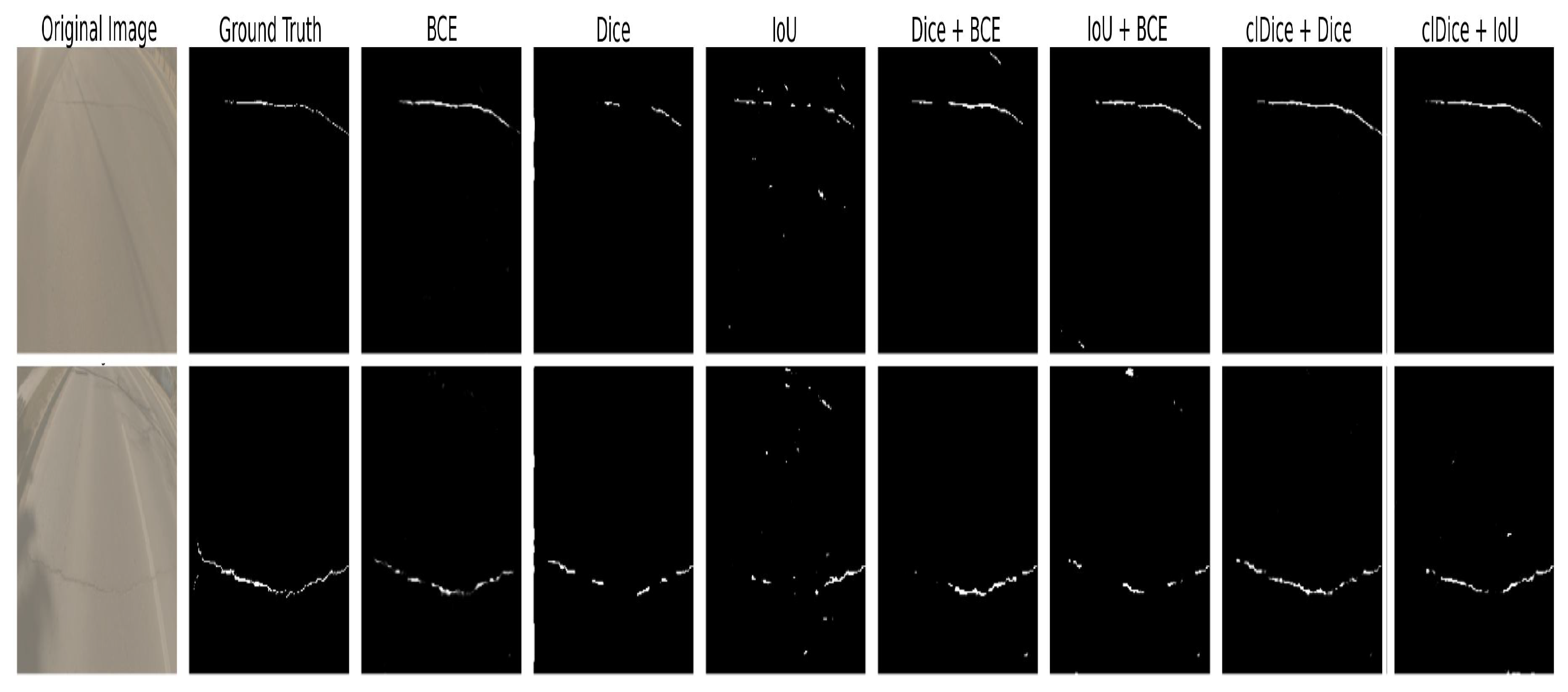
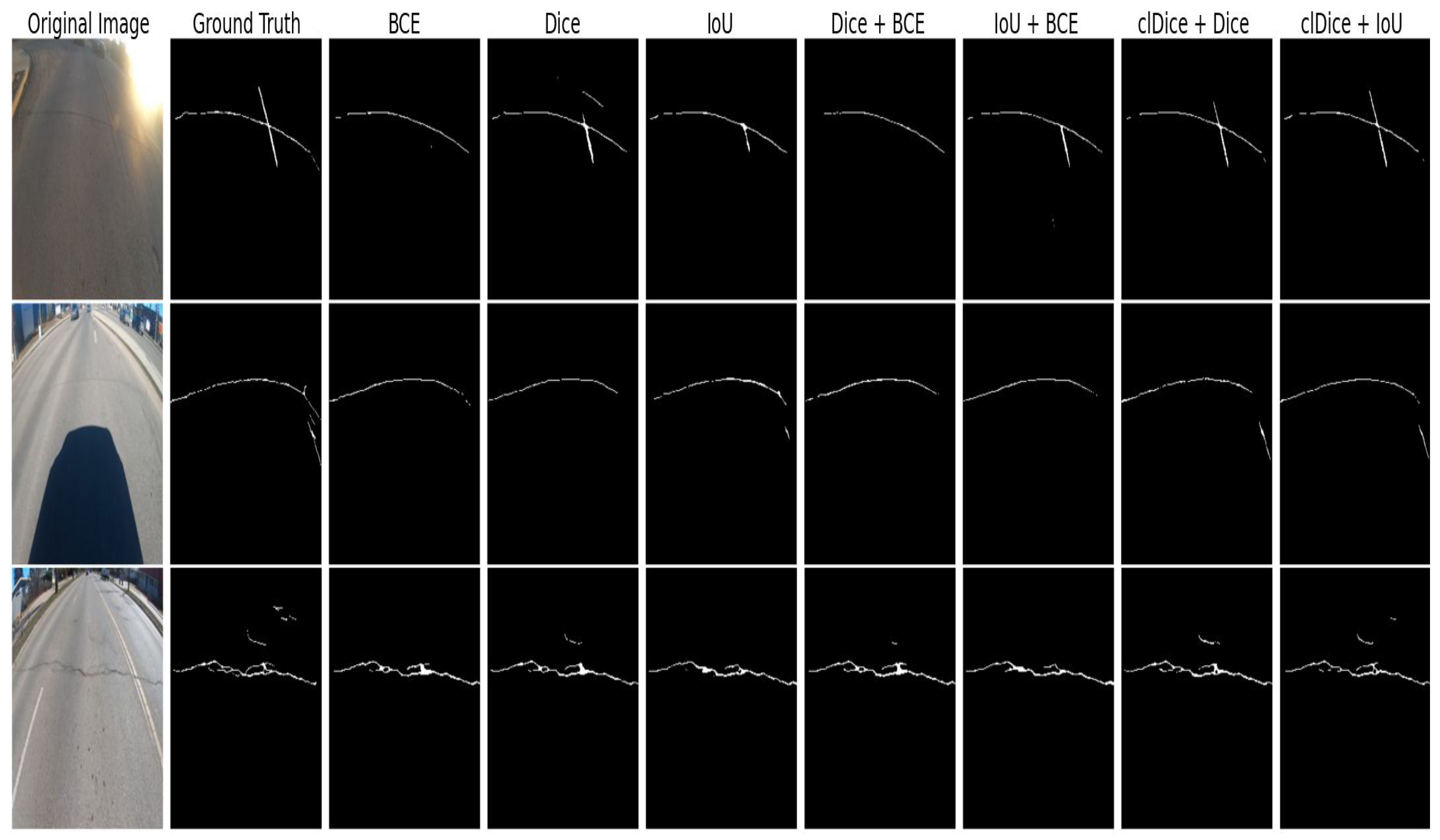
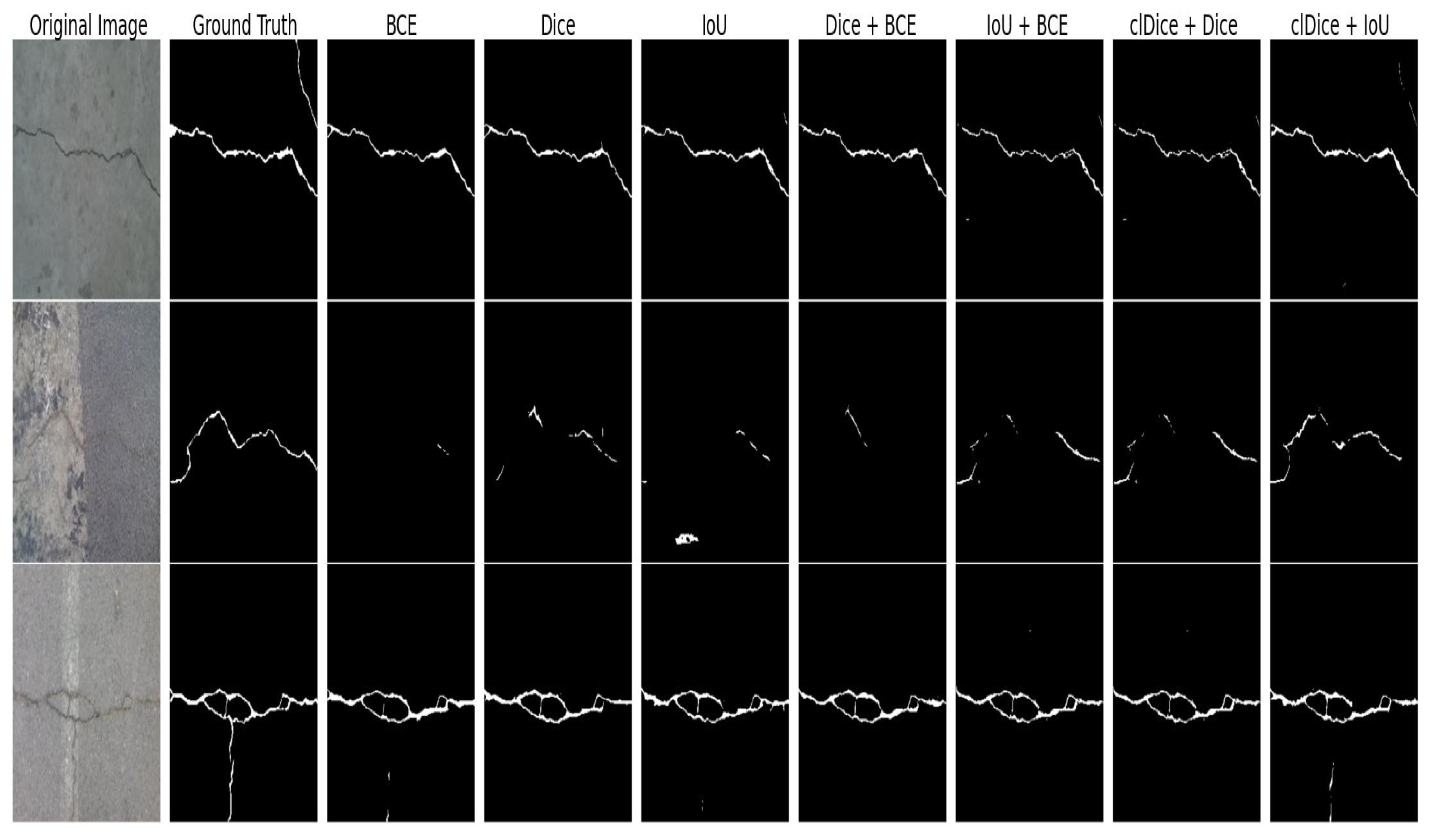
Conventional losses often resulted in fragmented segmentations or over-segmentation in challenging regions, such as under strong illumination or where crack structures are vertically aligned. In Figure 6, IoU loss produces the worst prediction, except BCE loss almost successfully detects the crack areas in both images compared to other baseline losses. In contrast, clDice + Dice and clDice + IoU provide more continuous and complete predictions, even though clDice + IoU produces a small oversegmented part. Similar result shown in Figure 7, in the third row, Dice and IoU + BCE fail to capture all the crack lines, while IoU slightly over-segments the regions. In contrast, clDice-based losses (clDice + Dice and clDice + IoU) consistently produce more continuous and complete crack predictions, effectively preserving connectivity and structural accuracy in challenging areas. In Figure 8 on the CrackForest dataset, the baseline losses such as BCE, IoU, and Dice + BCE struggle to detect most of the horizontal cracks and often miss small vertical lines. In contrast, clDice-based losses (clDice + Dice and clDice + IoU) produce more continuous and accurate crack predictions, with clDice + IoU excelling in preserving connectivity and structural accuracy.

Figure 6. Qualitative results on the EdmCrack600 dataset using the SegFormer model with different loss functions. BCE loss almost successfully detects the crack areas in both images compared to other baseline losses. In contrast, clDice + Dice and clDice + IoU provide more continuous and complete predictions, even though clDice + IoU produces a small oversegmented part.

Figure 7. Qualitative results using customized U-Net++ model trained with different loss functions on the EdmCrack600 dataset. In the first row, BCE and Dice+BCE fail to capture the vertical crack line, while Dice slightly over-segments the region under strong illumination. In the second and third rows, almost all baseline losses miss the small vertical and horizontal crack entirely. In contrast, clDice-based losses (clDice + Dice and clDice + IoU) consistently produce more continuous and complete crack predictions, effectively preserving connectivity and structural accuracy in challenging areas.

Figure 8. Qualitative results on the CrackForest dataset using a customized U-Net++ model with different loss functions. In the second row, BCE, Dice, and Dice + BCE struggle to detect most of the crack areas, with IoU showing slight over-segmentation. In contrast, clDice + Dice and clDice + IoU provide more continuous and complete predictions, with clDice + IoU producing better results in preserving crack connectivity and structural accuracy.

Overall, integrating clDice with region-based losses not only improves topological accuracy (connectivity) but also enhances general segmentation performance across both convolution-based (U-Net++) and transformer-based (SegFormer) models. The findings underscore the robustness and adaptability of clDice-based loss configurations, making them well-suited for road crack segmentation tasks involving thin and complex structural shapes.

A future task could extend this work by comparing the performance of clDice with other advanced topological loss functions to explore further the trade-offs between connectivity preservation and boundary precision for highly fragmented crack networks.

8. Conclusions

This study explored the effectiveness of the clDice loss function for road crack segmentation, with a focus on its enhancement when integrated with Dice or IoU losses. Experiments were performed using customized U-Net++, and SegFormer models across two distinct datasets, EdmCrack600 and CrackForest, which exhibit varied crack patterns. The findings consistently indicate that a balanced combination of clDice with Dice or IoU loss, using a weight $\lambda =0.4$ and $\lambda =0.5$, and skeletonization iteration $k=30$, delivers optimal performance, effectively capturing thin, elongated cracks by preserving their centerline and structural consistency. This setup achieved the highest Dice scores, ensuring precise segmentation of crack regions. However, an overemphasis on clDice resulted in reduced Dice scores, suggesting that excessive weighting may compromise region overlap accuracy, while underweighting clDice still yielded respectable Dice performance, though the balanced approach proved most effective.

The results underscore that clDice-based combinations enhance segmentation quality, particularly for fine structural details, with both customized U-Net++ and SegFormer benefiting from this strategy. The computational efficiency analysis demonstrates that clDice-based losses achieve competitive training times despite the additional skeletonization overhead, making them suitable for practical deployment in automated inspection systems. These findings have significant implications for automated pavement inspection and structural health monitoring, where accurate crack connectivity assessment is crucial for maintenance prioritization and safety evaluation. This approach offers a practical advancement for automated road monitoring systems and provides a foundation for improving segmentation of linear structures in infrastructure assessment and related fields.

References

1. Ng, C.P.; Law, T.H.; Jakarni, F.M.; Kulanthayan, S. Road infrastructure development and economic growth. IOP Conf. Ser. Mater. Sci. Eng. 2019, 512, 012045. [Google Scholar] [CrossRef]
2. Mohan, A.; Poobal, S. Crack detection using image processing: A critical review and analysis. Alex. Eng. J. 2018, 57, 787–798. [Google Scholar] [CrossRef]
3. Feng, X.; Xiao, L.; Li, W.; Pei, L.; Sun, Z.; Ma, Z.; Shen, H.; Ju, H. Pavement Crack Detection and Segmentation Method Based on Improved Deep Learning Fusion Model. Math. Probl. Eng. 2020, 2020, 1–22. [Google Scholar] [CrossRef]
4. Nguyen, S.D.; Tran, T.S.; Tran, V.P.; Lee, H.J.; Piran, M.J.; Le, V.P. Deep Learning-Based Crack Detection: A Survey. Int. J. Pavement Res. Technol. 2023, 16, 943–967. [Google Scholar] [CrossRef]
5. Liu, Y.; Yao, J.; Lu, X.; Xie, R.; Li, L. DeepCrack: A deep hierarchical feature learning architecture for crack segmentation. Neurocomputing 2019, 338, 139–153. [Google Scholar] [CrossRef]
6. Cha, Y.J.; Choi, W.; Büyüköztürk, O. Deep Learning-Based Crack Damage Detection Using Convolutional Neural Networks. Comput.-Aided Civ. Infrastruct. Eng. 2017, 32, 361–378. [Google Scholar] [CrossRef]
7. Ran, R.; Xu, X.; Qiu, S.; Cui, X.; Wu, F. Crack-SegNet: Surface Crack Detection in Complex Background Using Encoder-Decoder Architecture. In ACM International Conference Proceeding Series; Association for Computing Machinery: New York, NY, USA, 2021. [Google Scholar] [CrossRef]
8. Di Benedetto, A.; Fiani, M.; Gujski, L.M. U-Net-Based CNN Architecture for Road Crack Segmentation. Infrastructures 2023, 8, 90. [Google Scholar] [CrossRef]
9. Liu, H.; Yang, J.; Miao, X.; Mertz, C.; Kong, H. CrackFormer Network for Pavement Crack Segmentation. IEEE Trans. Intell. Transp. Syst. 2023, 24, 9240–9252. [Google Scholar] [CrossRef]
10. Guo, F.; Liu, J.; Lv, C.; Yu, H. A novel transformer-based network with attention mechanism for automatic pavement crack detection. Constr. Build. Mater. 2023, 391, 131852. [Google Scholar] [CrossRef]
11. Wang, R.; Shao, Y.; Li, Q.; Li, L.; Li, J.; Hao, H. A novel transformer-based semantic segmentation framework for structural condition assessment. Struct. Health Monit. Sage J. 2023, 23, 1170–1183. [Google Scholar] [CrossRef]
12. Wang, C.; Liu, H.; An, X.; Gong, Z.; Deng, F. SwinCrack: Pavement crack detection using convolutional swin-transformer network. Digit. Signal Process. Rev. J. 2024, 145, 104297. [Google Scholar] [CrossRef]
13. Shao, Y.; Li, L.; Li, J.; Yao, X.; Li, Q.; Hao, H. Advancing crack detection with generative AI for structural health monitoring. Struct. Health Monit. 2025, 1–18. [Google Scholar] [CrossRef]
14. Goodfellow, I.; Bengio, Y.; Courville, A. Deep Learning; MIT Press: Cambridge, MA, USA, 2016; Available online: http://www.deeplearningbook.org (accessed on 14 October 2025).
15. Rahman, M.A.; Wang, Y. Optimizing intersection-over-union in deep neural networks for image segmentation. In Advances in Visual Computing; Lecture Notes in Computer Science; Springer: Cham, Switzerland, 2016. [Google Scholar] [CrossRef]
16. Fan, Y.; Hu, Z.; Li, Q.; Sun, Y.; Chen, J.; Zhu, Q. CrackNet: A Hybrid Model for Crack Segmentation with Dynamic Loss Function. Sensors 2024, 24, 7134. [Google Scholar] [CrossRef]
17. Sudre, C.H.; Li, W.; Vercauteren, T.; Ourselin, S.; Cardoso, M.J. Generalised Dice overlap as a deep learning loss function for highly unbalanced segmentations. In Deep Learning in Medical Image Analysis and Multimodal Learning for Clinical Decision Support; Springer: Cham, Switzerland, 2017. [Google Scholar] [CrossRef]
18. Milletari, F.; Navab, N.; Ahmadi, S.A. V-Net: Fully convolutional neural networks for volumetric medical image segmentation. In Proceedings of the 2016 Fourth International Conference on 3D Vision (3DV), Stanford, CA, USA, 25–28 October 2016. [Google Scholar] [CrossRef]
19. Prasetyo, A.; Purnama, I.; Mulyanto, E. Improving Crack Detection Precision of Concrete Structures Using U-Net Architecture and Novel DBCE Loss Function. IEEE Access 2025, 13, 20903–20922. [Google Scholar] [CrossRef]
20. Shit, S.; Paetzold, J.C.; Sekuboyina, A.; Ezhov, I.; Unger, A.; Zhylka, A.; Pluim, J.P.W.; Bauer, U.; Menze, B.H. clDice—A novel topology-preserving loss function for tubular structure segmentation. In Proceedings of the IEEE/CVF Conference on Computer Vision and Pattern Recognition (CVPR), Nashville, TN, USA, 20–25 June 2021. [Google Scholar] [CrossRef]
21. Golewski, G.L. The Phenomenon of Cracking in Cement Concretes and Reinforced Concrete Structures: The Mechanism of Cracks Formation, Causes of Their Initiation, Types and Places of Occurrence, and Methods of Detection—A Review. Buildings 2023, 13, 765. [Google Scholar] [CrossRef]
22. Zhou, D.; Fang, J.; Song, X.; Guan, C.; Yin, J.; Dai, Y.; Yang, R. IoU Loss for 2D/3D Object Detection. In Proceedings of the International Conference on 3D Vision (3DV), Quebec City, QC, Canada, 16–19 September 2019. [Google Scholar] [CrossRef]
23. Zhou, Z.; Siddiquee, M.M.R.; Tajbakhsh, N.; Liang, J. UNet++: A Nested U-Net Architecture for Medical Image Segmentation. arXiv 2018, arXiv:1807.10165. [Google Scholar] [CrossRef]
24. Xie, E.; Wang, W.; Yu, Z.; Anandkumar, A.; Alvarez, J.M.; Luo, P. SegFormer: Simple and Efficient Design for Semantic Segmentation with Transformers. In Advances in Neural Information Processing Systems (NeurIPS); Curran Associates Inc.: Red Hook, NY, USA, 2021. [Google Scholar]
25. Mei, Q.; Gül, M. A cost effective solution for pavement crack inspection using cameras and deep neural networks. Constr. Build. Mater. 2020, 256, 119397. [Google Scholar] [CrossRef]
26. Shi, Y.; Cui, L.; Qi, Z.; Meng, F.; Chen, Z. Automatic road crack detection using random structured forests. IEEE Trans. Intell. Transp. Syst. 2016, 17, 3434–3445. [Google Scholar] [CrossRef]
27. Long, J.; Shelhamer, E.; Darrell, T. Fully Convolutional Networks for Semantic Segmentation. IEEE Trans. Pattern Anal. Mach. Intell. 2017, 39, 640–651. [Google Scholar] [CrossRef]
28. Huttenlocher, D.P.; Klanderman, G.A.; Rucklidge, W.J. Comparing Images Using the Hausdorff Distance. IEEE Trans. Pattern Anal. Mach. Intell. 1993, 15, 850–863. [Google Scholar] [CrossRef]
29. Zou, Q.; Zhang, Z.; Li, Q.; Qi, X.; Wang, Q.; Wang, S. DeepCrack: Learning hierarchical convolutional features for crack detection. IEEE Trans. Image Process. 2019, 28, 1498–1512. [Google Scholar] [CrossRef]
30. Huang, G.; Liu, Z.; van der Maaten, L.; Weinberger, K.Q. Densely connected convolutional networks. In Proceedings of the 30th IEEE Conference on Computer Vision and Pattern Recognition (CVPR), Honolulu, HI, USA, 21–26 July 2017. [Google Scholar] [CrossRef]
31. Long, J.; Shelhamer, E.; Darrell, T. Fully convolutional networks for semantic segmentation. In Proceedings of the IEEE Conference on Computer Vision and Pattern Recognition (CVPR), Boston, MA, USA, 7–12 June 2015. [Google Scholar] [CrossRef]
32. Fan, R.; Bocus, M.J.; Zhu, Y. Road Crack Detection Using Deep Convolutional Neural Network and Adaptive Thresholding. arXiv 2019, arXiv:1904.08582. [Google Scholar] [CrossRef]
33. Lau, S.L.H.; Chong, E.K.P.; Yang, X.; Wang, X. Automated pavement crack segmentation using U-Net-based convolutional neural network. IEEE Access 2020, 8, 114892–114899. [Google Scholar] [CrossRef]
34. Clough, J.R.; Byrne, N.; Oksuz, I.; Zimmer, V.A.; Schnabel, J.A.; King, A.P. A Topological Loss Function for Deep-Learning Based Image Segmentation Using Persistent Homology. IEEE Trans. Pattern Anal. Mach. Intell. 2022, 44, 8766–8778. [Google Scholar] [CrossRef]
35. Menten, M.J.; Paetzold, J.C.; Zimmer, V.A.; Shit, S.; Ezhov, I.; Holland, R.; Probst, M.; Schnabel, J.A.; Rueckert, D. A skeletonization algorithm for gradient-based optimization. arXiv 2023, arXiv:2309.02527. [Google Scholar] [CrossRef]
36. Rakshitha, R.; Srinath, S.; Kumar, N.V.; Rashmi, S.; Poornima, B.V. Enhancing crack pixel segmentation: Comparative assessment of feature combinations and model interpretability. In Innovative Infrastructure Solutions; Springer: Berlin/Heidelberg, Germany, 2024. [Google Scholar] [CrossRef]
37. Fatali, R.; Safarli, G.; Zant, S.E.; Amhaz, R. A Comparative Study of YOLO V4 and V5 Architectures on Pavement Cracks Using Region-Based Detection. In Complex Computational Ecosystems; Springer: Berlin/Heidelberg, Germany, 2023. [Google Scholar] [CrossRef]
38. Mei, Q.; Gül, M.; Azim, M.R. Densely connected deep neural network considering connectivity of pixels for automatic crack detection. In Automation in Construction; Elsevier: Amsterdam, The Netherlands, 2020. [Google Scholar] [CrossRef]
39. Augustauskas, R.; Lipnickas, A. Improved Pixel-Level Pavement-Defect Segmentation Using a Deep Autoencoder. Sensors 2020, 20, 2557. [Google Scholar] [CrossRef] [PubMed]
40. Ronneberger, O.; Fischer, P.; Brox, T. U-Net: Convolutional Networks for Biomedical Image Segmentation. In Medical Image Computing and Computer-Assisted Intervention—MICCAI; Springer: Cham, Switzerland, 2015. [Google Scholar] [CrossRef]
41. He, K.; Zhang, X.; Ren, S.; Sun, J. Deep Residual Learning for Image Recognition. In Proceedings of the IEEE Conference on Computer Vision and Pattern Recognition (CVPR), Las Vegas, NV, USA, 27–30 June 2016. [Google Scholar] [CrossRef]
42. Shorten, C.; Khoshgoftaar, T.M. A Survey on Image Data Augmentation for Deep Learning. J. Big Data Springer Open 2019, 6, 60. [Google Scholar] [CrossRef]
43. Loshchilov, I.; Hutter, F. Decoupled Weight Decay Regularization. arXiv 2017, arXiv:1711.05101. [Google Scholar] [CrossRef]
Disclaimer/Publisher’s Note: The statements, opinions and data contained in all publications are solely those of the individual author(s) and contributor(s) and not of MDPI and/or the editor(s). MDPI and/or the editor(s) disclaim responsibility for any injury to people or property resulting from any ideas, methods, instructions or products referred to in the content.
Article Metrics
Citations
Article Access Statistics
Multiple requests from the same IP address are counted as one view.