Preliminary Study on Cooperative Route Planning Reinforcement Learning with a Focus on Avoiding Intersection Congestion

Abstract

Intersection control systems have been actively studied in recent years as they could potentially replace traffic signals via the utilization of the communication and automatic driving capabilities of connected and autonomous vehicles (CAVs). In these studies, conflicting travel trajectories at intersections that could cause accidents and delays were safely and efficiently avoided by controlling the vehicle’s speed. However, routing approaches for avoiding conflicts at intersections have only been discussed in a few studies. To investigate the feasibility of avoiding intersection conflicts through network-level route allocation, we propose a cooperative route allocation model using reinforcement learning than can model the relationship between the complex traffic environment and optimal route solutions. Models aimed at decreasing the total travel time and those with high delay importance owing to conflicts in travel times were trained and verified under multiple traffic conditions. The results indicate that our model effectively allocates vehicles to their optimal routes, reducing the number of intersection conflicts and decreasing the average travel time by up to approximately 40 s compared to random allocation, demonstrating the potential of reinforcement learning for cooperative route allocation in the management of multiple vehicles.

1. Introduction

1.1. Background and Research Objectives

Over the last two decades, the travel data of vehicles, collected by probe vehicles equipped with GPSs, have been utilized to analyze the travel behavior of human-driven vehicles; for example, through the construction of route choice models and the prediction of congestion [1,2]. The advances in communication and sensor technologies have enabled the recording and sharing of vehicle data during travel, facilitating the utilization of real-time traffic information for transportation planning.

In recent years, there has been a growing interest in traffic flow management and planning methods that capitalize on the cooperative behavior among connected and autonomous vehicles (CAVs). Many researchers have attempted to build intersection traffic management systems that can replace traffic lights (signals), which are currently used as mainstream control systems [3,4,5,6,7,8,9,10,11,12,13,14,15,16,17,18,19,20,21,22,23,24,25]. In these studies, it was assumed that efficient traffic flows without collisions can be achieved in the future by instructing CAVs in the optimal vehicle behavior based on the sharing of their traffic information.

In the field of transportation, conflicts are situations in which vehicles may collide; these have been studied as dangerous situations that should be avoided as they lead to safety and efficiency issues [26]. For instance, Tashiro et al. defined a conflict as a situation in which a vehicle attempting to enter an intersection is blocked by the presence of another vehicle attempting to enter the intersection from a different link [3]. In previous studies, conflicts were resolved by adjusting the timing of the vehicle’s entry into the intersection through speed control.

Dresner and Stone [4] proposed a method wherein each vehicle reserves its travel position at an intersection to avoid collisions. Li et al. [5] defined a group of vehicles simultaneously entering an intersection as a generation. Based on [5], Xu et al. [6] demonstrated how to efficiently construct a generation that contains no pairs of vehicles with conflicting trajectories within the intersection. In addition, many researchers have proposed methods to represent the traffic flow as a mathematical model by using the vehicle position and speed as variables, and to find the optimal solution for vehicle acceleration control, which resolves the conflicting vehicle trajectories and minimizes the total travel time via the formulation of optimization problems or machine learning [7,8,9,10,11,12,13,14,15,16,17,18,19,20,21,22,23,24,25]. For instance, Ashtiani et al. [18] focused on the scheduling problem for vehicles entering an intersection and numerically solved the formulated mixed-integer linear program to minimize the total stop time. Wu et al. [20] developed reinforcement learning models that can sequentially control vehicles to ensure collision-free operation at an intersection and investigated the feasibility of cooperative behavior among multiple vehicles. Furthermore, in recent years, the applications of machine learning have been particularly discussed [20,21,22,23,24,25].

In most previous studies, the proposed and validated methods corresponded to networks consisting of only one single intersection or, at most, small networks with a few intersections. In addition, previous methods aimed to evaluate the reduction in the average vehicle travel time compared to the traffic signal control in medium-scale traffic volumes, which could be easily handled using the proposed methods.

In urban transportation networks, traffic congestion tends to occur at intersections near areas in which traffic demand is concentrated, including commercial facilities and event venues. This is attributable to the inflows of traffic into these areas, which exceeds the capacities of the control systems. However, we believe that an intersection control method based only on vehicle speed control cannot cope with large traffic volumes because, in situations with heavy traffic and short vehicle spacings, the range within which the speed control can adjust the vehicle’s position becomes narrower, and this control cannot effectively resolve conflicts.

We posit that route planning is required at intersections in addition to vehicle speed control to address the aforementioned problems. For example, in countries where cars are driven on the left side of the road, overlapping vehicle trajectories can be significantly reduced if all the vehicles only turn left or go straight at every intersection. However, this situation is not realistic, and a consideration of vehicle travel routes that include straight and right turns is necessary. There may be a need to consider conflicts at the route level in future situations wherein novel systems replace traffic signals.

The concept of reducing driving trajectory conflicts at intersections is similar to that of roundabouts, wherein vehicles can only enter and exit the intersection by turning left (or right). Gkyrtis et al. [27] stated that, with the advancement of autonomous driving technologies, roundabouts will play a crucial role in achieving safer and more efficient traffic flows. However, replacing the numerous existing intersections in urban areas with roundabouts presents land availability and cost challenges. Therefore, it is important to discuss whether it is possible to achieve traffic flows with fewer conflicts and minimize vehicle travel times by controlling the driving trajectories of CAVs within typical intersections.

In this paper, we discuss the potential of route planning to reduce intersection conflicts, thereby alleviating intersection congestion, a strategy that could play a crucial role in future CAV traffic management. Additionally, we provide a fundamental investigation into the technologies required for implementing this route planning.

1.2. Article Organization

The remainder of this paper is organized as follows. In Section 2, we review the literature on CAV management related to route planning and state the research hypothesis of this study. In Section 3, we explain the basic concepts of the cooperative route allocation method and the traffic simulator used in this study. In Section 4, we describe the framework of the cooperative route allocation model, built using reinforcement learning. In Section 5, we present the results of the learning and discuss the model validation, achieved through a test simulation. Finally, in Section 6, we conclude the paper and discuss future work.

2. Literature Review

Resolving conflicts may prove to be a favorable approach for future intersection management research involving the manipulation of autonomous vehicle speeds. Conflict-free route planning has already been discussed in the context of Automated Guided Vehicle (AGV) routing, the use of unmanned vehicles for logistics in warehouses [28,29,30], and the optimization of parking robot systems through simulation-based studies [31]. However, few studies have considered conflicts in CAV routing [32,33,34]. Bang et al. [32] formulated a routing problem for CAVs in an environment wherein all intersections were signal-free. Conflict avoidance was provided as a constraint, and forward dynamic planning was used to determine the optimal route by reducing the computational load. Additionally, Bang et al. upgraded their strategy, which allows for a vehicle to re-route while driving, in order to achieve a more optimal situation [33]. Roselli et al. [34] proposed the conflict-free electric vehicle routing problem and divided it into two sub-problems to address the bottleneck of their solving algorithm: routing and path-charging.

Generally, solving dynamic routing problems is difficult because these problems become complicated with large networks and traffic volumes, and a higher calculation load is required even if the intersection conflicts do not include the problems being resolved. Clearly, adding conflicts to the problem increases the complexity. Therefore, the computational load is a significant issue in realizing conflict-free routing problems for CAVs.

Machine learning, which is expected to efficiently process information obtained from a large number of vehicles in a network and solve problems quickly, is an effective approach to cope with this issue. Many researchers have applied machine learning to CAV and AV routing problems, including those pertaining to individual vehicles and overall efficiency [35,36,37,38,39,40]. To the best of the author’s knowledge, no previous studies have applied machine learning to network-level, conflict-free CAV routing problems, although there is existing research on the application of machine learning to route (trajectory) planning for CAV behavior within a single intersection in an experimental environment [41] and on conflict-free AGV routing in warehouses [30].

Nazari et al. [35] demonstrated a form of path generation that geometrically approximates the shortest path by learning the precomputed optimal path data in the shortest-path problem that passes through multiple destinations, which is also referred to as the traveling salesman problem. Sun et al. [36] developed a traffic situation forecasting model based on historical and current traffic information data and proposed a route-planning algorithm combined with a load-balancing system. Basso et al. [37] proposed a method to empirically solve a route-planning problem for a dispatch service using electric vehicles through a form of reinforcement learning that responds to stochastically generated dispatch requests and considers the power consumption due to driving. In these studies, efficient methods were developed using machine learning for route assignment problems, including dispatch planning and shortest-route generation, which are computationally time-consuming.

In contrast to the aforementioned route allocation methods, there are methods that do not determine the vehicle’s route at the point of departure but instead instruct the vehicle in motion to take an alternative route according to the traffic conditions. In addition, in some methods, a model is constructed through selecting the direction at each intersection until the destination is reached, without setting a route using reinforcement learning. Saunza et al. [38] proposed a method for identifying congestion points using the k-nearest neighbor method in accordance with the location information of the vehicles in a network, and they proposed alternative routes for vehicles that are scheduled to pass through congestion points. Yan et al. [39] constructed a sequential route selection model that minimizes the travel time of emergency vehicles to accident points through reinforcement learning using a deep Q-network based on the assumption of a traffic accident occurrence and the resulting traffic congestion in urban traffic. Koh et al. [40] showed that adding geographic information such as the Euclidean distance to the destination as a variable improved the learning accuracy in the reinforcement learning of a sequential route selection model for vehicles.

The usefulness of machine learning has been demonstrated not only in various route-planning methods but also in the optimization of traffic signal control [42,43] and CAV management at non-signalized intersections [20,21,22,41] through traffic simulations. Several studies have shown that when vehicle control via reinforcement learning models is introduced to traffic scenarios, this significantly reduces the computation time compared with scenarios that involve solving optimization problems. However, in prior studies that incorporated machine learning into the routing problem, conflicts at intersections were not considered. Additionally, although several studies have formulated optimization problems under traffic flow modeling that include intersection conflict phenomena, they do not address the number of conflicts or delays owing to conflict avoidance in their evaluations of the proposed methods.

To fill this research gap, in this study, we investigated the possibility of rectifying traffic flows with a focus on traffic congestion at intersections caused by conflicts using a cooperative route allocation system with reinforcement learning. Reinforcement learning is a suitable approach for problems that require multiple actions to achieve a goal, as the impact of each action on the future results is considered in the learning. Additionally, reinforcement learning can reduce the overall computational complexity compared to models that predict solutions by solving optimization problems, as it involves searching for the optimal solutions during the model training.

Generally, the reinforcement learning framework involves setting up an agent and a goal for a task. The agent improves its behavior through repeated simulations, starting from a state in which the necessary actions to reach the goal are unknown, and it aims to maximize the reward received upon the completion of the task. In this study, the goal was to minimize the total travel time of the target traffic flow, with the agent defined as a cooperative route allocation system and the task defined as the route allocation for the individual vehicles in the target traffic flow. While previous studies in which reinforcement learning was applied to routing problems typically focused on the use of agents as route control systems for single vehicles, in this study, the agent was designed to comprehensively control all the vehicles within the target traffic flow to achieve cooperative behavior among them and improve the overall flow efficiency. Additionally, the reward function was designed to emphasize the waiting time within the total travel time of the vehicles.

3. Cooperative Route Allocation

3.1. Framework of Route Allocation System

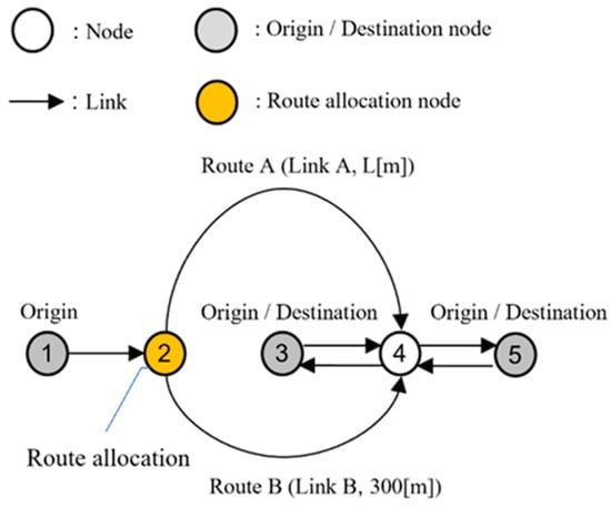
To study the feasibility of the cooperative route allocation system, we developed a simple traffic network, as shown in Figure 1. The network consists of nodes and links, which are described as $l$ and $m$, respectively. Additionally, we assumed that all the vehicles were CAVs connected to a cooperative route allocation system via communication. CAVs continuously provide the system with traffic information, such as their speed, position, and destination, and they can also receive instructions from the system.

Nodes 1, 3, and 5 are the origin nodes of the traffic flow, and Nodes 3 and 5 are the destination nodes. When vehicles flow into the network, the cooperative route allocation system, which is virtually installed on Node 2, allocates vehicles from Node 1 to either Route A or B. Both the routes consist of one link; the length of link B is 300 m and the variable length of Route A is denoted by $L$ m. The other links were set to 1000 m.

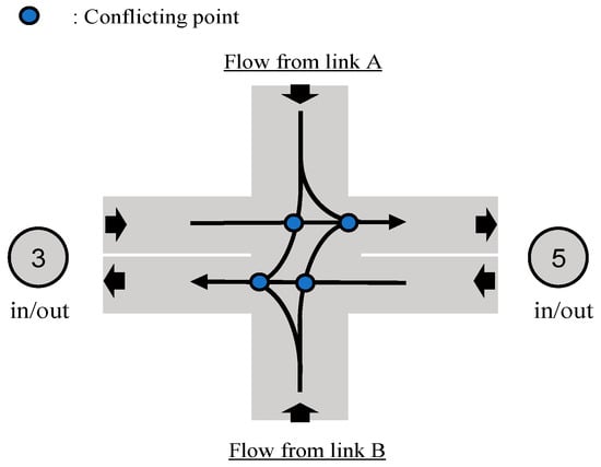
This system is able to constantly observe the traffic conditions of the entire network and allocate vehicles to their optimal routes to reduce the congestion at an intersection, which is described as Node 4. The target vehicles always travel along the route according to the system allocation and exit through Node 4 onto a route in the direction of the destination node. Figure 2 shows the shape of an intersection and the conflicting points at Node 4, where the paths of the turning traffic flows entering the intersection from Routes A/B and exiting to Nodes 3/5 intersect within the intersection, with straight traffic flows in both directions between Nodes 3 and 5.

For instance, the traffic originating from Node 1 and heading toward Node 5 is more likely to flow into Node 4 from Route A and turn left rather than enter from Route B and turn right, primarily because this avoids it crossing with the straight traffic flow from Node 5 to Node 3.

However, if the length of Route A is longer than that of Route B, irrespective of whether Route A has a longer travel distance, but fewer route crossings, or Route B has a shorter travel distance, but more route crossings, the faster link depends on the time required for each route and the presence or absence of a delay due to intersection crossings, a difference that varies depending on the situation. Therefore, we developed a dynamic route allocation system that considers the traffic conditions in the surrounding area, and we constructed a dynamic system–optimal planning model that allows for the allocation of vehicles to routes with non-minimal travel times considering the smoothness of the subsequent traffic flow. In the context of the transportation field, the system optimum is mainly used to set up problems aimed at minimizing the total travel time rather than equability among travelers. In addition, we built a mesoscopic traffic flow simulator to construct and validate the model.

3.2. Traffic Flow Simulation

To represent intersection conflict phenomena, the positions of the vehicles and the timing of their entries into the intersection must be represented separately.

We assumed that all the vehicles were CAVs so that we did not need to consider the stochastic behaviors in human-driven vehicles, such as random braking. Therefore, to reduce the computational load, the vehicle speed was only updated when a vehicle entered a new link or was forced to stop at the end of a link due to a conflict. In other words, the vehicles maintained a constant speed while traveling along a given link.

3.2.1. Vehicle Generation

Vehicles were generated during the first 9 min of the simulation, and model control was applied to vehicles departing from Node 1 within the first 6 min.

When the traffic volume from Node $1$ to Node $n$ was denoted by $x_{1n}$ vehicles/6 min, the total traffic volume generated from Node 1 was expressed as $X({=x}_{13}+x_{15})$ vehicles/6 min (equal to the number of vehicles controlled by the model). The branching rate at Node 3 was defined as $Y=x_{13}/X$% and was set to 50%. To satisfy X and Y, vehicles were given departure times and destinations, and each vehicle entered the network at its departure time. The traffic volume from Nodes 3 to 5 was constant at 60 vehicles/6 min (the same volume generated for Nodes 5–3), and vehicles were also given departure times.

3.2.2. Updating Vehicle Position and Speed

Each vehicle is described as $i$, and the position and speed of vehicle $i$ are denoted by $x_i$ and $v_i$, respectively. The vehicle position was updated using the following equation:

$$x_i^{t+1}=x_i^t+v_i^l$$

(1)

where $t$ is the simulation timestep, $x_i^t$ is the position of vehicle $i$ at timestep $t$, and $v_i^l$ is the speed of vehicle $i$ in link $l$.

When vehicle $i$ is generated and flows into the first link or moves to the next link at timestep $t$, the speed $v_i^l$ is determined by the average vehicle speed of link $l$ at timestep $t$, calculated using the equation proposed by Greenshield [44]:

$$v_i^l=v_{max}^l\left(1-{\displaystyle \frac{k_t^l}{k_j^l}}\right)$$

(2)

where $v_{max}^l$ is the maximum speed on link $l$, $k_t^l$ is the traffic density on link $l$ at timestep $t$, and $k_j^l$ is the maximum traffic density on link $l$. We assumed the average length of a standard car (4–5.5 m) and a minimal vehicle gap (2.5 m) so that the length occupied by one vehicle in the link was set to 8.0 m. Link B was the only link to possess two lanes, while the other links possessed one. Therefore, the maximum traffic density ($k_j^l(l\ne B)$) was 125 vehicles/km for all the links, and $k_j^B$ was set to 250 vehicles/km. Additionally, the maximum speed of all the links was set to 50 km/h, the typical maximum speed of urban traffic roads.

Furthermore, we assumed that the time required for the vehicle to decide its behavior in the next timestep from the surrounding information, including delays caused by communication, was up to one second. Hence, the simulation timestep ($t$) was set to one second.

3.2.3. Rules for Link Transition at Node 4

When a vehicle arrives at the end of link A/B, if it can transition to one link according to the following link transition rules, then the link transition is performed at the timestep at which the vehicle arrives. In this research, we assumed a future environment wherein all vehicles are CAVs, and we used the autonomous intersection control introduced in Section 1 instead of traffic signals. Thus, when multiple vehicles with intersecting trajectories attempt to enter an intersection simultaneously, the vehicle that is allowed to perform a link transition is determined based on the priority/non-priority or first-come, first-served (FCFS) rule to prevent collisions. The use of a more advanced intersection control is a subject for future work.

The priority/non-priority rule (STOP sign control) is still widely adopted to control the flow of traffic from residential areas to arterial roads. Based on the priority level set for each link, the vehicles on higher-priority links are allowed to transfer their links. A vehicle is allowed to enter an intersection if it has a higher priority than it does at the end of the link and it has a gap of at least 3 s before it reaches the intersection inflow section; otherwise, it waits at the end of the link. However, if the priorities of the traveling links are the same, such as at intersections with opposite links, the order of priority is assumed to be straight ahead > left turn > right turn. In addition, links A/B were set as non-priority, and the link between Nodes 3 and 5 was set as a priority. The FCFS rule allows vehicles that arrive at an intersection earlier to enter the intersection first regardless of the priority of the link. This means that a vehicle with a shorter waiting time to enter an intersection is given priority. However, if two or more vehicles with equal waiting times attempt to enter the intersection simultaneously, then the priority/non-priority rule is applied.

3.2.4. Waiting Queue Representation

Each vehicle is represented discretely. In contrast, the physical length of the waiting queue at an intersection is not considered owing to the reduced calculation load. We used a vertical queue to represent the waiting queues. A vehicle joining the queue was added to the top of the vertical stacking, and the vehicles at the bottom of the queue were sequentially drained to the intersection. The vehicles in the queue did not change their order (overtake), and the time required for one vehicle to flow out of the link was assumed to be 3 s. Hence, the maximum outflow rate of the link edge was one vehicle per 3 s.

All vehicles in the waiting queue were included in the calculation of the traffic density such that the presence of more vehicles in the waiting queue caused a lower average speed at a given link.

4. Establishment of Dynamic Route Allocation Model

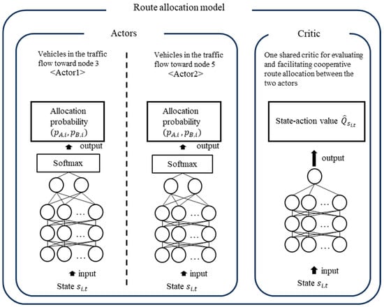
To realize the proposed cooperative route allocation system, we built a framework for a dynamic route allocation model using multiagent reinforcement learning. In general, reinforcement leaning is a method that heuristically searches for the optimal action that maximizes the reward that can be obtained by the agent in an environment based on a large number of simulations. In this framework, we referred to the actor–critic technique for the model construction, which is among the most well-known reinforcement learning techniques. In the actor–critic method, the models are divided into an actor model that makes decisions for an agent and a critic model that evaluates the actor’s decisions.

Figure 3 shows the structure of cooperative route allocation models. The actor is a neural network that comprises an input layer, two hidden layers that each consist of 128 nodes, and an output layer. The nodes between the layers are fully connected, and a rectified linear unit is used as the activation function for connections between the nodes, performing vehicle route allocation based on the observed traffic information. The number of nodes in the input layer corresponds to the length of the observed traffic data, while the output layer consists of two nodes, with one representing the allocation values for Route A and the other representing those for Route B. These values are then transformed into allocation probabilities for Routes A and B using the softmax function, ensuring that their sum equals 1. During the model’s training process, vehicles are randomly allocated to either Route A or B based on the allocation probabilities obtained by the actor. In contrast, during the validation phase, the vehicles are deterministically allocated to the route with the higher probability.

The critic is a neural network with the same structure as the actor except that its output layer consists of only a single node. The critic is used to predict the state–action value. The state–action value represents the value of the actor’s allocation in a given traffic state and is derived via backcalculation from the overall reward, which is based on the total travel time of all the vehicles after they reach their destinations. During the learning process, the critic is trained to accurately predict this state–action value, and the actor adjusts its allocation probabilities to take actions that are estimated by the critic to have higher value.

The agents were set up for each origin–destination pair of traffic flows in the target one-origin and two-destination traffic flows. Each of these agents was equipped with a distinct actor and was trained to allocate the vehicles within its assigned traffic flow to the optimal route, thereby maximizing the reward. However, the actors were not trained individually to minimize the total travel times of their respective traffic flows; instead, they were trained to consider cooperative behavior, enabling a reduction in the overall travel time of the target traffic flow.

To enable the actors to consider cooperative behavior, we developed a cooperative allocation model based on the framework proposed by Lowe et al., a well-established method in multiagent learning [45]. In Lowe’s framework, multiple agents share the impacts of their chosen actions in the critic’s evaluation. Consistent with the existing research, we aimed to foster cooperative behavior between the agents by having two actors share a single critic and receive combined rewards through the management of their respective traffic flows.

4.1. Simulation and Learning Flow

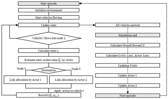
Figure 4 shows the learning flow, which includes the traffic simulation flow. First, we initialized the traffic network as a situation wherein all vehicles were waiting to flow into the network. We then started the simulation and advanced the timestep by updating the vehicle position and speed following the rules described in Section 3. Each vehicle had a predetermined departure time, origin node, and destination node, and flowed into its first link at its departure time. The departure times provided to the vehicles were randomly determined before the start of the training and did not change over the multiple simulations used to train the model.

The simulation continued until all the vehicles arrived at their destinations. The total travel and stop times and number of conflicts in the target traffic flow were recorded at the end of the simulation. Finally, we calculated the reward from the simulation results and updated the model parameters. This sequence of processes was defined as one episode that occurred during the learning process, and all the data obtained from an episode were used as one epoch.

4.2. Route Allocation Through Actors

During the simulation, when vehicle $i$, originating from Node 1, arrived at Node 2 at time step $t$, the actor allocated it to Route A or B. An entire traffic network state $s_{i,t}$ was calculated and input into the actor model, which consisted of four indicator values aggregated at intervals of 10 m from the beginning to the end of all routes: the traffic density (vehicles/m), average speed (km/h), number of vehicles heading to Node 3, and number of vehicles heading to Node 5.

The allocation probabilities ($p_{A,i}$,$p_{B,i}$) and the state–action value ($Q_{s_{i,t}}$) were estimated using the following equation:

$$p_{a,k}={\displaystyle \frac{e^{{\pi }_a\left(s_{i,t}\right)}}{{\sum }_a{e}^{{\pi }_a\left(s_{i,t}\right)}}}$$

(3)

$${\widehat{Q}}_{s_{i,t}}=\theta (s_{i,t})$$

(4)

where π is the policy value estimation function, and θ is the state–action value estimation function, which is approximated by each neural network. The vehicles were randomly allocated according to the following probabilities: $p_{A,k}$,$p_{B,k}$ were obtained from the actor. ($a$ = A: allocate vehicle $i$to Route A; $a$ = B: allocate vehicle $i$to Route B). Simultaneously, the traffic state ($s_{i,t}$), selection probability ($p_{a,i}$) of the adopted route, and state–action value ($Q_{S_{i,t}}$) estimated using the critic were recorded.

4.3. Reward Calculation

In the reinforcement learning, the simulation was executed while the agent performed the route allocation control and state–action value estimation, as described previously, and the parameters of the model (actor/critic) were updated to minimize the error ($\delta$) between the true state–action value ($Q$) and state–action value estimated by the critic ($\widehat{Q}$).

When the number of vehicles allocated by the model was $z_{max}$, the overall reward ($U$) was calculated using the following equation:

$$U={\displaystyle \frac{1}{100}}\left(c-{\displaystyle \sum _{z=1}^{z_{max}}}(f_z+d_z·w)\right)$$

(5)

where $f_z$ is the travel time of the $z$th controlled vehicle in an episode, $d_z$ is the waiting time to enter Node 4, $w$ is the weight assigned to the waiting time, and $c$ is an arbitrary constant. In related research, the travel and waiting times are not distinguished in the reward. We set the rewards as in Equation (4) to accommodate the case in which the model was trained to focus more on reducing delays due to conflicts.

The reward ($R_z$) obtained via the allocation of the $z$th vehicle is given by the overall reward (U), as follows:

$$\begin{gathered} R_z=U,\hspace{1em}z=z_{max} \\ {R}_{z-1}=R_z·{\gamma }^{d{t}_{z-1,z}},\hspace{1em}2<z<z_{max} \end{gathered}$$

(6)

where $\gamma$(=0.99) is the discount factor, and $d{t}_{z-1,z}$ is the time interval between the ($z-1$)th and $z$th vehicles. The overall reward (U) is reflected in the reward obtained via the allocation of each vehicle, which thereby allows the model to determine the allocation of each vehicle so that the future rewards are larger.

General reinforcement learning tasks assume that agents act at regular intervals. However, in this research, the agent acted during each influx of vehicles into the branching node, and the intervals were not constant. Thus, the discounting of rewards according to the time interval per action is represented by ${\gamma }^{d{t}_{z-1,z}}$ in Equation (6).

4.4. Updating Model Parameters

The reward for allocating the $z$th vehicle ($R_z$) is the true state–action value of $Q_z$. Here, when $\widehat{Q_z}$ is defined as the estimated state–action value, the estimation error (${\delta }_z$) made by the critic is given as follows:

$${\delta }_z={\widehat{Q}}_z-Q_z$$

(7)

Then, the $Critic Los{s}_z$ is calculated using the smooth_f1_loss function, which is commonly used as an objective function for neural network parameter optimization:

$$Critic Los{s}_z=\left\{\begin{array}{c}{\displaystyle \frac{1}{2}}{\delta }_z^2, \left|{\delta }_z\right|<1\\ {\delta }_z-{\displaystyle \frac{1}{2}},\left|{\delta }_z\right|>1\end{array}\right.$$

(8)

Further, the $Actor Los{s}_z$ is obtained from the following equation:

$$Actor Los{s}_z=-\log \left(p_{a,z}\right){\delta }_z,$$

(9)

where ${ p}_{a,z}$ is the allocation probability of the selected action ($a$) for vehicle $z$.

The critic loss and actor loss were used to update the model parameters for the critic and actor, respectively. The AdamW [46] algorithm was used to optimize the model, and the learning rate was set to 0.0001.

4.5. Experiment Settings

The reinforcement learning framework and traffic flow simulator explained in Section 3.2 were coded in the Python programming language. Additionally, we utilized the tensor calculation library PyTorch to implement the model structure and update the model parameters. To investigate the impact of cooperative route allocation under various traffic conditions, the models were trained and validated under several traffic conditions. The model training was performed by changing four operational variables—the traffic volume from Node 1 ($X$) (vehicles/6 min); the length of Route A $\left(L\right)$ (m); the control method of the intersection at Node 4; and the weight for the waiting time ($w$) in the reward.

Table 1. Options for each traffic condition variable.

Traffic Condition Variable	Options
$\mathrm{Traffic} \mathrm{volume} \mathrm{from} \mathrm{Node} 1 (X$) (vehicles/6 min)	80 or 120 vehicles/6 min
$\mathrm{Length} \mathrm{of} \mathrm{Route} \mathrm{A} \left(L\right)$(m)	450 or 600 m
$\mathrm{Weight} \mathrm{for} \mathrm{waiting} \mathrm{time} (w$) in the reward	1.0 or 5.0
Control method of the intersection at Node 4	Priority/non-priority or first-come, first-served control

shows the options for each traffic situation variable. The traffic volume from Node 1 ($X$) was set to 80 or 120 vehicles/6 min (800 or 1200 vehicles/h). These values were set to replicate a medium-scale traffic flow, referencing the maximum traffic capacity of 2200 pcu/h for a one-lane road among Japan’s standard traffic road capacities. The lengths of Route A were set to be longer than those of Route B, with options of 450 m and 600 m. As discussed in Section 3, this configuration was used to investigate whether selecting the longer Route A over the shorter Route B, considering intersection conflicts, improved the overall efficiency. Additionally, we examined the impact on the allocation tendency of treating the stop time in the reinforcement learning reward as-is versus increasing its weight. Furthermore, we analyzed how the differences in the ease of entry into the intersection from Route A or Route B, arising from the use of two distinct intersection entry rules, influenced the allocation.

Experiments were conducted under 16 traffic conditions that combined all of these variables. A total of 20,000 episodes were performed for each traffic condition, and one model was constructed for each condition.

5. Results and Discussion

We analyzed the model-training process and the allocation results obtained by the trained model. During the training process, we calculated the average travel time of the vehicle, the average number of conflicts, and the average waiting time for each episode, and we further recorded the average of these values for every 100 episodes. Conflicts were defined as situations wherein a vehicle was prevented from entering an intersection due to the presence of a higher-priority vehicle in the simulation. The number of conflicts at Node 4 was recorded for each vehicle. However, if one vehicle simultaneously conflicted with multiple vehicles at the same time, the number of conflicts was counted as the number of vehicles in the conflict.

5.1. The Training Process

5.1.1. First-Come, First-Served Rule

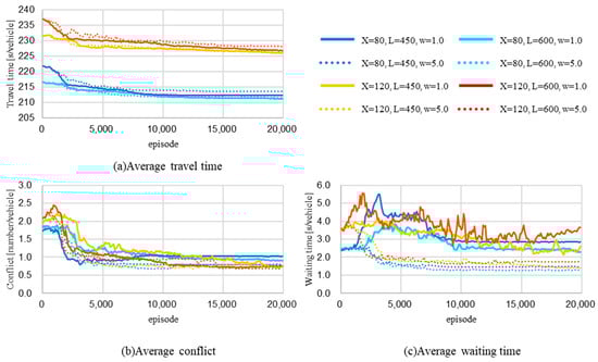
Figure 5 shows the results of the model training when the FCFS rule was implemented. The upper left figure (a), lower left figure (b), and lower right figure (c) represent the trends of the average travel time, average number of conflicts, and average waiting time, respectively.

First, in all cases, the average travel time of the vehicle decreased compared to the initial training phase. Depending on the volume of traffic from Node 1 (the traffic to be controlled) (X), the average travel time was divided into two categories, both of which exhibited large decreases within the first 5000 episodes and gradual decreases thereafter. The length of Route A and the waiting time weight had slight impacts on the results, and the process of decreasing the travel time was nearly identical in all cases.

The average number of conflicts decreased in all cases. In several cases ($X$ = 120 vehicles/6 min), the number of conflicts increased within the first training phase; however, the average number of conflicts per vehicle was reduced by approximately one-half of that in the initial phase in all cases.

The waiting times differed from the conflict and travel times, and the results significantly varied depending on the waiting time weight ($w$). In the cases wherein $w$ was 5.0, the average waiting time of the vehicles exhibited a decreasing trend. However, in most cases, where $w$ was 1.0, the waiting time increased significantly in the early episodes and then increased and decreased repeatedly; however, the final value was higher than the initial value. Nevertheless, because the average waiting time was only a few seconds, which was a small percentage of the trip time, the average travel time decreased even in cases where the waiting times increased.

5.1.2. The Priority/Non-Priority Rule

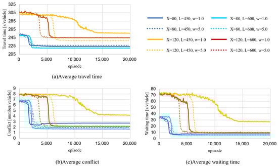
Figure 6 shows the training results for the priority/non-priority (P/NP) rule, as shown in Figure 5. Notably, the vertical axis ranges in Figure 6 are different from those in Figure 5.

In the results for the P/NP rule, there is a strong similarity between the decreasing travel time, the number of conflicts, and the waiting time. In the simulation, the conflict at Node 4 caused a waiting queue on Routes A and B and this congestion further resulted in an increase in the travel time of the target traffic flow. According to the P/NP rule, the vehicles on Routes A/B had a lower priority for intersection entry; therefore, waiting queues were more likely to occur under this rule than under the FCFS rule. In fact, the number of conflicts in the P/NP cases was more than twice that in the FCFS cases, and the waiting time of the initial phase was several tens of seconds with the P/NP rule compared to a few seconds with the FCFS rule. Thus, there may be similarities among the observations due to the high importance of conflicts that caused congestion in the reduction in the travel time in the P/NP cases.

In all cases, except for the case in which $X$ was 120 vehicles/6 min, $L$ was 450 m, and $w$ was 1.0, the number of conflicts decreased rapidly within a few hundred episodes and then converged to a constant value. The waiting time weight ($w$) affected the cases wherein $X$ was 120 vehicles/6 min, reduced the number of conflicts for the case wherein $X$ was 120 vehicles/6 min, L was 450 m, and $w$ was 5.0, and converged faster and to smaller values than when w was 1.0.

Additionally, when X was 120 vehicles/6 min, L was 600 m, and $w$ was 5.0, the waiting time converged faster than for the case wherein w was 1.0. However, the conflict reduction was almost the same for both cases, and the waiting and travel times showed decreasing trends.

5.2. Model Validation

Test simulations were conducted to evaluate the differences in the model allocation trained under several different traffic settings. Each model was validated using a simulation with the same setting as the environment in which it was trained, and the travel times and allocated routes of the controlled vehicles were recorded. Additional simulations were conducted, wherein random allocations were made such that the allocation percentages of the routes for each destination were the same as the results from the model. For instance, if the traffic flow toward Node 5 allocated 50% of the vehicles to Route A and the rest to Route B, random allocation maintained this allocation percentage while randomly determining the allocation routes for each vehicle. Because the traffic conditions were identical and the departure time of each vehicle was the same, a paired t-test could be applied to compare the model and random allocation results. The following equation was used as the test statistic:

$$u={\displaystyle \frac{1}{n}}{\displaystyle \sum _{z=1}^{z_{max}}}\left(F_z^{\prime }-F_z\right)$$

(10)

where $u$ is the average travel time reduction for the model allocation compared to the random allocation; $F_z(=f_z+d_z)$ is the travel time of vehicle $z$ in the model allocation simulations; $F_z^{\prime }$ is a random allocation; and $z_{max}$ is the total number of allocated vehicles. In the random simulation, ten simulations with different random number generation seeds were performed, and all the data were used for the test. The null hypothesis was that $z$ was greater than zero. The results of the t-test and allocation percentages of the model-applied simulations are presented in

Table 2. Allocation results from trained models.

X [vehicles/6 min]	L [m]	w	Rules Installed at Node 4	Allocation Percentage for Traffic Flow Toward Node 5 [%]		Allocation Percentage for Traffic Flow Toward Node 3 [%]		Average Waiting Time of Model Allocation [s/vehicle]	Average Travel Time of Model Allocation [s/vehicle]	Average Waiting Time of Random Allocation [s/vehicle]	Average Travel Time of Random Allocation [s/vehicle]	Average Travel Time Reduction [s/vehicle]
				Route A	Route B	Route A	Route B
80	450	1	FCFS	12.5	87.5	10.0	90.0	2.14	211.1	5.20	214.7	3.63 *
80	600	1	FCFS	17.5	82.5	0.00	100	2.85	212.2	4.43	214.6	2.35 *
80	450	5	FCFS	50.0	50.0	2.50	97.5	1.30	211.5	2.50	212.8	1.28 *
80	600	5	FCFS	35.0	65.0	2.50	97.5	1.48	213.5	3.28	214.9	1.42 *
120	450	1	FCFS	40.0	60.0	0.00	100	2.56	225.6	3.99	227.3	1.71 *
120	600	1	FCFS	25.0	75.0	0.00	100	3.58	226.6	7.54	232.6	5.99 *
120	450	5	FCFS	70.0	30.0	0.00	100	1.40	226.1	2.61	227.7	1.61 *
120	600	5	FCFS	51.7	48.3	0.00	100	1.75	228.2	2.65	229.7	1.52 *
80	450	1	P/NP	100	0.00	0.00	100	5.88	219.8	5.88	219.8	-
80	600	1	P/NP	62.5	37.5	0.00	100	7.90	223.2	46.4	260.0	36.8 *
80	450	5	P/NP	90.0	10.0	12.5	87.5	6.01	220.2	25.0	239.1	18.9 *
80	600	5	P/NP	92.5	7.50	15.0	85.0	5.81	226.8	25.5	245.9	19.2 *
120	450	1	P/NP	83.3	16.7	13.3	86.7	27.0	255.5	68.5	296.4	40.9 *
120	600	1	P/NP	100	0.00	0.00	100	9.73	244.7	9.73	255.5	-
120	450	5	P/NP	100	0.00	0.00	100	9.42	237.9	9.42	244.7	-
120	600	5	P/NP	100	0.00	0.00	100	9.73	244.7	9.73	237.9	-

X: traffic volume flow from Node 1 (vehicles/6 min); L: length of Route A (m); w: weight of waiting time in reward formulation; FCFS: first-come, first-served; P/NP: priority/non-priority. Comparisons could not be made because there was no difference between the model and random allocation. *: p < 0.01.

.

5.2.1. Model Trained with First-Come, First-Served Rule

According to the allocation percentages of the models trained with the FCFS rule, almost all the vehicles in the traffic flow toward Node 3 were allocated to Route B. As shown in Figure 2, the traffic flow toward Node 3 made a left turn at the intersection, resulting in fewer conflict points in the intersection trajectory. In addition, because Route B was shorter than Route A, a majority of the vehicles were allocated to Route B, which was faster and less conflicting. However, the allocation of vehicles toward Node 5 varied depending on the traffic settings. The allocation balance for each route varied depending on $X$, $L$, and $w$.

These findings may be attributed to the relationship between the number of vehicles on a route and the average speed, as expressed in Equation (1). For instance, when there are fewer vehicles on Route B and less time is required to pass through it, the vehicles traveling to Node 5 may prefer to pass through Route B, which is shorter, allowing for a delay owing to conflicts. However, as the number of vehicles allocated to Route B increases, the time required to traverse Route B increases and eventually becomes identical to that of Route A, which is longer. The FCFS rule, which has a negligible effect on the delay owing to conflicts, resulted in an allocation that placed importance on the time required to pass through the route.

The model trained with the FCFS rule exhibited significantly shorter travel times in all cases compared to the results with random allocation, which implies that the model can appropriately select the allocation route according to the traffic conditions surrounding each vehicle.

5.2.2. Model Trained with Priority/Non-Priority Rule

According to the allocation trend for the P/NP rule, most of the traffic flow toward Node 5 was allocated to Route A and most of the traffic flow toward Node 3 was allocated to Route B because the delay effects caused by conflicts are substantial in the P/NP rule, and the vehicles were allocated to routes with fewer conflict points at Node 4, according to their destinations, to form traffic flows in which conflicts were less likely to occur.

In some cases, the allocation routes were completely separated according to the destination. In these cases, there was no difference between the model and random assignments owing to random allocation. However, the allocation percentage should be the same as the model allocation. Therefore, excluding these cases, we compared the travel times and found that the travel times in the simulation with model allocation were significantly shorter than those in the simulation with random allocation.

5.2.3. Impact of Weights for Stop Times on Results

The weights for the waiting times worked in the FCFS rule in the training. If $X$ and $L$ are the same, the average travel time of model allocation for both, despite the different $w$ values, are similar. A model trained with a weight of five resulted in shorter waiting times than when using a model trained with a weight of one. However, for the priority/non-priority rule, the weights did not work as well as they were shown to in the results for the FCFS rule. Owing to the large impact of the waiting time on the travel time, the model was trained to reduce the waiting time, even when w was 1.0. However, in the cases of $X$ = 120 and $L$ = 450, the weights had an effect: the model trained with $w$ = 1.0 had an average stop time of 27 s, which is a larger value compared to the result with weights of 5.0, and a longer average travel time. When w was 1.0, maximizing the reward implied minimizing the average travel time. Nevertheless, in these two cases, the model trained at w = 5.0 had a shorter average time; therefore, we expected the model to converge to a locally optimal solution when training at $w$ = 1.0.

5.3. Additional Experiment Using More Congested Traffic

In the cooperative allocation using the FCFS rule, the waiting time proportion in the total vehicle travel time was small. Consequently, additional model training and validation were conducted under increased traffic volumes, leading to more congestion at the intersection. The traffic volume from Node 1 was set to 1600 vehicles per hour, while the traffic volume between Nodes 3 and 5 was set to 800 vehicles per hour.

Table 3. Allocation results from trained models.

X [vehicles/6 min]	L [m]	w	Rules Installed at Node 4	Allocation Percentage for Traffic Flow Toward Node 5 [%]		Allocation Percentage for Traffic Flow Toward Node 3 [%]		Average Waiting Time of Model Allocation [s/vehicle]	Average Travel Time of Model Allocation [s/vehicle]	Average Waiting Time of Random Allocation [s/vehicle]	Average Travel Time of Random Allocation [s/vehicle]	Average Travel Time Reduction [s/vehicle]
				Route A	Route B	Route A	Route B
160	450	1	FCFS	73.8	26.2	0.00	100	3.19	258.0	7.55	263.0	4.93 *
160	600	1	FCFS	62.5	37.5	0.00	100	4.64	262.7	10.7	269.3	6.63 *
160	450	5	FCFS	100	0.00	0.00	100	3.03	260.7	3.03	260.7	-
160	600	5	FCFS	100	0.00	0.00	100	3.15	268.2	3.15	268.2	-

X: traffic volume flow from Node 1 (vehicles/6 min); L: length of Route A (m); w: weight of waiting time in reward formulation; FCFS: first-come, first-served. Comparisons could not be made because there was no difference between model and random allocation. *: p < 0.01.

presents the results of the model validation, conducted in the same manner as in Table 2. When compared to the allocation results under the medium-scale traffic volume shown in Table 2, the increased traffic volume resulted in a higher allocation of vehicles to Route A in the traffic flow toward Node 5, suggesting that even under the FCFS rule, as the number of vehicles entering the intersection increases and congestion becomes more likely, the model learns to allocate the vehicles to routes with fewer conflicts at the intersection. Specifically, when the waiting time weight (w) was set to 5, the routes assigned to the vehicles were completely separated based on their destinations, providing additional evidence for the previous discussion regarding the impact of the stop time weight in the reward function on the allocation results. This result supports our initial assumption that cooperative route allocation, which reduces conflicts under high-inbound-traffic conditions at intersections, is necessary to assist intersection management systems. Additionally, through installing future intersection management systems, as introduced in Section 1, further reductions in the travel and waiting times can be achieved.

However, the design of the waiting time weight in the reward function requires additional discussion in future work. When compared to the results with w = 1, the model’s average waiting time was similar or slightly smaller, while the travel time was slightly higher. While reducing the waiting time is effective at decreasing the total travel time, it does not necessarily guarantee its minimization.

6. Conclusions

Many methods have been developed to efficiently avoid vehicle conflicts at intersections in future CAV traffic environments by controlling vehicle acceleration and deceleration; however, few approaches have used route planning. Although the related research includes intersection conflicts in traffic behavior modeling, the evaluation metrics focus only on the travel time and do not include the number of conflicts or the waiting time. Thus, we devised a cooperative route allocation system that primarily focuses on vehicle waiting times due to intersection congestion. A simple traffic network was constructed and a dynamic route allocation model was trained using reinforcement learning. In the reward function, the vehicle travel and waiting times were separately represented, including the waiting time weight, to investigate how significantly the waiting time affected the traffic flow efficiency. The trained model could make appropriate allocations that reduced conflicts, as well as the travel and waiting times.

The model allocation results indicate that it is possible to reduce the average trip time by selecting routes that reduce the number of conflict points in the trajectories at intersections depending on the destination. However, these allocation results may vary depending on the degree to which delays due to conflicts affect the traffic flow. At intersections with priority/non-priority control, where conflicts have a greater impact on the traffic flow, some vehicles are forced to take a long time to reduce conflicts at the intersection.

This study has two major limitations. The first is the simplicity of the traffic networks. There were only two possible routes for allocation and two destinations for the target traffic flow. While our findings are applicable to some limited traffic network areas, such as expressways, further improvement is needed to achieve our final goal of building a route planning system for the entire urban transportation network, which is a complex network that possesses countless destinations depending on the trip. Therefore, investigating the feasibility of using the proposed method in extended networks by referring to real traffic networks and volumes is necessary. The second limitation is related to reinforcement learning. During the training of our model, the vehicle departure times were the same throughout the episode. Therefore, the constructed model is not highly effective in situations with different departure times. Model generalization is a universal challenge in reinforcement learning, and it must be addressed to make this approach feasible for complex traffic flows.

Finally, we discuss further improvements to this research. We focused on vehicle travel and waiting times in the construction and validation of our model. Traffic efficiency not only reduces travel time but also has the potential to reduce energy consumption, contributing to the realization of sustainable transportation. Additionally, reducing intersection conflicts enhances traffic safety. Therefore, in order to adopt a more comprehensive approach to cooperative allocation, we aim to incorporate not only the travel time but also energy consumption and safety indicators into the reinforcement learning reward function, allowing for the consideration of a broader set of perspectives.

Another improvement to this study would be to apply route allocation learning in tandem with intersection control methods for CAVs. Our goal is to build a comprehensive vehicle travel control system for future traffic flows with a nearly 100% CAV penetration rate. Therefore, consideration of the synergistic effects of conflict avoidance using a novel intersection management system and route planning is necessary. However, the validation of the established systems requires a simulator that can accurately reproduce real-world traffic flows and a detailed definition of automated driving and communication technology.

References

- Sun, D.; Zhang, C.; Zhang, L.; Chen, F.; Peng, Z.-R. Urban travel behavior analyses and route prediction based on floating car data. Trans. Lett. 2014, 6, 118–125. [Google Scholar] [CrossRef]
- Feng, Y.; Hourdos, J.; Davis, G.A. Probe vehicle based real-time traffic monitoring on urban roadways. Trans. Res. Part C Emerg. Technol. 2014, 40, 160–178. [Google Scholar] [CrossRef]
- Tashiro, M.; Motoyama, H.; Ichioka, Y.; Miwa, T.; Morikawa, T. Simulation analysis on optimal merging control of connected vehicles for minimizing travel time. Int. J. Intell. Transp. Syst. Res. 2020, 18, 65–76. [Google Scholar] [CrossRef]
- Dresner, K.; Stone, P. Multiagent traffic management: An improved intersection control mechanism. In Proceedings of the fourth International Joint Conference on Autonomous Agents and Multiagent Systems, Utrecht, The Netherlands, 25–29 July 2005; pp. 471–477. [Google Scholar] [CrossRef]
- Li, L.; Wang, F.Y. Cooperative driving at blind crossings using intervehicle communication. IEEE Trans. Veh. Technol. 2006, 55, 1712–1724. [Google Scholar] [CrossRef]
- Xu, B. Distributed conflict-free cooperation for multiple connected vehicles at unsignalized intersections. Transp. Res. C 2018, 93, 322–334. [Google Scholar] [CrossRef]
- Levin, M.W.; Rey, D. Conflict-point formulation of intersection control for autonomous vehicles. Transp. Res. C Emerg. Technol. 2017, 85, 528–547. [Google Scholar] [CrossRef]
- Liu, B.; Shi, Q.; Song, Z.; El-Kamel, A. Trajectory planning for autonomous intersection management of connected vehicles. Simul. Model. Pract. Theory 2019, 90, 16–30. [Google Scholar] [CrossRef]
- Chen, X.; Hu, M.; Xu, B.; Bian, Y.; Qin, H. Improved reservation-based method with controllable gap strategy for vehicle coordination at non-signalized intersections. Physical A 2022, 604, 127953. [Google Scholar] [CrossRef]
- Lee, J.; Park, B. Development and evaluation of a cooperative vehicle intersection control algorithm under the connected vehicles environment. IEEE Trans. Intell. Transp. Syst. 2012, 13, 81–90. [Google Scholar] [CrossRef]
- Zhang, Y.J.; Malikopoulos, A.A.; Cassandras, C.G. Optimal control and coordination of connected and automated vehicles at urban traffic intersections. In Proceedings of the 2016 American Control Conference (ACC), Boston, MA, USA, 6–8 July 2016; pp. 6227–6232. [Google Scholar] [CrossRef]
- Kamal, M.A.S.; Imura, J.; Ohata, A.; Hayakawa, T.; Aihara, K. ‘Coordination of automated vehicles at a traffic-lightless intersection. In Proceedings of the 16th International IEEE Conference on Intelligent Transportation Systems (ITSC), The Hague, The Netherlands, 6–9 October 2013; pp. 922–927. [Google Scholar] [CrossRef]
- Qian, X.; Gregoire, J.; de La Fortelle, A.; Moutarde, F. Decentralized model predictive control for smooth coordination of automated vehicles at intersection. In Proceedings of the 2015 European Control Conference (ECC), Linz, Austria, 15–17 July 2015; pp. 3452–3458. [Google Scholar] [CrossRef]
- Hult, R.; Zanon, M.; Gros, S.; Wymeersch, H.; Falcone, P. Optimisation based coordination of connected, automated vehicles at intersections. Veh. Syst. Dyn. 2020, 58, 726–747. [Google Scholar] [CrossRef]
- Medina, A.I.M.; Creemers, F.; Lefeber, E.; van de Wouw, N. Optimal access management for cooperative intersection control. IEEE Trans. Intell. Transp. Syst. 2020, 21, 2114–2127. [Google Scholar] [CrossRef]
- Scholte, W.J.; Zegelaar, P.W.A.; Nijmeijer, H. A control strategy for merging a single vehicle into a platoon at highway on-ramps. Transp. Res. C Emerg. Technol. 2022, 136, 103511. [Google Scholar] [CrossRef]
- Fayazi, S.A.; Vahidi, A.; Luckow, A. Optimal scheduling of autonomous vehicle arrivals at intelligent intersections via MILP. In Proceedings of the 2017 American Control Conference (ACC), Seattle, WA, USA, 24–26 May 2017; pp. 4920–4925. [Google Scholar] [CrossRef]
- Ashtiani, F.; Fayazi, S.A.; Vahidi, A. Multi-intersection traffic management for autonomous vehicles via distributed mixed integer linear programming. In Proceedings of the 2018 Annual American Control Conference (ACC), Milwaukee, WI, USA, 27–29 June 2018; pp. 6341–6346. [Google Scholar] [CrossRef]
- Fayazi, S.A.; Vahidi, A. Vehicle-in-the-loop (VIL) verification of a smart city intersection control scheme for autonomous vehicles. In Proceedings of the IEEE Conference on Control Technology and Applications (CCTA), Maui, HI, USA, 27–30 August 2017; pp. 1575–1580. [Google Scholar] [CrossRef]
- Wu, Y.; Chen, H.; Zhu, F. DCL-AIM: Decentralized coordination learning of autonomous intersection management for connected and automated vehicles. Transp. Res. C Emerg. Technol. 2019, 103, 246–260. [Google Scholar] [CrossRef]
- Isele, D. Navigating occluded intersections with autonomous vehicles using deep reinforcement learning. arXiv 2017, arXiv:1705.01196. [Google Scholar]
- Guo, Z.; Wu, Y.; Wang, L.; Zhang, J. Coordination for connected and automated vehicles at non-signalized intersections: A value decomposition-based multiagent deep reinforcement learning approach. IEEE Trans. Veh. Technol. 2023, 72, 3025–3034. [Google Scholar] [CrossRef]
- Chen, C.; Xu, Q.; Cai, M.; Wang, J.; Wang, J.; Li, K. Conflict-Free Cooperation Method for Connected and Automated Vehicles at Unsignalized Intersections: Graph-Based Modeling and Optimality Analysis. IEEE Trans. Intell. Transp. Syst. 2022, 23, 21897–21914. [Google Scholar] [CrossRef]
- Klimke, M.; Völz, B.; Buchholz, M. Cooperative Behavior Planning for Automated Driving Using Graph Neural Networks. In Proceedings of the 2022 IEEE Intelligent Vehicles Symposium (IV), Aachen, Germany, 4–9 June 2022; pp. 167–174. [Google Scholar] [CrossRef]
- Zhao, R.; Li, Y.; Gao, F.; Gao, Z.; Zhang, T. Multi-Agent Constrained Policy Optimization for Conflict-Free Management of Connected Autonomous Vehicles at Unsignalized Intersections. IEEE Trans. Intell. Transp. Syst. 2024, 25, 5374–5388. [Google Scholar] [CrossRef]
- Risser, R. Behavior in traffic conflict situations. Accid. Anal. Prev. 1985, 17, 179–197. [Google Scholar] [CrossRef]
- Gkyrtis, K.; Kokkalis, A. An Overview of the Efficiency of Roundabouts: Design Aspects and Contribution toward Safer Vehicle Movement. Vehicles 2024, 6, 433–449. [Google Scholar] [CrossRef]
- Lu, J.; Ren, C.; Shao, Y.; Zhu, J.; Lu, X. An automated guided vehicle conflict-free scheduling approach considering assignment rules in a robotic mobile fulfillment system. Comput. Ind. Eng. 2023, 176, 108932. [Google Scholar] [CrossRef]
- Xie, W.; Peng, X.; Liu, Y.; Zeng, J.; Li, L.; Eisaka, T. Conflict-free coordination planning for multiple automated guided vehicles in an intelligent warehousing system. Simul. Model. Pract. Theory 2024, 134, 102945. [Google Scholar] [CrossRef]
- Hu, H.; Yang, X.; Xiao, S.; Wang, F. Anti-conflict AGV path planning in automated container terminals based on multi-agent reinforcement learning. Int. J. Prod. Res. 2021, 61, 65–80. [Google Scholar] [CrossRef]
- Ni, X.-Y.; Sun, D.; Zhao, J.; Chen, Q. Two-Stage Allocation Model for Parking Robot Systems Using Cellular Automaton Simulation. Transp. Res. Rec. 2024, 2678, 608–622. [Google Scholar] [CrossRef]
- Bang, H.; Chalaki, B.; Malikopoulos, A.A. Combined Optimal Routing and Coordination of Connected and Automated Vehicles. IEEE Control. Syst. Lett. 2022, 6, 2749–2754. [Google Scholar] [CrossRef]
- Bang, H.; Malikopoulos, A.A. Re-Routing Strategy of Connected and Automated Vehicles Considering Coordination at Intersections. arXiv 2023, arXiv:2210.00396. [Google Scholar]
- Roselli, S.F.; Fabian, M.; Åkesson, K. Conflict-free electric vehicle routing problem: An improved compositional algorithm. Discret. Event Dyn. Syst. 2023, 34, 21–51. [Google Scholar] [CrossRef]
- Nazari, M.; Oroojlooy, A.; Snyder, L.V.; Takáč, M. Reinforcement learning for solving the vehicle routing problem. arXiv 2018, arXiv:1802.04240. [Google Scholar]
- Sun, N.; Shi, H.; Han, G.; Wang, B.; Shu, L. Dynamic Path Planning Algorithms with Load Balancing Based on Data Prediction for Smart Transportation Systems. IEEE Access 2020, 8, 15907–15922. [Google Scholar] [CrossRef]
- Zhou, C.; Ma, J.; Douge, L.; Chew, E.P.; Lee, L.H. Reinforcement Learning-based approach for dynamic vehicle routing problem with stochastic demand. Comput. Ind. Eng. 2023, 182, 109443. [Google Scholar] [CrossRef]
- Regragui, Y.; Moussa, N. A real-time path planning for reducing vehicles traveling time in cooperative-intelligent transportation systems. Simul. Model. Pract. Theory 2023, 123, 102710. [Google Scholar] [CrossRef]
- Yan, L.; Wang, P.; Yang, J.; Hu, Y.; Han, Y.; Yao, J. Refined Path Planning for Emergency Rescue Vehicles on Congested Urban Arterial Roads via Reinforcement Learning Approach. J. Adv. Transp. 2021, 2021, e8772688. [Google Scholar] [CrossRef]
- Koh, S.; Zhou, B.; Fang, H.; Yang, P.; Yang, Z.; Yang, Q.; Guan, L.; Ji, Z. Real-time deep reinforcement learning based vehicle navigation. Appl. Soft Comput. 2020, 96, 106694. [Google Scholar] [CrossRef]
- Guillen-Perez, A.; Cano, M.-D. Multi-Agent Deep Reinforcement Learning to Manage Connected Autonomous Vehicles at Tomorrows Intersections. IEEE Trans. Veh. Technol. 2022, 71, 7033–7043. [Google Scholar] [CrossRef]
- Joo, H.; Ahmed, S.H.; Lim, Y. Traffic signal control for smart cities using reinforcement learning. Comput. Commun. 2020, 154, 324–330. [Google Scholar] [CrossRef]
- Gregurić, M.; Vujić, M.; Alexopoulos, C.; Miletić, M. Application of Deep Reinforcement Learning in Traffic Signal Control: An Overview and Impact of Open Traffic Data. Appl. Sci. 2020, 10, 4011. [Google Scholar] [CrossRef]
- Greenshields, B.D. A study of traffic capacity. In Proceedings Highway Research Board; Highway Research Board: Washington, DC, USA, 1935; Volume 14, pp. 448–477. [Google Scholar]
- Lowe, R.; Wu, Y.; Tamar, A.; Harb, J.; Abbeel, P.; Mordatch, I. Multi-agent actor-critic for mixed cooperative-competitive environments. arXiv 2020, arXiv:1706.02275. [Google Scholar]
- Loshchilov, I.; Hutter, F. Decoupled weight decay regularization. arXiv 2019, arXiv:1711.05101. [Google Scholar]
Disclaimer/Publisher’s Note: The statements, opinions and data contained in all publications are solely those of the individual author(s) and contributor(s) and not of MDPI and/or the editor(s). MDPI and/or the editor(s) disclaim responsibility for any injury to people or property resulting from any ideas, methods, instructions or products referred to in the content. |
© 2024 by the authors. Licensee MDPI, Basel, Switzerland. This article is an open access article distributed under the terms and conditions of the Creative Commons Attribution (CC BY) license (https://creativecommons.org/licenses/by/4.0/).