Article

Virtual Validation and Uncertainty Quantification of an Adaptive Model Predictive Controller-Based Motion Planner for Autonomous Driving Systems

by
Mohammed Irshadh Ismaaeel Sathyamangalam Imran
*,
Satyesh Shanker Awasthi
,
Michael Khayyat
,
Stefano Arrigoni
* and
Francesco Braghin
Department of Mechanical Engineering, Politecnico di Milano, Via Giuseppe La Masa, 1, 20156 Milano, Italy
*
Authors to whom correspondence should be addressed.
Future Transp. 2024, 4(4), 1537-1558; https://doi.org/10.3390/futuretransp4040074
Submission received: 12 July 2024 / Revised: 31 October 2024 / Accepted: 5 November 2024 / Published: 2 December 2024

Abstract

In the context of increasing research on algorithms for different modules of the autonomous driving stack, the development and evaluation of these algorithms for deployment onboard vehicles is the next critical step. In the development and verification phases, simulations play a pivotal role in achieving this aim. The uncertainty quantification of Autonomous Vehicle (AV) systems could be used to enhance safety assurance and define the error-handling capabilities of autonomous driving systems (ADSs). In this paper, a virtual validation methodology for the control module of an autonomous driving stack is proposed. The methodology is applied to a rule-defined Model Predictive Controller (MPC)-based motion planner, where uncertainty quantification (UQ) is performed across various scenarios, based on the intended functionality within the algorithm’s operational design domain (ODD). The framework is designed to assess the performance of the algorithm under localization uncertainties, while performing obstacle vehicle-overtaking, vehicle-following, and safe-stopping maneuvers.

1. Introduction

Highly Automated Driving (HAD) vehicles, classified as Level 3 and above in the SAE J3016 standard [1], remove the human driver from the direct control loop. This shift creates the need to homologate the AV’s driving functions rather than the driver. Proving the reliability of ADSs solely through on-road testing is insufficient, as it would require millions of miles of driving to statistically ensure safety and account for all scenarios, including edge and corner cases [2,3]. As a result, simulation-based testing has become essential for validating ADSs, forming the backbone of standardization efforts [4]. The lack of fidelity in virtual validation could be addressed once the virtual testing tool chain itself has been validated [5]. The UNECE-R157 regulation, a landmark in harmonized regulatory frameworks for HAD systems [6], outlines type approval guidelines for Automated Lane Keeping Systems (ALKSs). It is also the primary regulation to consider simulation and mathematical models as integral parts of the verification and validation tool chain. Simulations were used to define collision avoidance conditions for ALKSs, considering parameters such as initial and relative velocities between the ego and obstacle vehicles, as well as lateral and longitudinal distances, and lateral velocities.
Test strategies for HAD have become increasingly complex, creating a demand for holistic best practice testing methods. The Association for Standardization of Automation and Measuring Systems (ASAM) has developed a new blueprint to exemplify test coverage for “software-centric vehicles” [7]. This blueprint integrates testing methods with platforms to generate a matrix of generic test types for vehicles equipped with ADSs. These platforms range from Model-in-the-Loop (MiL) to open-road testing, while the testing techniques include requirements-based tests, fault injection tests, and scenario-based tests. MiL testing, used during the development process, is a cost-effective method to identify and correct flaws in the functional model. Although MiL testing is not sufficient for full system validation, as it does not simulate faults in components not included in the environment model, it is adequate for front loading and evaluating the behavior of the functional model. Scenario-based tests using MiL are suggested for the validation of control components.
UQ has been widely studied in the literature when simulations are used for vehicle dynamics computations [8]. UQ is crucial for risk and safety assessment, as it analyzes how input uncertainties propagate through the model to affect the output. These uncertainties often arise from unknown or stochastic errors in the simulation inputs [9,10]. This paper presents a MiL testing strategy for the virtual validation of control algorithms, using UQ to evaluate the algorithm performance. Specifically, the proposed methodology is applied to a use case involving an MPC-based motion planner. The virtual validation process assesses the algorithm’s ability to handle uncertainty across different driving scenarios for which it was designed.
A motion planner typically serves two fundamental functions: obstacle avoidance and destination arrival. Techniques for obstacle avoidance include Potential Fields [11], the Dynamic Window Approach [12], and Control Barrier Functions [13]. For destination arrival, model-based algorithms such as A* [14] and Receding Horizon Controllers [15] can be utilized, alongside data-driven methods like Reinforcement Learning [16] and Imitation Learning [17]. The motion planner developed by the authors and utilized for validation in this study is a rule-based algorithm that implements a waypoint-assisted adaptive MPC framework, incorporating a time-varying Control Barrier Function (CBF) for obstacle avoidance.
This motion planner is designed to adapt to various driving scenarios, allowing the vehicle to overtake, follow, or come to a complete stop behind obstacle vehicles (OVs) based on the sensed driving environment. This adaptability is facilitated by the MPC, which adjusts its weights and constraint parameters according to predefined driving rules that correspond to the detected scenario. The MiL simulation methodology applied in this paper quantifies uncertainty within the tested scenarios, identifies errors, and assesses the robustness of the algorithm’s performance with varying weights. This evaluation aims to determine the fault tolerance of the algorithm.

2. Contribution

The contributions of this paper are threefold:
  • A non-deterministic virtual testing methodology for validating control algorithms within the system’s ODD during the development phase, prior to integration into the autonomous driving (AD) stack.
  • The implementation of a scenario-based testing methodology combined with an optimization-based control algorithm such as MiL, which assesses the error tolerance of the algorithm under given input uncertainties.
  • The UQ of the motion-planning algorithm, identifying the range of parameters under which the algorithm operates robustly and effectively manages uncertainty.
The first section of the paper describes the formulation of the motion-planning algorithm and mathematical modeling of the constraints to implement obstacle avoidance. The second section presents the simulation setup, the scenario-based virtual testing methodology and the UQ framework implemented to validate the algorithm. The third section enumerates the simulations of different scenarios, along with the analysis results. Finally, the last section summarizes the conclusions drawn from this work.

3. Mathematical Modeling of the Control Algorithm

The control algorithm selected for virtual validation using the methodology outlined in this paper is an adaptive MPC-based motion planner for autonomous driving systems. This section describes the mathematical modeling of the algorithm to clarify the choice of parameters for validation, as well as the inputs and outputs upon which uncertainty is imposed and measured. The algorithm aims to provide the optimized control commands to the vehicle, calculated based on the vehicle’s model and its current state.

3.1. Vehicle Model

The AV is approximated using a Single Track Model (STM) shown in Figure 1, in which the front and rear tires are lumped as a single kinematic entity centered on their respective axles. The vehicle is constrained to move within a 2D XY plane. Let x R m denote the state vector governed by the kinematic Equation (1), derived from the vehicle’s geometry, where m is the dimensionality of the state space.
x ˙ = v . sin ( θ + β ) y ˙ = v . cos ( θ + β ) θ ˙ = v sin ( β ) L r
where
β = atan L r tan ( δ ) L
These kinematic expressions are derived under the assumption that the vehicle’s Center of Gravity (CoG) is concentrated along its length, denoted by L. The parameter L r represents the distance from the rear axle to the vehicle’s CoG point. The variables v, δ , and  θ represent the vehicle’s velocity, front wheel steering angle, and orientation relative to the global XY plane, respectively. By integrating Equation (1), the controllable states of the vehicle (x, y, and  θ ) are obtained, where x and y denote the vehicle’s lateral and longitudinal positions along the XY frame, respectively.
Let u R n denote the control vector, where n represents the number of control dimensions. To ensure smoother control, actions are applied to the steering rate ( ψ ) and acceleration ( u acc ), as defined in (2).
v ˙ = u acc δ ˙ = ψ
Expressions (1) and (2) are combined to define the total dynamic Equation (3) x ˙ in R m + n for the vehicle modeled by the Single Track Model (STM) approximation. This nonlinear equation serves as a constraint within the optimization algorithm.
x ˙ = f ( x , u )

3.2. The Motion-Planning Algorithm

The motion-planning algorithm consists of two main components: the CBFs constraint model for the OV and the cost function for the MPC. The resulting constrained optimization problem is solved using a dedicated solver, which outputs the vehicle’s control commands. The two components are described henceforth.

3.2.1. CBF Constraint Formulation

The OV is mathematically modeled as a circular entity centered at its CoG and is defined in (4):
B = x AV x OV 2 D OV 2
Here, x AV and x OV represent the position vectors of the AV (x and y) and OV ( x OV and Y OV ), respectively. D OV defines the region of influence around the OV, with higher values of D OV indicating a greater threat from the OV to the AV. The first-order time derivative of (4) is taken and is described in (5).
B ˙ = 2 ( x AV x OV ) · v AV
where v AV points to the AV’s velocity vector ( x ˙ and y ˙ ). The generalized expression for the CBF constraint in continuous form [18], after substituting the B and its derivative B ˙ , is defined in (6).
B ˙ + γ B 0
The parameter γ regulates the aggressiveness with which the AV avoids the OV’s region. A higher value of γ directs the AV to pass closer to the OV, whereas a lower value prompts the AV to steer farther away. The settings of γ and D OV are governed by the motion planner’s rules. Expanding the vector terms of (6) results in Equation (7).
2 x AV x OV v sin ( θ + β ) + 2 y AV y OV v cos ( θ + β ) + γ x AV x AV 2 + γ y AV y OV 2 γ D ov 2 0
This constraint Equation (7), based on CBFs, ensures the formation of a forward-invariant safe set S that guides the AV away from the OV’s region. When satisfied, it ensures the AV’s safety by maintaining a safe distance from the OV. For a stationary OV, x OV and y OV remain constant over time. In the case of a moving OV, x OV and y OV are treated as piecewise constant within each optimization time step, simplifying their time derivative to zero.

3.2.2. Definition of Waypoints Assisted MPC-Based Optimal Control Problem (OCP)

From the fundamentals of optimal control theory, a quadratic cost function for an OCP can be formulated. This cost function is subject to constraints from the vehicle dynamics (3), OV-induced CBFs (6), and the vehicle’s state limits ( x min , x max ) and control limits ( u min , u max ) . The OCP is then propagated along a receding time horizon (T), resulting in the MPC formulation defined in (8).
min x , u J ( x , u ) = k = 0 N 1 ( x k x ref , k ) Q ( x k x ref , k ) + u k R u k + ( x N x ref , N ) P ( x N x ref , N ) s . t . x ˙ k f ( x k , u k ) = 0 ( Dynamic Constraints ) B ˙ + γ B 0 ( CBF Constraint ) u min u u max ( Control Constraints ) x min x x max ( State Constraints )
In the problem definition (8), N indicates the number of discretization time steps in the MPC time horizon and is set to 50 steps, with T set at 2.5 s. Increasing N allows for finer discretization, providing more accurate representations of the vehicle’s trajectory throughout the time horizon, because it enables a more detailed analysis of the motion dynamics. However, this comes at the cost of increased computational complexity. Conversely, increasing T extends the time horizon, but may lead to greater discrepancies in model predictions due to the larger temporal span covered by each time step. Therefore, the selection of N = 50 and T = 2.5 s balances computational efficiency and prediction accuracy for the vehicle’s behavior over a short-term horizon.
The reference waypoints x ref , k define the AV’s path, while x ref , N represents the final desired state of the AV at the end of the planning horizon. x N denotes the terminal states of the AV, while P , Q , and  R are the weight matrices. Specifically, P penalizes terminal state errors, Q penalizes deviations in states, and  R penalizes the effort in control inputs. The MPC assumes that the distance between the AV and OV is known, and the AV knows whether it is on a single- or double-lane road. The MPC is solved using the open-source acados [19] solver under the RTI setup using the Interior Point Method (IPM). x is constrained within x min and x max for x , v , and δ , while allowing unconstrained heading and y for flexibility. u is constrained within u min and u max , with a particular emphasis on the bounds of ψ to mitigate the risk of amplifying nonlinear dynamics and modeling errors at higher vehicle speeds. The rules set for the MPC are as follows: the AV always prioritizes overtaking the OV. However, if the OV’s speed relative to the AV surpasses a specified threshold (defined in Figure 2), the AV switches to following the OV instead of overtaking it. On single-lane roads, if an OV is stopped in the lane, the AV adheres to a stopping rule. The different rules are achieved by adjusting the values of the weights (P, Q, and R) as well as the variables γ and D OV , which are parameterized as input variables to the MPC, ensuring that the overall structure of the MPC remains unchanged. The detailed UQ of each of these rule-influenced driving scenarios, along with the parameter settings, is explicitly explained in the forthcoming sections of this work.

4. Methodology

A non-deterministic virtual testing methodology for validating control algorithms during the development phase is detailed in this section. It utilizes scenario-based testing with the algorithm functioning as a MiL within a high-fidelity simulation environment. The methodology is non-deterministic because it assigns values to the selected uncertain input variables based on samples drawn from a statistical distribution.

4.1. Test Platform

A MiL testing environment is used to validate the AD algorithms in closed-loop configuration with a high-fidelity simulation environment. The virtual testing tool chain integrates the Simulink platform of MATLAB environment with the simulation environment of IPG CarMaker. In this setup, the motion-planning algorithm is implemented to operate in real time on Simulink. The higher Degree of Freedom (DoF) vehicle model and the environment model from the IPG CarMaker platform take the output of the controller, actuate the ego, and update the motion planner with the current state of the vehicle after executing the control action. A generalized layout of the simulation architecture is presented in Figure 3.
As shown in Figure 3, the initial states with their associated probability distribution are fed as input to the motion-planning algorithm to obtain the optimized acceleration, and steering rate. The steering rate is then integrated from its initial state to obtain the steering angle at the front wheels. From the steering system kinematics of the high-fidelity vehicle, this front-wheel steering angle is used to compute the steering angle at the steering wheel. Using the PID controller block in IPG CarMaker, the computed values are translated into corresponding gas and brake pedal values. These obtained values for the wheel steering angle, gas pedal, and brake pedal are then utilized to control the high-fidelity vehicle model. The obtained states of the high-fidelity vehicle model are fed to the algorithm, providing a full-state feedback to the optimizer. The incorporation of full-state feedback from the IPG CarMaker model greatly enhances the accuracy of the kinematic bicycle model used in our motion planner. By leveraging this feedback mechanism, the modeling errors are significantly reduced, resulting in improved trajectory precision throughout the prediction horizon T of the MPC.

4.2. Scenario-Based Testing

Scenario-based testing methods have been used with the simulation environment described in Section 4.1 for validation of Safety of the Intended Functionality (SOTIF). A scenario is defined as “a description of the evolution of a sequence of scenes over time, starting with an initial scene (a snapshot of the environment and traffic elements)” [20]. Since the ODD targeted for the vehicles using the planner operates in an open context, encompassing both highway and urban environments, scenarios applicable to both have been chosen to be studied as use cases [21]. Refs. [21,22] describes a hierarchy of three levels of scenario description based on the degree of abstraction: functional scenario, logical scenario, and concrete scenario. Functional scenarios are a general and imprecise description of the evolution of scenes in a scenario, such as “cut-in”, “overtaking”, and others. In this work, uncertainty analysis is performed for three functional scenarios:
  • An ego vehicle (AV) overtakes an OV.
  • An AV follows an OV moving at a comparable speed.
  • An AV stops behind a stationary OV in a narrow lane.
A concrete scenario specifies the exact parameter values required for the initial scene, fully describing it to initiate a single simulation. In other words, a concrete scenario provides the initial values required by the model to run the simulation. The choice of parameters varies depending on the model being tested. The initialization parameters chosen to define the concrete scenarios are listed in Table 1. An example of a concrete scenario is starting a simulation with the parameter set values of ( x 0 , AV , y 0 , AV ,( x 0 , OV , y 0 , OV ), ψ 0 , AV , v 0 , AV , v ref , AV , v 0 , OV ) as (0,0,(0,100),1,6,25,15).
A single simulation of a scenario is insufficient for validating the model. This is where the logical scenario description comes into the picture. A logical scenario occupies a position between functional and concrete scenarios hierarchically. It encompasses a range of parameter values that control the initial scene of the scenario, serving as a superset of the concrete scenarios. In this framework, individual values from the parameter range are selected to run each simulation. In this paper, four logical scenarios have been formulated with different ranges of the parameters listed in Table 1. The functional scenarios mentioned previously can be elaborated into logical scenarios as follows:
  • An accelerating ego vehicle (AV) starts with an initial velocity in the range of [0, 10] m/s, reaching a reference velocity within [10, 25] m/s as it overtakes a stationary OV located [50, 100] m ahead of the AV.
  • An AV, traveling at a reference cruise speed in the range of [17.5, 25] m/s, follows or overtakes a moving OV with a velocity within [6, 24] m/s.
  • An accelerating AV begins with an initial velocity of 0 m/s and stops upon detecting a stationary OV in a narrow lane.
The first two scenarios occur on a two-lane straight road, with each lane having a width of 3.5 m. At time t = 0 , the AV starts at an initial position within a defined bi-variate normally distributed region, along with a given heading angle ψ 0 , AV and velocity. In the absence of any obstacles, the AV should attain or maintain the given reference velocity while traveling along the lane center line, represented by 0 in Figure 4. The position and velocity of OV obstructing the reference path of the AV are also specified before the start of the simulation. The motion planner dynamically redefines the trajectory of the AV to accommodate obstacles from three exhaustive categories, resulting in one of the predefined maneuvers: overtaking, following, or halting. The scenario-based testing methodology used in this paper validates the motion planner with a higher DoF vehicle model and determines the successful operational range concerning ego and obstacle velocities, as well as the relative distance between the two.

4.3. Uncertainty Quantification

Uncertainty in scientific computation mainly originates from the model inputs, the form of the model, or numerical approximation errors [23]. This paper addresses the uncertainty in the position information of the AV, which is an input to the algorithm under test. All the uncertainties can be broadly classified into two categories—aleatory and epistemic—or a mix of the two. Aleatory uncertainty arises due to the inherent variations or randomness and can be defined by a distribution. This type of uncertainty cannot be reduced and is also known as irreducible or stochastic uncertainty. The uncertainty in the localization of the AV (i.e., ( x 0 , AV , y 0 , AV )) is assumed to fall under this category and is defined as a bi-variate normally distributed region around the nominal position, as shown in Table 1. The standard deviation of the initial lateral vehicle position, σ x , is considered to be 0.5 m to cover the complete lane width, while that of the initial longitudinal position, σ y , is assumed to be 1.5 m.
Epistemic uncertainty, also known as ignorance uncertainty, is reducible because it arises from a lack of knowledge about certain parameters or variables. The initial AV heading, ψ 0 , AV , generally needs to be estimated and is considered to be an interval, as specified by the range in Table 1. The velocity inputs to the simulation are assumed to be known with negligible uncertainty. For each logical scenario mentioned in Section 4.2, full scenario coverage is ensured by discretizing the ranges of the parameters required for the scenario and generating combinations of these values. Each parameter combination is repeated 25 times, with different positions of ( x 0 , AV , y 0 , AV ) chosen from the uncertainty distribution, thereby generating Monte Carlo simulations. More details can be found in Section 5. The uncertainty is quantified as the percentage of simulations with AV position uncertainty that pass successfully for each nominal simulation set.
The Root Mean Square Error (RMSE) of each trajectory followed by the AV in each simulation is calculated as follows:
RMSE = 1 n i = 1 n ( x i x ^ i ) 2
In the equation, n represents the number of data-points saved for each corresponding time step of the simulation, x i denotes the position of the AV along the road width registered for time step i, and x ^ i is the reference position along the road width for the same time step. x ^ i equals 0 for the simulation performed in this paper since the reference trajectory is the lane center on a straight road. The RMSE is expected to identify the failure mode of any failed simulation; higher RMSE values indicate that the vehicle is straying far from the lane center. Conversely, an RMSE value of exactly 0 suggests a solver error, indicating that the controller could not handle the given scenario, which could ultimately lead to a collision between vehicles.

5. Simulations and Results

The concrete scenario simulations, as described in Section 4, are performed for each logical scenario to obtain the simulation output of the uncertain initial ego vehicle positions. A given concrete scenario simulation is labeled as passed if the AV successfully completes the intended maneuver without colliding with the OV or going off the road. The simulation is marked as failed if the solver fails at the start of the simulation, the vehicles collide, or the AV goes off the road. Corner cases have also been identified from the simulation data, where a part of the AV exceeds the road boundary line of the simulator during its trajectory but does not go off the road. The parameter values for the aforementioned corner case are considered threshold values that the algorithm under test may successfully handle.

5.1. Scenario I

The first logical scenario involves an AV accelerating from a low initial velocity to reach a desired reference velocity while encountering a stationary OV that it must overtake. In this case, the overtaking rule is integrated into the algorithm to perform the overtaking maneuver by placing greater emphasis on the tracking error in velocity, denoted as δ v . The CBF constraint is utilized to avoid collisions, with its parameters D OV and γ set to 3.5 m and 75, respectively. The parameter ranges and their discretization for initializing the concrete scenarios of the first scenario are listed in Table 2. The level of discretization depends on the sensitivity required for the results, and the discretization step may be refined in areas of interest. However, it is important to note that there is a trade-off between scenario coverage and the computational time required for the simulations.
Based on the simulation trials conducted by varying weights for the objective function, two distinct outcomes emerged, which can be categorized into two sets. The obstacle-avoidance set is prioritized for collision prevention by assigning significantly lower weights to δ x (lateral) and δ y (longitudinal) tracking errors in comparison to δ v . This approach enables effective obstacle avoidance with minimal adherence to the reference path. Conversely, the path-following features comparable weights for δ x , δ y , and δ v tracking errors, placing a greater emphasis on adherence to reference waypoints. This results in a smoother, more predictable trajectory, albeit with a slightly elevated collision risk if not meticulously managed.
The results of the nominal parameter values are presented in Figure 5, while the Gaussian spread of the initial starting position of the AV is shown in Figure 4 and Figure 6 as a collection of scattered points distributed along the road. The color of the scattered points indicates whether the specific simulation with the uncertain position failed (red), passed (green), or if it was a corner case (yellow). The resulting trajectory of the AV has been quantified by the RMSE from the reference trajectory along the lane center. The deviation from the lane center line, represented as the RMSE, is also shown in the same figure. It is noteworthy that all the nominal scenarios with the path-following set pass, whereas those of the obstacle-avoidance set at higher AV speeds closer to the OV fail. Based on this observation, one might conclude that the path-following set performs better. However, following the validation uncertainty analysis proposed in this paper, the obstacle-avoidance set proves to be more robust to uncertain AV positions, as evidenced in Figure 4 and Figure 6. In fact, the path-following set shows more failures at every relative distance when uncertainties are introduced. This is because the path-following set performs better under nominal conditions, where precise tracking of the reference path is crucial. However, under scenarios with uncertainty in the AV’s initial state, the obstacle-avoidance set becomes more robust. The obstacle-avoidance set prioritizes avoiding obstacles over strict adherence to the reference path, which allows for more flexibility when the AV’s position is uncertain. Conversely, the path-following set, which exerts tighter control over x and y tracking, tends to overemphasize path adherence. This can lead to hesitation in obstacle-avoidance maneuvers, especially at higher speeds near obstacles, causing failures in avoiding collisions when the AV’s starting state is uncertain. Thus, despite its better nominal performance, the path-following set shows more failures under uncertainty than the obstacle-avoidance set.
From the simulation results plot, it can be seen that RMSE values for the passed trajectories in the path-following set are lower than those in the obstacle-avoidance set. This signifies that the AV tries to follow the reference line more closely in the path-following set compared to the obstacle-avoidance set. However, this comes at a cost of an increased number of initial starting points that fail to overtake the obstacle, which is highlighted in Figure 4. The failure is primarily due to the CBF constraint’s inability to push the AV sufficiently away from the OV due to the strict adherence to the reference path, leading to solver failures. Despite these failures, it is noteworthy that none of the failed trajectories in the path-following set collide with the OV, as evidenced by their higher RMSE values. This occurs because the AV is pushed far enough to avoid the OV, but it cannot return to the reference line due to the control variable limits. A higher limit does not necessarily solve this issue, as it introduces more nonlinearity that is not captured by the kinematic model of the MPC. A more complex vehicle model could be used to achieve better results, but it would incur increased computational effort and present challenges in interfacing with the IPG CarMaker Model in a real-time control setup. This is a potential direction for future work. For the trajectories in the obstacle-avoidance set, it can be observed that some of its failed trajectories (0 RMSE value) collide with the OV due to the very aggressive setting, making it difficult for the kinematic model to control the high-fidelity model due to the non-modeled dynamics that enter the control system as a result of the aggressive behavior.
Based on the simulation results, the obstacle-avoidance set demonstrates superior robustness to uncertainty compared to the path-following set, making it more suitable for scenarios that require high reliability in collision avoidance. Despite higher RMSE values, the obstacle-avoidance set effectively manages uncertain AV positions up to a relative distance of 95 m, whereas the path-following set shows increased failures across various distances. This robustness underscores the effectiveness of the obstacle-avoidance set in maintaining safe trajectories despite aggressive maneuvers and strict reference adherence constraints. Therefore, due to its better robustness in handling uncertainty and ensuring collision avoidance, greater emphasis is placed on the results of the obstacle-avoidance set compared to those of the path-following set.
Figure 7, Figure 8 and Figure 9 show the expanded view of the simulation results with the starting position along the xy axes and the heading, initial velocity, and reference velocity along the z axis. It can be inferred from the figures that the initial relative distance and the reference speed to be attained are critical parameters for the motion-planning algorithm, as the failed cases are evenly distributed among the different values of heading and the initial AV velocity points tested for any given relative distance between the AV and the OV. The performance working range for the motion-planning algorithm with the weights of the obstacle-avoidance set is derived from the simulation results and is reported in Table 3, Table 4 and Table 5.

5.2. Scenario II

The second logical scenario is designed to test the performance of the motion-planning algorithm when the AV is cruising at a reference speed and has to either overtake or follow an OV depending on its velocity. This scenario setup resembles driving situations where an AV traveling under a given reference velocity recognizes an OV traveling ahead of it at a constant velocity and initiates maneuvers to handle the OV. For this case, only the medium and high AV reference velocities of 17.5 m/s and 25 m/s are considered for performing the simulation since 10 m/s is too slow for overtaking the OV, especially under highway driving environments. For each of the two reference velocities stated, a threshold velocity for any given OV is identified, below which the AV performs the overtaking maneuver around the OV. Above this OV cut-off velocity limit, the AV decelerates to the speed of the OV and begins to follow it like a naive Adaptive Cruise Control (ACC) model.
A threshold limit based on the velocities of the OV and the AV reference velocity of 17.5 m/s to separate the overtaking maneuver from the OV-following maneuver has been identified from Figure 2. The plot in Figure 2 is obtained by propagating the y position of the AV and OV according to their reference velocity from their given starting positions under the assumption of negligible steering. The time limit during which the CBF remains active is determined by the T value of the MPC. For an AV reference velocity of 17.5 m/s, the CBF constraint becomes active when the relative position between the AV and OV ( y AV OV ) is less than 43.5 m which is the product of the AV reference velocity and the time horizon of the MPC. The distance traveled by the AV during this time is obtained by taking the product of the computed time and the reference velocity of the AV.
From Figure 2, it can be inferred that, for the OV velocity of 13.5 m/s, the time duration during which the CBF constraint remains active is around 21.87 s, while the distance traveled by the AV during this period is around 382.725 m. Beyond this speed value, the plot begins to rise exponentially after the initial linear region leading up to 13.5 m/s. Therefore, 13.5 m/s is set as the threshold value to distinguish between the overtaking maneuver and the vehicle-following maneuver.
The threshold OV velocity that separates the OV-overtaking from the OV-following maneuver for the AV at a velocity of 25 m/s has been set at 20 m/s, following similar calculations to those performed for the AV reference velocity of 17.5 m/s case, as shown in Figure 2. A linear relationship between the AV overtaking velocity limit and the reference AV velocity can now be established, as indicated in Figure 2. This figure is instrumental in defining overtaking velocity threshold limits for AV reference velocities other than 17.5 m/s and 25 m/s, with these rules being implemented in the motion planner. Regarding the weight setting of the MPC, the weights and parameters are set similar to the obstacle-avoidance set discussed in Section 5.1 for the stationary obstacle case during overtaking of the OV. For the vehicle-following maneuver, greater emphasis is given to the weight on δ x compared to other tracking errors, while D OV is set to 15 m and γ at around 1. Here, the value of D OV defines the safe vehicle-following distance the AV needs to maintain relative to the OV traveling ahead of it.

5.2.1. Simulation Results for AV Reference Velocity of 17.5 m/s

The simulation parameter set for this scenario is listed in Table 6. Both the reference velocity and the initial velocity of the AV are set to 17.5 m/s to evaluate the motion-planning algorithm’s performance when the obstacle is detected while the AV is cruising.
Four different obstacle velocities are considered for the nominal scenarios, out of which the overtaking maneuver is performed for the first three, and vehicle following for the fourth. All the nominal scenarios pass, as seen in Figure 10. The results of the input position uncertainty analysis for each nominal scenario are demonstrated in Figure 11. All but one failure occurs when the AV is overtaking the OV at a lower velocity, with a shorter initial relative distance (Table 7). The only failure during following occurred as a rear-end collision because the AV started outside the 3 σ limit of the uncertainty ellipse for the 50 m nominal position, leaving insufficient time for the higher DoF model in the simulator to decelerate and follow. The primary mode of failure is the AV going off-road (greenish yellow dot for failed trajectory RMSE), caused by aggressive steering during overtaking when the motion planner detects the OV late, i.e., when the relative distance is shorter. Additionally, Figure 12 shows that failures occur when the initial position uncertainty input to the motion-planner MiL is high, making the AV more likely to exit the road boundary due to less corrective control leeway. RMSE is lowest (dark blue dots) for the passed following case, while overtaking passed scenarios show equivalent RMSE values (teal color) in Figure 11.

5.2.2. Simulation Results for AV Reference Velocity of 25 m/s

This scenario is similar to the previous simulation, with the key difference being higher AV and OV velocities. The obstacle vehicle (OV) velocities used in the nominal scenarios differ from those in the 17.5 m/s case to ensure broader coverage of the operational design domain (ODD). The complete parameter set for the AV with a reference velocity of 25 m/s is listed in Table 8.
The overtaking maneuver is performed for the first three obstacle velocities, with the vehicle-following maneuver applied to the fourth velocity. The results observed from the nominal (Figure 13) and uncertain scenarios (Figure 14) follow a similar trend to those discussed in the previous subsection. This time, all failures occur during the overtaking scenarios, with the primary failure mode being collisions. These collisions are attributed to the solver’s inability to decelerate effectively at higher AV relative velocities when the relative distance is shorter (Figure 14 and Figure 15). Unlike the results from the 17.5 m/s case, corner cases are observed here due to larger deviations from the lane center, which are amplified by the AV’s high velocity. The 95% pass rate for the vehicle-following maneuver (Table 9) is attributed to the presence of these corner cases.

5.3. Scenario III

The third scenario tests the stopping capability of the motion-planning algorithm when the AV encounters a stationary OV along a single lane with no room to overtake. Validation of the algorithm in this scenario requires the AV to decelerate from its reference velocity and come to a stop, while maintaining a safe distance behind the OV. This safe distance is defined as 5 m by the algorithm through the D OV parameter. The simulation parameter set for this scenario is listed in Table 10. The weight settings for the MPC in the halting scenario are similar to those used in the vehicle-following scenario discussed earlier, with greater emphasis on the δ x tracking error. This adjustment indicates a reduced focus on the weights associated with other vehicle state tracking errors. The vehicle-halting maneuver is achieved by combining these weight settings with the CBF parameters, D OV and γ , which are set to 5 m and 0.1, respectively.
Twelve nominal scenarios have been tested to cover the parameter range defined by the logical scenario (Figure 16). The motion planner successfully executes an emergency stop when an OV is detected within a relative distance range of 50 to 100 m, with the exception of the 25 m/s speed at 50 m from the OV. This was confirmed by the nominal scenario check. The failures are marked by exceeding the safe distance, leading to a collision with the OV. Two types of failures are observed: the first occurs at 25 m/s when the AV is 50 m from the OV, resulting in a solver error and no output from the MiL, represented by a 0 RMSE value in Figure 17. The second type of failure involves the AV going off the road while attempting to reach the reference trajectory from its initial position, as it tries to avoid the obstacle. This is indicated by the yellow points on the failed trajectories’ RMSEs. Corner cases are also observed among the results when the vehicle starts close by the lane boundaries with a heading away from the center. Among the three logical scenarios tested, the mean trajectory RMSE is the least for this case, as no overtaking occurs. Figure 18 provides a detailed view of the results from simulations performed for the uncertain AV position around the nominal values while the Table 11 provides the quantitative results of the simulations.

6. Conclusions

In this paper, a non-deterministic virtual validation methodology for control algorithms in autonomous driving systems is presented. Scenario-based testing is applied within a high-fidelity simulation environment, utilizing a Model-in-the-Loop (MiL) approach to quantify the position error tolerance of the algorithm’s input. This validation methodology is specifically applied to an MPC-based motion planner that is designed to follow a reference trajectory while autonomously managing obstacles by overtaking, following, or stopping behind an OV. The motion planner is tested individually across three different logical scenarios to thoroughly assess its intended functionality. The virtual testing methodology is designed to quantify the fidelity of the algorithm under input uncertainty, even when the same simulation setup successfully passes the scenarios with nominal parameter values. The algorithm is tested for its ability to manage aleatory ego vehicle position uncertainty within an elliptical region characterized by a semi-minor axis length of 1.5 m and a semi-major axis of 4.5 m along the road length surrounding the true position. Additionally, epistemic heading uncertainty of 0 ± 2 is accounted for in each scenario at the moment of the detection of an obstacle vehicle and its velocity, i.e., at t = 0 of the simulation.
For a given set of MPC cost function weights, the motion-planning algorithm is determined to be robust to position uncertainty when a stationary OV is detected at least 95 m from the ego vehicle, provided there is sufficient space around to allow overtaking at an AV speed of 25 m/s. The likelihood of collision or the AV deviating off the road increases with delayed detection.
The motion planner is capable of effectively managing uncertainty and enabling the AV to follow OVs moving above a certain speed threshold as a function of ego speed at the time of detection, up to 50 m from the OV. It can also address uncertainty up to 80 m of detection distance to overtake slower-moving OVs. Finally, the motion planner is able to mitigate input position uncertainty by ensuring the AV safely stops at a distance of 5 m behind a stationary obstacle when there is no available room for overtaking.

Author Contributions

Conceptualization, M.I.I.S.I.; Methodology, M.I.I.S.I., S.S.A. and M.K.; Data curation, S.S.A.; Writing—review and editing, S.A.; Project administration, F.B. All authors have read and agreed to the published version of the manuscript.

Funding

This research received no external funding.

Institutional Review Board Statement

Not applicable.

Informed Consent Statement

Not applicable.

Data Availability Statement

No new data that could be shared for research purposes were created.

Acknowledgments

The authors would like to express their gratitude to IPG Automotive GmbH, Karlsruhe, Germany for providing the CarMaker software (version 12.0.1), which played a crucial role in the simulations and analyses conducted in this article. The insights gained from the use of IPG CarMaker have significantly contributed to the success of this research work.

Conflicts of Interest

The authors declare no conflicts of interest.

References

  1. SAE International. J3016_202104: Taxonomy and Definitions for Terms Related to Driving Automation Systems for On-Road Motor Vehicles; SAE International: Warrendale, PA, USA, 2021; Available online: https://www.sae.org/standards/content/j3016_202104/ (accessed on 11 July 2024).
  2. Kalra, N.; Paddock, S.M. Driving to safety: How many miles of driving would it take to demonstrate autonomous vehicle reliability? Transp. Res. Part A Policy Pract. 2016, 94, 182–193. [Google Scholar] [CrossRef]
  3. Vater, L.; Sonntag, M.; Hiller, J.; Schaudt, P.; Eckstein, L. A Systematic Approach Towards the Definition of the Terms Edge Case and Corner Case for Automated Driving. In Proceedings of the 2023 3rd International Conference on Electrical, Computer, Communications and Mechatronics Engineering (ICECCME), Tenerife, Spain, 19–21 July 2023; pp. 1–6. [Google Scholar] [CrossRef]
  4. Donà, R.; Ciuffo, B. Virtual Testing of Automated Driving Systems. A Survey on Validation Methods. IEEE Access 2022, 10, 24349–24367. [Google Scholar] [CrossRef]
  5. Dueser, T.; Gutenkuns, C. A Comprehensive Approach for the Validation of Virtual Testing Toolchains; IAMTS: Höhenkirchen, Germany, 2021. [Google Scholar]
  6. United Nations Economic Commission for Europe. Regulation No. 389: Approval of Driving Mechanism for Motor Vehicles: Technical Specifications and Safety Standards; United Nations Economic and Social Council: Geneva, Switzerland, 2021; Available online: https://eur-lex.europa.eu/eli/reg/2021/389/oj (accessed on 11 July 2024).
  7. ASAM e.V. ASAM Test Specification Study Group Report; ASAM e.V.: Höhenkirchen-Siegertsbrunn, Germany, 2022; Available online: https://report.asam.net/wp-content/uploads/2022/02/ASAM-Test-Specification-Study-Group-Report-2022_V1-0-0.pdf (accessed on 11 July 2024).
  8. Funfschilling, C.; Perrin, G. Uncertainty quantification in vehicle dynamics. Veh. Syst. Dyn. 2019, 57, 1062–1086. [Google Scholar] [CrossRef]
  9. Stefan, R.; Benedikt, D.; Bernhard, S.; Frank, D. Unified Framework and Survey for Model Verification, Validation and Uncertainty Quantification. Arch. Comput. Methods Eng. 2021, 28, 2655–2688. [Google Scholar]
  10. Riedmaier, S.; Schneider, D.; Watzenig, D.; Diermeyer, F.; Schick, B. Model Validation and Scenario Selection for Virtual-Based Homologation of Automated Vehicles. Appl. Sci. 2021, 11, 35. [Google Scholar] [CrossRef]
  11. Wang, Y.; Li, X. Enhanced Potential Fields for Real-Time Obstacle Avoidance in Autonomous Vehicles. IEEE Trans. Intell. Transp. Syst. 2022, 23, 3402–3411. [Google Scholar]
  12. Xu, Y.; Wu, Q. Adaptive Dynamic Window Approach for Autonomous Driving in Complex Environments. Robot. Auton. Syst. 2023, 153, 104117. [Google Scholar]
  13. Taylor, A.; Ames, A.D. Adaptive Safety with Control Barrier Functions. IEEE Control Syst. Lett. 2021, 5, 745–750. [Google Scholar] [CrossRef]
  14. Fu, B.; Chen, L.; Zhou, Y.; Zheng, D.; Wei, Z.; Dai, J.; Pan, H. An Improved A* Algorithm for the Industrial Robot Path Planning with High Success Rate and Short Length. Robot. Auton. Syst. 2018, 106, 26–37. [Google Scholar] [CrossRef]
  15. Zhang, Y.; Li, X. Real-Time Model Predictive Control for Autonomous Vehicles in Dynamic Environments. IEEE Trans. Veh. Technol. 2023, 72, 78–89. [Google Scholar]
  16. Lillicrap, T.P.; Hunt, J.J.; Pritzel, A.; Heess, N.; Erez, T.; Tassa, Y.; Silver, D.; Wierstra, D. Continuous control with deep reinforcement learning. In Proceedings of the International Conference on Learning Representations (ICLR), San Juan, Puerto Rico, 2–4 May 2016. [Google Scholar] [CrossRef]
  17. Codevilla, F.; Müller, M.; López, A.; Koltun, V.; Dosovitskiy, A. End-to-end driving via conditional imitation learning. In Proceedings of the IEEE International Conference on Robotics and Automation (ICRA), Brisbane, QLD, Australia, 21–25 May 2018; pp. 1–9. [Google Scholar] [CrossRef]
  18. Ames, A.D.; Coogan, S.; Egerstedt, M.; Notomista, G.; Sreenath, K.; Tabuada, P. Control Barrier Functions: Theory and Applications. In Proceedings of the 2019 18th European Control Conference (ECC), Naples, Italy, 25–28 June 2019; pp. 3420–3431. [Google Scholar] [CrossRef]
  19. Verschueren, R.; Frison, G.; Kouzoupis, D.; Frey, J.; van Duijkeren, N.; Zanelli, A.; Novoselnik, B.; Albin, T.; Quirynen, R.; Diehl, M. acados—A modular open-source framework for fast embedded optimal control. Math. Program. Comput. 2022, 14, 147–183. [Google Scholar] [CrossRef]
  20. Neurohr, C.; Westhofen, L.; Butz, M.; Bollmann, M.H.; Eberle, U.; Galbas, R. Criticality Analysis for the Verification and Validation of Automated Vehicles. IEEE Access 2021, 9, 18016–18041. [Google Scholar] [CrossRef]
  21. Riedmaier, S.; Ponn, T.; Ludwig, D.; Schick, B.; Diermeyer, F. Survey on Scenario-Based Safety Assessment of Automated Vehicles. IEEE Access 2020, 8, 87456–87477. [Google Scholar] [CrossRef]
  22. Hungar, H. Scenario-Based Validation of Automated Driving Systems. In Proceedings of the Leveraging Applications of Formal Methods, Verification and Validation. Distributed Systems; Margaria, T., Steffen, B., Eds.; Springer: Cham, Switzerland, 2018; pp. 449–460. [Google Scholar]
  23. Roy, C.J.; Oberkampf, W.L. A comprehensive framework for verification, validation, and uncertainty quantification in scientific computing. Comput. Methods Appl. Mech. Eng. 2011, 200, 2131–2144. [Google Scholar] [CrossRef]
Figure 1. Vehicle approximation using Single Track Model.
Futuretransp 04 00074 g001
Figure 2. (a) Duration of active CBF constraint for varying OV velocities at AV reference velocity of 17.5 m/s. (b) Duration of active CBF constraint for varying OV velocities at AV reference velocity of 25 m/s. (c) Threshold OV overtaking velocities for different AV reference velocities. (d) Distance traveled by the AV under the influence of different OV velocities, with AV reference velocity of 25 m/s. (e) Distance traveled by the AV under the influence of different OV velocities, with AV reference velocity of 17.5 m/s.
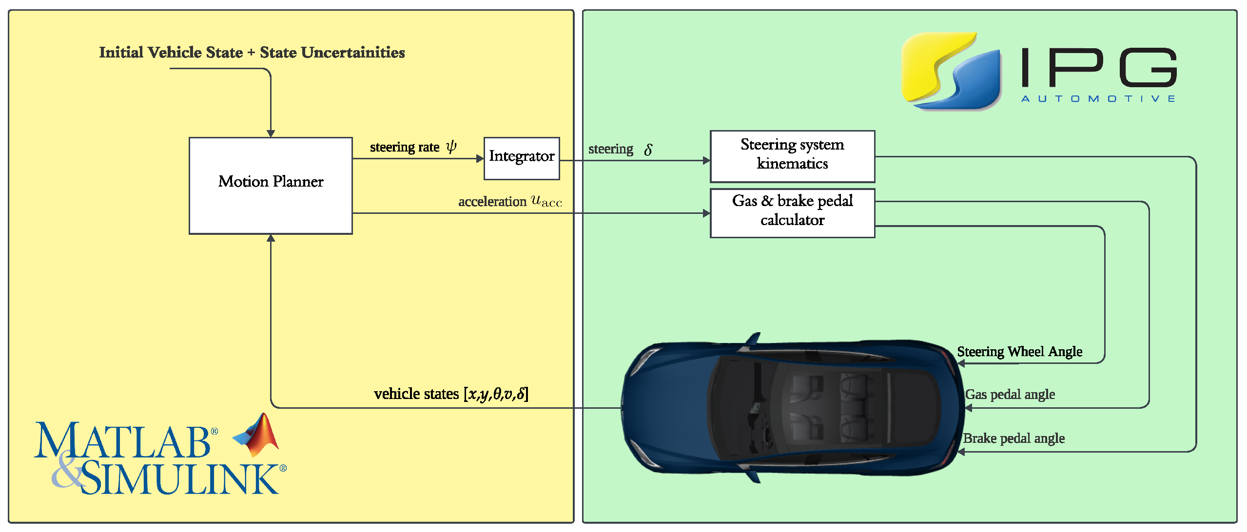
Futuretransp 04 00074 g002
Figure 3. Layout of feedback loop established between the developed motion planner and the high-fidelity simulation software.
Futuretransp 04 00074 g003
Figure 4. Uncertain cases (obstacle-avoidance set): robust for nominal case of 95 m relative distance and fewer failures as distance decreases.
Futuretransp 04 00074 g004
Figure 5. (a) Nominal cases for stationary OV case (obstacle-avoidance set): failures visible for high-speed scenarios but more robust under uncertainties. (b) Nominal cases for stationary OV case (path-following set): all pass but performs poorly under uncertainties in position information.
Futuretransp 04 00074 g005
Figure 6. Uncertain cases (path-following set): failures at all distances, failure modes are different from the first set of weights.
Futuretransp 04 00074 g006
Figure 7. obstacle-avoidance set simulation results: spread of scenarios with respect to starting position and heading.
Futuretransp 04 00074 g007
Figure 8. obstacle-avoidance set simulation results: scenario spread with respect to initial position and initial velocity.
Futuretransp 04 00074 g008
Figure 9. obstacle-avoidance set simulation results: scenario spread with respect to initial position and reference velocity.
Futuretransp 04 00074 g009
Figure 10. Nominal cases for moving-OV case under AV v ref of 17.5 m/s—all nominal cases pass successfully. Failures occur only in the presence of uncertainties, especially when y 0 , O V increases with a decrease in v 0 , OV .
Futuretransp 04 00074 g010
Figure 11. AV trajectory RMSE under moving-OV scenario for AV v ref of 17.5 m/s—failures only when y 0 , A V increases with decreases in v 0 , OV .
Futuretransp 04 00074 g011
Figure 12. Simulation results for the moving OV case under AV v ref of 17.5 m/s: (a) x 0 , AV vs. y 0 , AV vs. v 0 , OV most failures occur when y 0 , O V increases with decreases in v 0 , OV and x 0 , A V is at the edge of the 3 σ region; (b) x 0 , AV vs. y 0 , AV vs. heading ψ 0 , AV most failures occur when y 0 , O V increases with x 0 , A V at the right edge of the 3 σ region and with the initial heading angle to the right lane boundary.
Futuretransp 04 00074 g012
Figure 13. Nominal cases for moving-OV case under AV v ref of 25 m/s—all nominal cases pass successfully. Failures occur only in the presence of uncertainties, especially when y 0 , O V increases with a decrease in v 0 , OV .
Futuretransp 04 00074 g013
Figure 14. AV trajectory RMSE under moving-OV scenario for AV v ref of 25 m/s—failures only when y 0 , A V increases with decreases in v 0 , OV .
Futuretransp 04 00074 g014
Figure 15. Simulation results for the moving—OV case under AV v ref of 25 m/s: (a) x 0 , AV vs. y 0 , AV vs. v ref , AV —most failures occur when y 0 , A V increases with increases in v ref , AV and is invariant of x 0 , AV ; (b) x 0 , AV vs. y 0 , AV vs. heading ψ 0 , AV —most failures occur when y 0 , A V increases and is invariant of x 0 , AV and ψ 0 , AV .
Futuretransp 04 00074 g015
Figure 16. Nominal cases for safety-critical stopping scenario—failures occur when y 0 , AV increases with v ref , AV attributed to the shorter distance available for the AV to safely stop behind OV.
Futuretransp 04 00074 g016
Figure 17. AV trajectory RMSE under safety-critical scenario—failures occur when y 0 increases with failed case percentage increasing with increase in v ref , AV .
Futuretransp 04 00074 g017
Figure 18. Simulation results for the safety stop case: (a) x 0 , AV vs. y 0 , AV vs. v ref , AV —all the simulations corresponding to the failed nominal case failed too, i.e., the ones starting at 50 m and having a- velocity of 25 m/s; (b) x 0 , AV vs. y 0 , AV vs. heading ψ 0 , AV —the failures occur when the AV starts nearest to the OV, i.e., 50 m and is invariant of x 0 , AV and ψ 0 , AV .
Futuretransp 04 00074 g018
Table 1. Parameters and their ranges for the concrete and logical scenario description.
Parameter DescriptionSymbolUnitRangeUncertainty
AV x initial position x 0 , AV [m][0, 0] N ( x 0 , AV , 0 . 5 2 )
AV y initial position y 0 , AV [m][0, 50] N ( y 0 , AV , 1 . 5 2 )
OV initial position( x 0 , OV , y OV )[m][(0,100), (0,100)]
AV heading ψ 0 , AV [°][0, 0][−2, 2]
AV initial velocity v 0 , AV [m/s][0, 25]
AV reference position v ref , AV [m/s][10, 25]
OV velocity v 0 , OV [m/s][0, 24]
Table 2. Parameter set for static obstacle logical scenario.
ParameterUnitValueNominalUncertaintyUncertain
x 0 , AV [m][0]×1 N ( 0 , 0 . 5 2 )
y 0 , AV [m][5,20,35,50]×4 N ( y 0 , AV , 1 . 5 2 ) ×25
ψ 0 , AV (heading)[°][0]×1[−2,0,2]×3
v 0 , AV [m/s][0,3,6]×3
v ref , AV [m/s][10,17.5,25]×3
v 0 , OV [m/s][0]×1
Total Simulations 36×75 = 2700
Table 3. obstacle-avoidance set simulation results: heading v/s y 0 .
y 0 5203550
Heading
−2100%72%78%32%
0100%85%80%35%
2100%92%72%45%
Table 4. obstacle-avoidance set simulation results: v 0 v/s y 0 .
y 0 5203550
v 0
0100%85%75%36%
3100%83%73%40%
6100%80%82%37%
Table 5. obstacle-avoidance set simulation results: v ref v/s y 0 .
y 0 5203550
v ref
10100%88%88%50%
17.5100%61%45%52%
25100%100%97%11%
Table 6. Parameter set for the moving-obstacle logical scenario at v ref , AV = 17.5 m/s.
ParameterUnitValueNominalUncertaintyUncertain
x 0 , AV [m][0]×1 N ( 0 , 0 . 5 2 )
y 0 , AV [m][5,20,35,50]×4 N ( y 0 , AV , 1 . 5 2 ) ×25
ψ 0 , AV (heading)[°][0]×1[−2,0,2]×3
v 0 , AV [m/s] v ref , AV ×1
v ref , AV [m/s][17.5]×1
v 0 , OV [m/s][6,9,12,15]×4
Total Simulations 16×75 = 1200
Table 7. Simulation results for moving-OV case under AV v ref of 17.5 m/s— v obs vs. y 0 —number of failures increases when y 0 increases with a decrease in v obs attributed to the shorter distance available for the AV to react to the OV.
y 0 5203550
v obs
6100%100%76%65%
9100%100%100%81%
12100%100%100%100%
15100%100%100%99%
Table 8. Parameter set for moving-obstacle logical scenario at v ref , AV = 25 m/s.
ParameterUnitValueNominalUncertaintyUncertain
x 0 , AV [m][0]×1 N ( 0 , 0 . 5 2 )
y 0 , AV [m][5,20,35,50]×4 N ( y 0 , AV , 1 . 5 2 ) ×25
ψ 0 , AV (heading)[°][0]×1[−2,0,2]×3
v 0 , AV [m/s] v ref , AV ×1
v ref , AV [m/s][25]×1
v 0 , OV [m/s][6,12,18,24]×4
Total Simulations 16×75 = 1200
Table 9. Simulation results for moving-OV case under AV v ref of 25 m/s— v obs vs. y 0 —number of failures increases when y 0 increases with a decrease in v obs attributed to the shorter distance available for the AV to react to the OV.
y 0 5203550
v obs
6100%100%100%67%
12100%100%76%52%
18100%100%100%75%
24100%100%100%95%
Table 10. Parameter set for safety-critical scenario.
ParameterUnitValueNominalUncertaintyUncertain
x 0 , AV [m][0]×1 N ( 0 , 0 . 5 2 )
y 0 , AV [m][5,20,35,50]×4 N ( y 0 , AV , 1 . 5 2 ) ×25
ψ 0 , AV (heading)[°][0]×1[−2,0,2]×3
v 0 , AV [m/s] v 0 , AV
v ref , AV [m/s][10,17.5,25]×3
v 0 , OV [m/s][0]×1
Total Simulations 12×75 = 900
Table 11. Simulation results for safety-critical stopping scenario— v AV vs. y 0 —failures occur when y 0 , AV increases with v AV attributed to the shorter distance available for the AV to safely stop behind OV with more cases failing when v AV increases.
y 0 5203550
v AV
1099%100%100%83%
17.599%100%100%67%
2598%99%100%0%
Disclaimer/Publisher’s Note: The statements, opinions and data contained in all publications are solely those of the individual author(s) and contributor(s) and not of MDPI and/or the editor(s). MDPI and/or the editor(s) disclaim responsibility for any injury to people or property resulting from any ideas, methods, instructions or products referred to in the content.

