Abstract
Background: Quantum machine learning (QML) holds significant promise for advancing medical image classification. However, its practical application to large-scale, high-resolution datasets is constrained by the limited number of qubits and the inherent noise in current quantum hardware. Methods: In this study, we propose the Fused Quantum Dual-Backbone Network (FQDN), a novel hybrid architecture that integrates classical convolutional neural networks (CNNs) with quantum circuits. This design is optimized for the noisy intermediate-scale quantum (NISQ), enabling efficient computation despite hardware limitations. We evaluate FQDN on the task of gastrointestinal (GI) disease classification using wireless capsule endoscopy (WCE) images. Results: The proposed model achieves a substantial reduction in parameter complexity, with a 29.04% decrease in total parameters and a 94.44% reduction in trainable parameters, while outperforming its classical counterpart. FQDN achieves an accuracy of 95.80% on the validation set and 95.42% on the test set. Conclusions: These results demonstrate the potential of QML to enhance diagnostic accuracy in medical imaging.
1. Introduction
Artificial intelligence (AI) is currently playing a major role in the field of computer vision. It has helped so much in advancing medical imaging thanks to machine (ML) and deep learning (DL) [1,2]. Convolutional neural networks (CNNs) [3,4], transfer learning strategies [5], and transformers [6] have greatly advanced the domain, while ML and DL have shown impressive results. However, these approaches still suffer from numerous limitations. One of the biggest concerns is that these algorithms, when dealing with big datasets, require big computational resources, and sometimes it is hard to capture complex data patterns [7]. Quantum machine learning (QML) is a novel research era that can solve this problem [8,9].
QML combines the principles of quantum computing with machine learning principles. The purpose of this new era of research is to develop machine learning algorithms able to run on quantum computers [8]. These quantum machine algorithms will be efficient as they can solve the computational problem very easily [8]. Unlike classical computers that work using bits (0 and 1), quantum computers work using quantum bits (qubits). Quantum systems are more powerful as they can use quantum properties such as superposition and entanglement, which allow them to represent and process states simultaneously [10], explore a vast solution space in parallel, and accelerate learning tasks [11]. Currently, quantum systems still suffer from limited qubit counts and susceptibility to noise, which act as barriers to developing fully quantum algorithms. This period is referred to as the noisy intermediate-scale quantum (NISQ) era. However, recent research has shown that QML can be designed to operate within the constraints of NISQ hardware. A promising direction is the use of hybrid quantum–classical architectures [12,13,14], which combine classical learning frameworks with quantum components such as parametrized quantum circuits (PQCs) [15]. These architectures are usually built using CNNs or pre-trained models followed by variational quantum circuits [7,16]. For example, ref. [15] introduced two hybrid architectures for image classification. The first, is a hybrid quantum neural network with parallel quantum dense layers that uses CNNs for feature extraction and trains parallel quantum circuits for decision making. The second model, is called HQNN-Quanv, which has a quanvolutional layer that performs quantum convolution operations and reduces input dimensionality while maintaining important features. Following the same direction, ref. [17] proposed quantum neural networks (QNNs), that use quantum convolutional layers in CNNs, allowing the use of quantum filters for localized feature transformation and improved accuracy. In another notable contribution, ref. [18] evaluated the impact of quantum layers on classical architectures like VGG-16, ResNet-18, and AlexNet for histopathological cancer image classification. Their study demonstrated that augmenting these networks with variational quantum circuits could improve performance, showing the power of QML for medical applications.
In this work, we present a new hybrid QML model that uses both classical learning techniques with PQCs. Our approach combines model fusion with quantum processing to construct an efficient architecture that reduces the number of parameters while improving classification accuracy compared to purely classical models. The key contributions of this study are as follows:
- We propose a hybrid quantum–classical framework that effectively combines classical machine learning with quantum computational components.
- We use quantum circuits to improve the model’s ability to detect complex patterns in medical imaging data.
- We demonstrate that our model achieves superior classification performance with significantly fewer trainable parameters than its classical counterparts.
The rest of this paper is organized as follows: Section 2 reviews existing deep learning methods for detecting gastrointestinal diseases using wireless capsule endoscopy (WCE) images. Section 3 explains the variational quantum circuit. Section 4 describes the proposed method and provides a detailed explanation of the FQDN architecture. Section 5 presents the experimental setup, results, and analysis. Finally, Section 6 gives conclusions and discusses future directions.
2. Literature Review
This section provides a review of existing classical approaches based on the techniques used. We divided the review into two main parts based on the existing number of papers and the techniques used: convolutional neural networks and Vision Transformer-based methods; followed by transfer learning-based methods. To date, for gastrointestinal (GI) diseases, there exist no quantum machine learning approaches to be included in this section. For this reason, we restrict our research to classical machine learning and deep learning approaches.
2.1. CNN- and Vision Transformer (ViT)-Based Methods
Medical image classification is a challenge of paramount importance in healthcare. Following deep learning approaches, many research studies have succeeded in classification of gastrointestinal (GI) diseases. Convolutional neural networks (CNNs) are highly used due to their capacity in feature extraction and classification in the medical imaging domain. Ref. [19] proposed a CNN ensemble framework that demonstrated improved performance in detecting bleeding symptoms in capsule endoscopy (CE) images for a binary classification problem, achieving 95% accuracy on a public dataset and 93% accuracy on a real-world validation dataset. However, the efficacy of this approach relies greatly on the quality of input images. Variability in endoscopic image quality in real-world settings may degrade model performance. Furthermore, the reliance on handcrafted feature engineering introduces additional complexity. Alternatively, ref. [20] conducted a benchmark comparison of four models: CNN, CNN-RNN, CNN-BiLSTM, and CNN-GRU. Their findings indicate that CNNs followed by a Gated Recurrent Unit (GRU) give the highest accuracy (99%) in classifying WCE images into normal and bleeding categories within the test dataset. While this approach demonstrated efficacy in a binary classification scenario, its performance in multi-class problems is worth further investigation.
Recent research has explored the integration of Vision Transformers (ViTs) to improve classification accuracy. ViTs are capable of capturing long-range dependencies and global correlations within images, making them suitable for medical image classification tasks. Ref. [21] utilized a transformer-based model for classifying images extracted from endoscopic capsule videos, achieving 99.70% accuracy, 99.64% precision, 99.86% sensitivity, and 99.54% F1-score on the Kvasir Capsule dataset. This study demonstrates the potential of ViTs for improved classification accuracy. Another study [22] also focused on Vision Transformers, integrating a residual block with a ViT backbone and a spatial attention mechanism to effectively process both local and global image features. Evaluation on publicly available datasets, including Kvasir and ETIS-Larib, revealed accuracies of 96.4% in binary classification and 99.7% in multi-class classification. Ref. [23] proposed a Vision Transformer with shifted windows for gastrointestinal endoscopy image classification, achieving 95.42% accuracy on the Kvasir v2 dataset and 86.81% accuracy on the HyperKvasir dataset. Ref. [24] investigated an attention mechanism within a convolutional neural network for local feature extraction, achieving 97% accuracy on the public Kvasir Capsule Endoscopy dataset. However, for medical image datasets, the application of pre-trained models, known as transfer learning, remains one of the best approaches to follow for achieving accurate classification.
2.2. Transfer Learning-Based Methods
Transfer learning involves the application of pre-trained models, developed initially on large datasets such as ImageNet [25], to specific tasks. This technique transfers knowledge gained by the model to address a particular problem. Ref. [26] utilized pre-trained models, including AlexNet, VGG16, VGG19, ResNet50, and ResNet101, fine-tuning them on a colonoscopy image dataset comprising four classes: Normal, inflammation, polyps, and cancer. The combination of these models with data augmentation techniques resulted in improved classification accuracy, with ResNet50 achieving 94.98% accuracy. This represents an improvement over traditional models trained from scratch. However, this study primarily focused on accuracy, with limited consideration of the number of parameters. The use of a relatively small training dataset with models possessing a large number of parameters, such as ResNet50 with approximately 25 million parameters, may increase the risk of overfitting. Ref. [27] utilized AlexNet CNN for feature extraction, followed by fine-tuning on a capsule endoscopy (CE) image dataset to identify differences between bleeding and non-bleeding frames. Furthermore, they integrated a SegNet-based deep learning model for a pixel-wise bleeding zone, achieving an F1-score of 98.49% for bleeding frame detection and a global accuracy of 94.43% for bleeding zone identification. Ref. [28] also investigated transfer learning for classifying abnormalities in a small, unbalanced wireless endoscopy image (WCE) dataset. They evaluated the performance of EfficientNet, ResNet50, and Xception. ResNet50 reached the highest performance, with 97% precision, 99% recall, and an F1-score of 98%. However, given the unbalanced nature of the dataset, further benchmarking using additional transfer learning models could have been conducted. Ref. [29] explored the efficacy of transfer learning models in classifying gastrointestinal (GI) tract anomalies, retraining VGG16, ResNet, MobilNet, Inception-v3, and Xception using the Kvasir dataset. VGG16 and Xception achieved top performances of 98.3% and 98.2% accuracy, respectively. Ref. [30] applied transfer learning, but further they used explainable AI methods, such as Grad-weighted Class Activation Mapping (Grad-CAM) and its variants (Grad-CAM++, Hires-CAM, Score-CAM) to generate heatmaps, highlighting the regions contributing most to model predictions. The models used included DenseNet201, MobileNetV2, ResNet152, ResNet18, and VGG16, with ResNet152 achieving the highest classification accuracy (98.28%) and validation accuracy (93.46%). This research contributes to improving the transparency and reliability of deep learning models in medical diagnostics through the application of explainable AI techniques. Ref. [31] utilized model fusion with feature selection to improve model performance, achieving 96.43% accuracy. Their approach used ResNet152 and ResNet50 with Ant Colony Optimization (ACO) for feature selection after fusion to eliminate redundant features. However, this approach relies heavily on feature engineering, utilizing Mask R-CNN for gastrointestinal disease localization. Also, the total and trainable parameters of their model were not specified. Ref. [32] applied transfer learning on the Kvasir dataset, specifically using VGG19 and ResNet50. ResNet50 achieved the highest validation accuracy, 96.81%; recall, 95.28%, precision, 95%; and F1-score, 94.85%. Similarly, ref. [33] used an ensemble transfer learning approach, proposing a weighted average ensemble model for GI-tract disease classification, achieving 95% accuracy on the Kvasir v2 dataset. Ref. [34] focused on pre-trained models, specifically AlexNet, DenseNet201, InceptionV3, and ResNet101, on the HyperKvasir dataset, achieving 97.11% accuracy with DenseNet201.
3. Variational Quantum Circuit
The variational quantum circuit (VQC) is a quantum computing model. The core idea of it is inspired by neural networks in deep learning. It has been used in many studies including [7,15,35,36]. A VQC can have multiple layers of quantum gates, including single-qubit rotation gates, whose angles are parameterized by classical values optimized during training; and entangling layers, often composed of CNOT (Controlled-NOT) gates, that introduce quantum correlations (entanglement) among qubits to enable complex computations. Before the application of parameterized layers, a critical preprocessing step, referred to as data embedding, should be performed to encode classical data into quantum data, which is then input into the VQC for computational processing.
3.1. Data Embedding
In machine learning, when we have categorical data we transform this data to numerical using embedding techniques, because only the numbers are understood. Similarly, in quantum circuits we need to transform classical data into quantum data because quantum circuits can only operate on quantum states. Specifically, a classical feature vector is encoded into the state of qubits, which enables subsequent quantum operations.
- (a)
- Initial quantum state: The quantum system is initialized in the state , representing qubits, each in the state . Here, the symbol ⊗ denotes the tensor product, a mathematical operation used to combine the states of individual qubits into a single multi-qubit state. For instance, if , the initial state is .
- (b)
- Embedding technique: Several techniques exist for embedding classical data into quantum states: (1) amplitude encoding [37], which utilizes the amplitudes of the quantum state to represent data; (2) basis encoding [38], which maps data to specific computational basis states; (3) Hamiltonian-based embeddings [39], which leverage problem-specific Hamiltonians, and a common embedding technique called angle embedding [40], where classical features are encoded into the rotation angles of single-qubit gates ( or or ), providing a straightforward and efficient data-loading mechanism. Due to its minimal number of qubits, hardware efficiency, and gate requirements, we used angle embedding as the embedding technique.
To encode classical data x into the quantum system, a unitary operation is applied. This operation transforms the initial state into a new quantum state , effectively embedding the classical data into the quantum system:
We denote this embedding operation by
3.2. Parameterized Quantum Layer
Once the data is embedded, the VQC applies one or more quantum layers to process the embedded state. A generic quantum layer is defined by a trainable unitary operation, where w represents the weights. Acting on an input state , this layer’s outputs are
3.3. Measurement
After data passes through the parameterized quantum layers, we obtain a final quantum state . This quantum state contains the processed information, but we need to extract classical results from it through measurement.
In quantum mechanics, measurement is fundamentally different from classical observation. When we measure a quantum system, we force it to collapse from a superposition state to one of its basis states. This process follows the following principles.
First, we have the quantum measurement process, in which the measurement projects the quantum state into one of the computational basis states or for a single qubit. This projection is probabilistic, with probabilities determined by the quantum state. For a state , the probability of measuring is and the probability of measuring is . second, Pauli measurements, which are the most common measurement approach, use Pauli operators, particularly the Pauli-Z operator (denoted as for the i-th qubit). This operator is represented by the matrix
When applied to a qubit, the Pauli-Z operator determines whether the qubit is more likely to be in the state (eigenvalue ) or the state (eigenvalue ).
Third, we have expectation values: Instead of single-shot measurements that give binary outcomes, quantum algorithms typically work with expectation values. The expectation value of the Pauli-Z operator for the i-th qubit is calculated as
This quantity represents the average result we would obtain if we performed many measurements on identical copies of the state .
The entire measurement process transforms the quantum state into classical information that can be further processed or analyzed:
This mapping completes the quantum–classical hybrid approach of variational quantum circuits, allowing us to use quantum computations for practical applications.
3.4. Overall Structure of the VQC
A variational quantum circuit can be seen as being composed of three functions:
- Embedding , which maps classical data to a quantum state.
- Parameterized layers , which perform trainable transformations on that quantum state.
- Measurement , which recovers a classical result .
Symbolically,
Here,
- : The overall VQC, taking a classical input and returning a classical output .
- ∘: Denotes function composition.
4. Proposed Method
This work proposes the Fused Quantum Dual-Backbone Network (FQDN) for the classification of gastrointestinal (GI) diseases (see Figure 1). The FQDN integrates MobileNetV2 and EfficientNetB0 for feature extraction. The classifier layers of both networks are replaced with identity mappings, preserving only the feature extraction pipeline while freezing their parameters to reduce training complexity. The extracted features from each network are processed through separate quantum layers, and the quantum-enhanced features are subsequently fused and passed to a classifier for final classification.
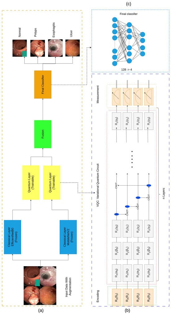
Figure 1.
The architecture of the proposed model. (a) shows the Fused Quantum Dual-Backbone Network (FQDN). (b) shows the quantum layer that contains three main parts: the data encoding part that transforms classical data into quantum data using the angle embedding technique, then the variational quantum circuit to perform quantum computations on the data, and the final part is called measurements. The quantum-enhanced features are then fused and passed through the fully connected network (FCN) for the classification part, as represented in (c).
4.1. Feature Extraction with Pretrained Models
Following standard transfer learning practices [41], we used the MobileNetV2 and EfficientNetB0 models that were originally trained on ImageNet, a large dataset covering diverse objects and images [25]. We took advantage of their built-in feature extraction capabilities for new tasks, which may involve a different domain. As shown in Figure 1a, all layers in these pre-trained models were frozen (i.e., no weight updates occurred). Moreover, we removed the final classification layer in each model and replaced it with an identity mapping. As a result, these networks now output high-dimensional feature vectors, rather than class probability distributions, and thus serve purely as static feature extractors [7]. In the experimental setup, the final classification layer of each pre-trained model was substituted with an identity mapping. It is noted that alternative model combinations were evaluated; however, the proposed combination gave the optimal fusion performance. Substituting with other models rather than MobileNetV2 and EfficientNetB0 did not result in improved performance, even with a higher number of parameters.
4.1.1. MobileNetV2
MobileNetV2, introduced by Sandler et al. (2018) [42], is a deep learning model designed to balance accuracy with computational efficiency. It achieves this using depthwise separable convolution and inverted residuals with linear bottlenecks.
Depthwise separable convolutions: Traditional convolution layers apply each filter across all input channels, which can be computationally expensive. MobileNetV2 reduces this cost by breaking this operation into two parts:
- Depthwise convolution: This applies a single convolutional filter to each input channel individually, rather than all channels at once. Mathematically, for an input feature map , the depthwise convolution is defined aswhere represents the depthwise convolutional kernels, and denote the spatial offsets for the height and width dimensions, respectively, K is the size of the convolutional kernel, h and w are the spatial indices for height and width, and c indexes the input channels. This operation ensures that each input channel is convolved independently to keep the number of channels in the output feature map.
- Pointwise convolution: Pointwise convolution utilizes convolutions to combine the outputs of the depthwise convolution across channels. For an intermediate feature map , the pointwise convolution is defined aswhere the pointwise convolutional kernels are expressed as and there are output channels of the pointwise convolution, h and w are spatial indices for the height and width, c represents the index of the input channels, and represents the index of the output channels. Pointwise convolution combines the information across channels, which allows the network to learn more features by merging the spatial data offered by depthwise convolution.The combination of these two operations forms the backbone of efficient architectures. By separating spatial and channel-wise processing, these operations reduce the number of parameters and computational costs while preserving the ability to capture rich feature representations [42]. The final feature map is given bywhere refers to the final feature map after performing pointwise convolution on the output of depthwise convolution on the input .
- Inverted residuals with linear bottlenecks: Another main feature in MobileNetV2 is the inverted residual block, which reverses the traditional residual block structure. Instead of reducing and expanding the feature dimensions, it first expands the number of channels, performs convolutions, and then projects the result back to lower-dimensional space. Each block consists of the following:
- -
- Expansion: The number of channels in the input feature map is increased.
- -
- Depthwise convolution: A depthwise convolution is applied to the expanded feature map, further increasing the spatial feature dimensionality within each channel.
- -
- Projection: A pointwise convolution is utilized to reduce the number of channels back to the original input dimension.
4.1.2. EfficientNetB0
The EfficientNet architecture [43] uses a strategy called compound scaling to expand the depth, width, and input resolution of a neural network in a balanced way. This approach improves model accuracy without greatly increasing computational demands. The idea is to manage these three dimensions with a single parameter, ensuring the network grows proportionally in all relevant directions.
According to [44,45], compound scaling relies on three factors, , , and , which adjust the network’s depth, width, and resolution, respectively. Each factor is given by a single overall scaling parameter :
where
- d controls the depth of the network;
- w controls the width of the network, meaning the number of channels per layer;
- r controls the resolution of the image;
- is a constant that the user chooses, which decides the scaling of the whole network.
These scaling factors are chosen so that
This formula ensures that as the model is scaled up, no single dimension dominates resource usage, which leads to better accuracy with minimal increase in cost.
4.2. Quantum Circuit Integration
In the proposed hybrid classical–quantum architecture, feature extraction is performed using two pre-trained classical models. The result is high-dimensional feature vectors. These vectors are subsequently processed by a quantum layer consisting of a four-qubit quantum circuit. This design choice is to take into consideration the limitations of the NISQ era, where increasing qubit counts in hybrid algorithms can negatively impact performance. Each feature vector is encoded and processed independently within its corresponding quantum layer. The data encoding process involves the following stages.
4.2.1. Linear Transformation
Following feature extraction, the high-dimensional feature vectors are subjected to dimensionality reduction to match the input dimension of the four-qubit quantum circuit. This reduction is achieved via a linear transformation, mathematically defined as
where
- : Original input feature vector extracted from MobileNetV2 and EfficientNetB0;
- : Weight matrix of the linear layer, transforming the input from n dimensions to 4 dimensions;
- : Bias vector of the linear layer;
- : Reduced feature vector for quantum processing.
This linear transformation ensures that the high-dimensional features are condensed into a form compatible with the quantum circuit, reducing computational complexity while keeping essential information.
4.2.2. Angle Embedding
The reduced classical feature vector is encoded into quantum states using angle embedding. As mentioned above, this method maps each classical feature to a rotation angle applied to the corresponding qubit. The initial state of the quantum system is , meaning all four qubits are initialized to the ground state . The angle embedding process transforms this initial state into a new quantum state as follows:
where is the rotational X gate that rotates the qubit around the X-axis by angle .
The rotational X gate is mathematically represented as
4.2.3. Variational Quantum Circuit
The variational quantum circuit (VQC), as represented in Figure 1b, comprises a combination of parameterized single-qubit rotation gates and two-qubit entangling gates, structured to capture complex feature interactions and correlations. For the parameterized rotation gates, each qubit within the VQC has a series of adjustable rotation gates, specifically , , and gates. These gates are controlled by trainable parameters , , and , which are optimized during the training process to manipulate the quantum states based on the input data:
where
- : Sequence of rotation operations applied to each qubit;
- , , : Trainable parameters for rotations around the X, Y, and Z axes, respectively.
The rotation gates are mathematically represented as
These rotation gates manipulate the quantum states of the qubits, enabling the VQC to model complex, non-linear transformations. These transformations are essential for capturing feature interactions in the data.
To introduce quantum entanglement, a phenomenon where qubits become interdependent regardless of their spatial separation, we use Controlled-NOT (CNOT) gates between pairs of qubits. The CNOT gate is a two-qubit gate that flips the state of the target qubit () if and only if the control qubit () is in the state . Mathematically, the action of the CNOT gate can be described as
where is the state of the target qubit and ⊕ denotes addition modulo 2. The overall entanglement operation in the circuit is defined as
This process ensures that each qubit is correlated with its neighbors, which helps for the propagation of quantum information across the whole circuit.
4.2.4. Overall VQC Operation
Combining the rotation and entangling operations, the VQC is mathematically represented as
where
- : Trainable parameters of the VQC.
- : Denotes the function of composition.
4.3. Measurement
The final stage of the quantum circuit is measurement, where the quantum states are projected back into the classical domain. This process involves evaluating the Pauli-Z operators for each qubit, resulting in a classical vector :
where is the expectation value of the Pauli-Z operator for the qubit, and the Pauli-Z operator (Z) is defined as
It has eigenvalues of (corresponding to the state ) and (corresponding to the state ).
The expectation value is computed as
where is the quantum state after data encoding and transformations (e.g., rotation gates and entanglement), is the Pauli-Z operator acting on the qubit, and is the bra vector (the conjugate transpose of ).
The expectation value represents the average outcome of measuring the qubit in the computational basis ( and ). The measurement process is repeated multiple times to estimate accurately. The resulting classical vector encapsulates the quantum information in a form suitable for classical post-processing.
4.4. Optimization
The optimization process involves adjusting the trainable parameters of the VQC, specifically, the rotation angles , , and , to minimize a loss function. The loss function measures how well the model’s predictions match the true labels in the training dataset. The optimization is performed using the AdamW optimizer.
4.4.1. Gradient Approximation
To update the parameters, we need to compute the gradient of the loss function with respect to each trainable quantum parameter . In quantum circuits, this is achieved using the parameter-shift rule, which allows for exact gradient computation of expectation values with respect to circuit parameters. The gradient of the loss function with respect to a parameter is given by
where
- : The loss evaluated after shifting the parameter by ;
- : The loss evaluated after shifting the parameter by .
4.4.2. Parameter Update Rule
Once the gradient is computed, the parameters are updated using the AdamW optimizer [46]. AdamW is an extension of Adam that decouples weight decay from the gradient-based updates. The update rule for a parameter at iteration t is
where
- : Parameter vector at iteration t;
- : The learning rate; a hyperparameter that determines the step size for the update;
- : The gradient of the loss function for .
4.4.3. Loss Function
For classification, the cross-entropy loss function is used:
where
- n: Number of classes;
- : The true probability distribution;
- : The predicted probability distribution.
The cross-entropy loss penalizes incorrect classifications, ensuring the model’s predictions align with the true labels.
5. Experiments and Results
In this section we describe the dataset used. Then, we detail the network setup and configuration. Finally, we present and analyze the experimental results obtained.
5.1. Dataset
5.1.1. Dataset Details
The dataset utilized in this study is the WCE Curated Disease Dataset [47,48]. This dataset contains a collection of wireless capsule endoscopy (WCE) images specifically related to colonic diseases. This dataset was constructed for research purposes by integrating image data from two gastrointestinal image datasets: the Kvasir dataset [49] and the ETIS-Larib-Polyp DB dataset [50].
The dataset contains four classes as shown in Figure 2:
- Normal: Represents healthy intestinal tissue with normal color and surface texture [48].
- Polyps: Small growths on the colon lining, appearing individually or in groups, with distinct color and texture differences from surrounding tissue. While most polyps are benign and cause no symptoms, some types may develop into colorectal cancer [48].
- Esophagitis: Inflammation of the esophagus. Common symptoms include heartburn, pain, and sore throat. Without treatment, complications can include ulcers and bleeding, which may cause painful swallowing [48].
- Ulcers: A condition affecting the large intestine’s lining, causing inflammation ranging from mild to severe. Ulcerative areas often show a white coating where the body is attempting to heal damaged tissue [48]. Patients with this condition are at higher risk of cancer compared to other people.

Figure 2.
Raw samples and corresponding classes.
Our dataset contains 6000 RGB images in total. A structured distribution was implemented to split the dataset. A total of 3200 images (53.3%) were allocated for training, 2000 images (33.3%) for validation, and 800 images (13.3%) for testing. The dataset has equal distribution across all four diagnostic categories, with 800 samples per class for training, 500 samples per class for validation, and 200 samples per class for testing. The original images have dimensional heterogeneity due to their diverse origins. To address this, all images were standardized to a resolution of 224 × 224 pixels before being fed into the neural network architecture. This basically ensures that the feature extraction is consistent while preserving the essential diagnostic characteristics of the endoscopic imagery.
5.1.2. Data Augmentation and Normalization
During the training phase, we applied several data augmentation techniques to increase the diversity of our data and help the model generalize better. These techniques included random resized cropping, horizontal and vertical flipping, random rotations, and color jittering. Additionally, we normalized the images using mean values [0.485, 0.456, 0.406] and standard deviations [0.229, 0.224, 0.225], which are commonly used for models pre-trained on ImageNet. This normalization ensures that all images have similar brightness and contrast, making the training process more efficient. For the validation and testing sets, we resized the images to 256 × 256 pixels and then took a center crop to 224 × 224 pixels, without applying any augmentation.
Table 1 summarizes the data augmentation and normalization techniques used.

Table 1.
Data augmentation techniques.
5.2. Network Setup and Training
For the quantum machine learning (QML) experiment, we used Pennylane [51], the open-source framework developed by Xanadu. There exist other frameworks such as Qiskit and tensorflow-quantum, but after experimentation we found that Pennylane was more suitable as it could be integrated and used with pytorch. The FQDN was trained over 100 epochs with early stopping set to 30 epochs to prevent overfitting and reduce unnecessary computation once the validation performance stopped improving. For the classical machine learning components, we employed pytorch, using the AdamW optimizer [46] with a learning rate of . The batch size was set to 32.
5.3. Diagnostic Metrics
For our task of medical image classification, we performed evaluation using accuracy, precision, recall, and F1-score [52,53]. The following equations define the metrics used:
5.4. Results and Discussion
To evaluate the performance of the FQDN, we first evaluated the performance of each individual component. We trained the MobileNetV2 and EfficientNetB0 models on our dataset to establish baseline metrics. Then, we compared the FQDN and its classical counterpart, which combines both backbones without quantum layers. To evaluate our model further, we conducted a comparison with previous studies that utilized the same dataset. Following these performance comparisons, we applied SHAP (Shapley Additive Explanations) to understand the predictions of our model, and to highlight the regions that most influenced the decision-making process of the FQDN.
5.4.1. Number of Parameters
The Fused Quantum Dual-Backbone Network (FQDN) achieves a 29% reduction in total parameters (6,385,204 vs. 8,998,412) and a 94% decrease in trainable parameters (153,784 vs. 2,766,992) compared to the classical model, as illustrated in Figure 3. Despite this reduction in parameter count, the FQDN achieves superior performance metrics compared to its classical counterpart, as will be demonstrated. This enhanced performance highlights the efficiency and effectiveness of the FQDN in classifying gastrointestinal (GI) diseases.
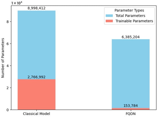
Figure 3.
Number of parameters: FQDN vs. classical version.
5.4.2. Performance Analysis
To evaluate the contribution of the quantum layer, we conducted a component-wise analysis. First, we trained the individual backbones on the dataset separately; MobileNetV2 with 4.34 M parameters and EfficientNetB0 with 2.55 M parameters. Training of MobileNetV2 stopped at epoch 49 due to early stopping, achieving 91.37% accuracy on the test set, while EfficientNetB0 stopped at epoch 59 for the same reason to prevent overfitting, and demonstrated superior performance at 94.13% (see Figure 4 and Table 2). The classical fusion model, combining both backbones without quantum enhancement, achieved 94.67% accuracy using 8.99 M total parameters (2.77 M trainable). While this represents a 0.54% improvement over the best individual backbone, it required significantly more parameters. In contrast, the FQDN achieved 95.42% accuracy with 6.39 M total parameters but only 153,784 trainable parameters.
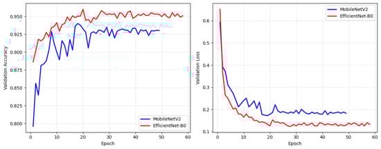
Figure 4.
Validation accuracy and validation loss curves for MobileNetV2 and EfficientNetB0.
Table 2.
Comprehensive performance comparison of all models.
Figure 5 shows the smooth convergence of the FQDN, reaching its peak performance of 96.30% validation accuracy by epoch 20, with minimal fluctuation throughout the remaining 60 epochs. The validation accuracy curve shows a standard deviation of less than 0.5% after convergence, which indicates stability in the training. On the other hand, the classical model shows more volatile behavior, with validation accuracy oscillating between 94.5% and 95.7%. The training time of the FQDN (48.72 s per epoch, totaling 81.20 min for 100 epochs) is higher than that of the classical model (44.42 s per epoch, totaling 74.03 min for 100 epochs) (see Figure 5e,f), primarily due to the additional computational cost of simulating quantum circuits during training.
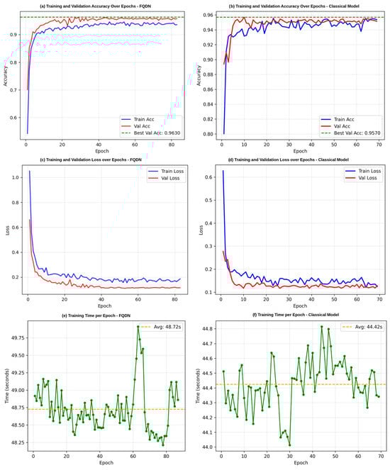
Figure 5.
Training and validation performance comparison between the FQDN model and the classical model. (a,b) Training and validation accuracy by epoch for the FQDN model and classical model, respectively. (c,d) Training and validation loss by epoch for the two models. (e,f) Training time per epoch.
Examining the results presented in Table 3, our Fused Quantum Dual-Backbone Network (FQDN) demonstrates higher performance compared to its classical model across all evaluation metrics. The FQDN achieved an overall accuracy of 95%, surpassing the classical model, which achieved a lower accuracy of 94%. This improvement becomes more meaningful when we analyze the performance across specific diagnostic categories. For normal tissue, the FQDN reached 97% precision and 100% recall, resulting in an impressive F1-score of 99%. This indicates that the FQDN was able to correctly classify healthy tissue samples without false positives. In the challenging category of ulcerative colitis, our FQDN showed more balanced detection capabilities, with 93% precision, 91% recall, and an F1-score of 92%. While the classical model achieved higher precision of 97%, its lower recall of 87% resulted in an inferior F1-score of 91%. This difference is clinically significant, as the FQDN’s higher recall means fewer missed cases of this serious condition. For polyps, the FQDN again outperformed the classical model, with precision and recall values of 91% and 92%, respectively, compared to 89% and 93%. Both models performed well in identifying esophagitis, with the FQDN achieving 100% precision and 99% recall and the classical model achieving 100% in both precision and recall. These results show that integrating quantum circuits into neural network architectures improves diagnostic performance for gastrointestinal conditions, particularly for challenging categories, where detection accuracy impacts clinical decision making.
Table 3.
Comparison of performance metrics between FQDN and classical model.
Additionally, the validation set confusion matrices show important performance differences between the Fused Quantum Dual-Backbone Network (FQDN) and the classical model. In the FQDN confusion matrix (Figure 6a), we see a perfect classification of normal cases, with all 500 samples correctly identified. For ulcerative colitis, 457 out of 500 cases were correctly classified, with only 2 misclassified as normal, 39 as polyps, and 2 as esophagitis. The polyp category shows 461 correct classifications out of 500 samples, with 8 misclassified as normal and 31 as ulcerative colitis. Esophagitis demonstrates excellent performance, with 498 correct classifications and only 2 samples misclassified as ulcerative colitis. The classical model confusion matrix (Figure 6c) also shows perfect classification of normal cases, with all 500 samples correctly identified. However, its performance differs notably in other categories. For ulcerative colitis, 429 out of 500 cases are correctly classified, with 14 misclassified as normal, 54 as polyps, and 3 as esophagitis. The polyp category shows 459 correct classifications out of 500 samples, with 26 misclassified as normal and 15 as ulcerative colitis. Esophagitis achieves a very good classification, with 499 samples correctly identified and only 1 misclassified as normal. The ROC curves presented in Figure 6b,d explain these performance differences. For class 0 (normal) and class 3 (esophagitis), we see that both models demonstrate excellent performance, with curves rapidly approaching a 100% true positive rate with minimal false positives, confirming the perfect classification seen in the validation confusion matrices. For classes 1 (ulcerative colitis) and 2 (polyps), the FQDN’s ROC curve rises more and remains closer to the ideal upper-left corner compared to the classical model’s curve. This shows that the FQDN is better in terms of classifying ulcers and polyps, demonstrating the efficacy of the FQDN at correctly identifying significant categories where clinical decision making is most sensitive (see Figure 7). We also used cross-validation to validate the performance of the FQDN and to ensure the consistency of our approach. For this we used 5-fold cross-validation (see Figure 8a,b). The FQDN consistently performed well across all folds, with a mean accuracy of 95.37 ± 0.71% (95% CI: [94.75%, 95.99%]). the confidence interval and the standard deviation confirm that the quantum enhancement provides stable improvements rather than benefiting from favorable data splits. To evaluate the generalization capability of our model we conducted an external validation using the Kvasir dataset [49], a collection of gastrointestinal (GI) endoscopy images. The original Kvasir dataset contains multiple endoscopic findings; however, to ensure the consistent evaluation, we kept only the four categories matching our classes in the training. Other categories like dyed-lifted-polyps and dyed-resection margins were excluded. The model was evaluated on 2300 images with 800 normal cases and 500 images for each of the other classes. The FQDN achieved 94.48% accuracy on this dataset without any fine-tuning or adaption, showing only a 0.94% decrease from the internal test set. Looking at Figure 8c, we see that the model maintained strong per-class performance: Normal tissue classification achieved 99.75% accuracy, esophagitis 97.20%, ulcerative colitis 90.40%, and polyps 87.40%. The confusion matrix (see Figure 8d) shows that normal and esophagitis were the classes with the highest scores, with nearly perfect classification on the normal class. However, the most challenging discrimination remains between ulcers and polyps. The model correctly identified 452 of 500 ulcerative colitis cases (90.40% accuracy) but showed some confusion with polyps (41 cases). Similarly, polyp detection achieved 87.40% accuracy, with 52 cases misclassified as ulcerative colitis. For explainable AI, we employed Shapley Additive Explanations (SHAP) to analyze the FQDN model’s decision-making process (see Figure 9). The SHAP analysis shows that the FQDN has learned clinically relevant features rather than spurious correlations. For example, for the polyps class, we see the most localized SHAP patterns, with high positive values, concentrated directly on the polypoid lesions, while the surrounding normal mucosa shows negative SHAP values, which demonstrates the model’s ability to distinguish between lesion and background tissue.
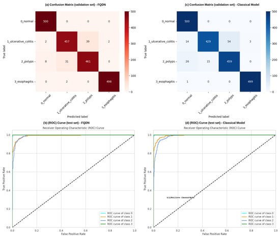
Figure 6.
Performance analysis and comparison between the FQDN and its classical counterpart. (a,b) show the confusion matrix and the ROC curve for the FQDN, respectively, while (c,d) show the confusion matrix and the ROC curve of the classical model without quantum layers, respectively.
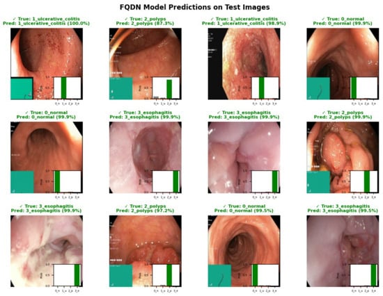
Figure 7.
Representative predictions of the FQDN model on test images, with ground truth labels, predicted labels, and associated probability distributions.
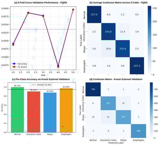
Figure 8.
Performance validation of the FQDN model. (a) shows the results of the 5-fold cross-validation, showing accuracy and F1-score across individual folds, with an overall mean accuracy of 95.37%. (b) Average confusion matrix across all 5 folds, while (c,d) show the per-accuracy class on the Kvasir dataset and the confusion matrix, respectively.
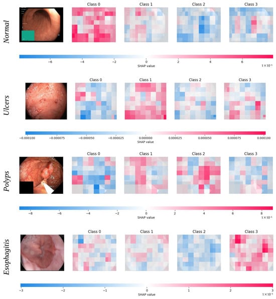
Figure 9.
SHAP-based interpretability analysis of the FQDN model for representative samples from each disease category. For each image, SHAP value heatmaps for all four output classes (0—normal, 1—ulcers, 2—polyps, 3—esophagitis) are shown. Red regions indicate image areas with a positive contribution to the predicted probability of the corresponding class, while blue regions indicate a negative contribution, with color intensity reflecting the magnitude of influence.
For further evaluation, a quantitative comparison was performed between the Fused Quantum Dual-Backbone Network (FQDN) model and recent methodologies applied to the WCE Curated Colon Disease Dataset, as detailed in Table 4. The FQDN model shows a better performance compared to other approaches, offering both higher accuracy and practical efficiency. In [54] we see that the Vision Transformer (ViT) holds slightly higher accuracy (95.63%), but it comes with significant computational demands. ViTs rely on patch-wise processing and self-attention mechanisms, which mean they require more computational resources and are harder to deploy. In contrast, the FQDN achieves nearly the same performance and accuracy (95.42%) but with only 6.38 million parameters, far fewer than ViT or DenseNet201 [54], which has 66.5 million. This makes the FQDN a far more practical option for real-world healthcare environments, where hardware limitations are a common challenge. On the other hand, traditional convolutional networks like VGG16 and InceptionV3 [55], despite achieving good results (94%), are based on fixed hierarchical features. These static patterns often fall short when it comes to capturing the complex irregular nature of gastrointestinal lesions. The FQDN handles these limitations by using dynamic, multi-scale feature fusion and quantum-enhanced representation learning. Also, the FQDN uses only 153,412 trainable parameters, while VGG16 uses 529,412 and InceptionV3 uses 21.8 million, making it more efficient in terms of computational resources. FQDN’s balanced performance, achieving 95.42% precision and 95.45% recall, shows its reliability in real-world applications.
Table 4.
Comparative analysis of the proposed model against recent works on the WCE Curated Colon Disease Dataset.
6. Conclusions and Future Perspectives
In this paper, we presented the Fused Quantum Dual-Backbone Network (FQDN) for medical image classification and compared its performance to the traditional classical models. Our results demonstrate that the FQDN achieves higher accuracy and improved performance metrics across all classes, with 94% fewer trainable parameters and 29% fewer total parameters. Furthermore, the FQDN’s ability to accurately classify complex medical images highlights its potential to improve diagnostic accuracy and support effective clinical decision making. This indicates that the quantum machine learning era is very promising, and it can overcome traditional machine and deep learning. In general, the integration of quantum layers within the neural network architecture proves to be effective, offering a promising advancement in the field of medical image classification. The FQDN’s combination of efficiency and accuracy sets the stage for future developments in quantum-enhanced machine learning models.
For future directions, we may consider a benchmark between different ansatzes (quantum circuits) with different number of qubits to understand the trade-off between the quantum circuit complexity and classification performance. Also a detailed ablation study will be provided, where quantum layers will be added to each individual backbone model (MobileNetV2 and EfficientNetB0) to evaluate the specific performance gains from quantum enhancement in isolation. We will investigate the model’s robustness on naturally imbalanced medical datasets that better reflect real-world clinical scenarios. This will include exploring different class imbalance ratios and evaluating how quantum encoding affects the model’s ability to handle minority classes. Furthermore, we plan to explore advanced quantum feature preprocessing techniques to reduce redundancy in the fused feature vectors, potentially leading to even more efficient quantum representations.
Author Contributions
Conceptualization, N.M., K.H., O.E.M., Z.E.A.E. and M.A.A.; methodology, N.M., K.H., O.E.M., Z.E.A.E. and M.A.A.; software, N.M., K.H., O.E.M., Z.E.A.E. and M.A.A.; validation, N.M., K.H., O.E.M., Z.E.A.E. and M.A.A.; formal analysis, N.M., K.H., O.E.M., Z.E.A.E. and M.A.A.; writing—original draft preparation, N.M.; writing—review and editing, O.E.M., Z.E.A.E. and M.A.A.; visualization, N.M., K.H., O.E.M., Z.E.A.E. and M.A.A.; supervision, O.E.M., Z.E.A.E. and M.A.A.; funding acquisition, M.A.A. All authors have read and agreed to the published version of the manuscript.
Funding
This research was enabled in part by support provided by the Natural Sciences and Engineering Research Council of Canada (NSERC), funding reference number RGPIN-2024-05287, and by the AI in Health Research Chair at the Université de Moncton.
Institutional Review Board Statement
This research did not require Institutional Review Board (IRB) approval as it exclusively utilized publicly available data.
Informed Consent Statement
Not applicable.
Data Availability Statement
The dataset used in this study is publicly available at: https://www.kaggle.com/datasets/francismon/curated-colon-dataset-for-deep-learning (accessed on 28 August 2025). Additional information about the dataset is provided in Section 5.1.
Conflicts of Interest
The authors declare no conflicts of interest.
Abbreviations
The following abbreviations are used in this manuscript:
| AI | Artificial intelligence |
| CE | Capsule endoscopy |
| CNN | Convolutional neural network |
| CNOT | Controlled-NOT |
| DL | Deep learning |
| FQDN | Fused Quantum Dual-Backbone Network |
| GI | Gastrointestinal |
| ML | Machine learning |
| NISQ | Noisy intermediate-scale quantum |
| PQC | Parametrized quantum circuit |
| QML | Quantum machine learning |
| QNN | Quantum neural network |
| ViT | Vision Transformer |
| VQC | Variational quantum circuit |
| WCE | Wireless capsule endoscopy |
References
- Chan, H.P.; Samala, R.K.; Hadjiiski, L.M.; Zhou, C. Deep learning in medical image analysis. In Advances in Experimental Medicine and Biology; Springer: Cham, Switzerland, 2020; Volume 1213, pp. 3–21. [Google Scholar] [CrossRef]
- Shen, D.; Wu, G.; Suk, H.I. Deep learning in medical image analysis. Annu. Rev. Biomed. Eng. 2017, 19, 221–248. [Google Scholar] [CrossRef]
- Li, Z.; Liu, F.; Yang, W.; Peng, S.; Zhou, J. A survey of convolutional neural networks: Analysis, applications, and prospects. IEEE Trans. Neural Netw. Learn. Syst. 2021, 33, 6999–7019. [Google Scholar] [CrossRef]
- O’Shea, K. An introduction to convolutional neural networks. arXiv 2015, arXiv:1511.08458. [Google Scholar] [CrossRef]
- Raghu, M.; Zhang, C.; Kleinberg, J.; Bengio, S. Transfusion: Understanding transfer learning for medical imaging. Adv. Neural Inf. Process. Syst. 2019, 32, 3347–3357. [Google Scholar]
- Henry, E.U.; Emebob, O.; Omonhinmin, C.A. Vision transformers in medical imaging: A review. arXiv 2022, arXiv:2211.10043. [Google Scholar] [CrossRef]
- Khatun, A.; Usman, M. Quantum Transfer Learning with Adversarial Robustness for Classification of High-Resolution Image Datasets. arXiv preprint 2024, arXiv:2401.17009. [Google Scholar] [CrossRef]
- Biamonte, J.; Wittek, P.; Pancotti, N.; Rebentrost, P.; Wiebe, N.; Lloyd, S. Quantum machine learning. Nature 2017, 549, 195–202. [Google Scholar] [CrossRef]
- Schuld, M.; Sinayskiy, I.; Petruccione, F. An introduction to quantum machine learning. Contemp. Phys. 2015, 56, 172–185. [Google Scholar] [CrossRef]
- Maheshwari, D.; Garcia-Zapirain, B.; Sierra-Sosa, D. Quantum Machine Learning Applications in the Biomedical Domain: A Systematic Review. IEEE Access 2022, 10, 80463–80484. [Google Scholar] [CrossRef]
- Preskill, J. Quantum computing in the NISQ era and beyond. Quantum 2018, 2, 79. [Google Scholar] [CrossRef]
- Benedetti, M.; Lloyd, E.; Sack, S.; Fiorentini, M. Parameterized quantum circuits as machine learning models. Quantum Sci. Technol. 2019, 4, 043001. [Google Scholar] [CrossRef]
- Sim, S.; Johnson, P.D.; Aspuru-Guzik, A. Expressibility and entangling capability of parameterized quantum circuits for hybrid quantum-classical algorithms. Adv. Quantum Technol. 2019, 2, 1900070. [Google Scholar] [CrossRef]
- Hubregtsen, T.; Pichlmeier, J.; Stecher, P.; Bertels, K. Evaluation of parameterized quantum circuits: On the relation between classification accuracy, expressibility, and entangling capability. Quantum Mach. Intell. 2021, 3, 1–19. [Google Scholar] [CrossRef]
- Senokosov, A.; Sedykh, A.; Sagingalieva, A.; Kyriacou, B.; Melnikov, A. Quantum machine learning for image classification. Mach. Learn. Sci. Technol. 2024, 5, 015040. [Google Scholar] [CrossRef]
- Mari, A.; Bromley, T.R.; Izaac, J.; Schuld, M.; Killoran, N. Transfer learning in hybrid classical-quantum neural networks. Quantum 2020, 4, 340. [Google Scholar] [CrossRef]
- Henderson, M.; Shakya, S.; Pradhan, S.; Cook, T. Quanvolutional neural networks: Powering image recognition with quantum circuits. Quantum Mach. Intell. 2020, 2, 2. [Google Scholar] [CrossRef]
- Majumdar, R.; Baral, B.; Bhalgamiya, B.; Roy, T.D. Histopathological cancer detection using hybrid quantum computing. arXiv preprint 2023, arXiv:2302.04633. [Google Scholar] [CrossRef]
- Pannu, H.S.; Ahuja, S.; Dang, N.; Soni, S.; Malhi, A.K. Deep learning based image classification for intestinal hemorrhage. Multimed. Tools Appl. 2020, 79, 21941–21966. [Google Scholar] [CrossRef]
- Lafraxo, S.; El Ansari, M.; Koutti, L. Computer-aided system for bleeding detection in wce images based on cnn-gru network. Multimed. Tools Appl. 2024, 83, 21081–21106. [Google Scholar] [CrossRef]
- Soares Lima, D.L.; Pinto Pessoa, A.C.; De Paiva, A.C.; Trigueiros da Silva Cunha, A.M.; Júnior, G.B.; De Almeida, J.D.S. Classification of Video Capsule Endoscopy Images Using Visual Transformers. In Proceedings of the 2022 IEEE-EMBS International Conference on Biomedical and Health Informatics (BHI), Ioannina, Greece, 27–30 September 2022; pp. 1–4. [Google Scholar] [CrossRef]
- Wu, S.; Zhang, R.; Yan, J.; Li, C.; Liu, Q.; Wang, L.; Wang, H. High-Speed and Accurate Diagnosis of Gastrointestinal Disease: Learning on Endoscopy Images Using Lightweight Transformer with Local Feature Attention. Bioengineering 2023, 10, 1416. [Google Scholar] [CrossRef]
- Wang, W.; Yang, X.; Tang, J. Vision Transformer with Hybrid Shifted Windows for Gastrointestinal Endoscopy Image Classification. IEEE Trans. Circuits Syst. Video Technol. 2023, 33, 4452–4461. [Google Scholar] [CrossRef]
- Oukdach, Y.; Kerkaou, Z.; El Ansari, M.; Koutti, L.; Fouad El Ouafdi, A.; De Lange, T. ViTCA-Net: A framework for disease detection in video capsule endoscopy images using a vision transformer and convolutional neural network with a specific attention mechanism. Multimed. Tools Appl. 2024, 83, 63635–63654. [Google Scholar] [CrossRef]
- Deng, J.; Dong, W.; Socher, R.; Li, L.J.; Li, K.; Fei-Fei, L. ImageNet: A large-scale hierarchical image database. In Proceedings of the 2009 IEEE Conference on Computer Vision and Pattern Recognition, Miami, FL, USA, 20–25 June 2009; pp. 248–255. [Google Scholar] [CrossRef]
- Wang, Y.; Feng, Z.; Song, L.; Liu, X.; Liu, S. Multiclassification of endoscopic colonoscopy images based on deep transfer learning. Comput. Math. Methods Med. 2021, 2021, 2485934. [Google Scholar] [CrossRef] [PubMed]
- Ghosh, T.; Chakareski, J. Deep transfer learning for automated intestinal bleeding detection in capsule endoscopy imaging. J. Digit. Imaging 2021, 34, 404–417. [Google Scholar] [CrossRef]
- Fonseca, F.; Nunes, B.; Salgado, M.; Cunha, A. Abnormality classification in small datasets of capsule endoscopy images. Procedia Comput. Sci. 2022, 196, 469–476. [Google Scholar] [CrossRef]
- Dheir, I.M.; Abu-Naser, S.S. Classification of Anomalies in Gastrointestinal Tract Using Deep Learning. Int. J. Acad. Eng. Res. 2022, 6, 15–28. [Google Scholar]
- Mukhtorov, D.; Rakhmonova, M.; Muksimova, S.; Cho, Y.I. Endoscopic image classification based on explainable deep learning. Sensors 2023, 23, 3176. [Google Scholar] [CrossRef]
- Alhajlah, M.; Noor, M.N.; Nazir, M.; Mahmood, A.; Ashraf, I.; Karamat, T. Gastrointestinal diseases classification using deep transfer learning and features optimization. Comput. Mater. Contin 2023, 75, 2227–2245. [Google Scholar] [CrossRef]
- Mary, X.A.; Raj, A.; Evangeline, C.S.; Neebha, T.M.; Kumaravelu, V.B.; Manimegalai, P. Multi-class Classification of Gastrointestinal Diseases using Deep Learning Techniques. Open Biomed. Eng. J. 2023, 17, e187412072301300. [Google Scholar] [CrossRef]
- Gunasekaran, H.; Ramalakshmi, K.; Swaminathan, D.K.; Mazzara, M. GIT-Net: An ensemble deep learning-based GI tract classification of endoscopic images. Bioengineering 2023, 10, 809. [Google Scholar] [CrossRef]
- Cuevas-Rodriguez, E.O.; Galvan-Tejada, C.E.; Maeda-Gutiérrez, V.; Moreno-Chávez, G.; Galván-Tejada, J.I.; Gamboa-Rosales, H.; Luna-García, H.; Moreno-Baez, A.; Celaya-Padilla, J.M. Comparative study of convolutional neural network architectures for gastrointestinal lesions classification. PeerJ 2023, 11, e14806. [Google Scholar] [CrossRef] [PubMed]
- Alam, M.; Kundu, S.; Topaloglu, R.O.; Ghosh, S. Quantum-classical hybrid machine learning for image classification (iccad special session paper). In Proceedings of the 2021 IEEE/ACM International Conference On Computer Aided Design (ICCAD), Munich, Germany, 1–4 November 2021; pp. 1–7. [Google Scholar] [CrossRef]
- Buonaiuto, G.; Guarasci, R.; Minutolo, A.; De Pietro, G.; Esposito, M. Quantum transfer learning for acceptability judgements. Quantum Mach. Intell. 2024, 6, 13. [Google Scholar] [CrossRef]
- Ashhab, S. Quantum state preparation protocol for encoding classical data into the amplitudes of a quantum information processing register’s wave function. Phys. Rev. Res. 2022, 4, 013091. [Google Scholar] [CrossRef]
- Rath, M.; Date, H. Quantum data encoding: A comparative analysis of classical-to-quantum mapping techniques and their impact on machine learning accuracy. EPJ Quantum Technol. 2024, 11, 72. [Google Scholar] [CrossRef]
- Leng, J.; Li, J.; Peng, Y.; Wu, X. Expanding Hardware-Efficiently Manipulable Hilbert Space via Hamiltonian Embedding. arXiv 2024, arXiv:2401.08550. [Google Scholar] [CrossRef]
- Weigold, M.; Barzen, J.; Leymann, F.; Salm, M. Encoding patterns for quantum algorithms. IET Quantum Commun. 2021, 2, 141–152. [Google Scholar] [CrossRef]
- Torrey, L.; Shavlik, J. Transfer learning. In Handbook of Research on Machine Learning Applications and Trends: Algorithms, Methods, and Techniques; IGI Global: New York, NY, USA, 2010; pp. 242–264. [Google Scholar] [CrossRef]
- Sandler, M.; Howard, A.; Zhu, M.; Zhmoginov, A.; Chen, L.C. Mobilenetv2: Inverted residuals and linear bottlenecks. In Proceedings of the IEEE Conference on Computer Vision and Pattern Recognition, Salt Lake City, UT, USA, 18–23 June 2018; pp. 4510–4520. [Google Scholar] [CrossRef]
- Tan, M. Efficientnet: Rethinking model scaling for convolutional neural networks. arXiv 2019, arXiv:1905.11946. [Google Scholar] [CrossRef]
- Lin, C.; Yang, P.; Wang, Q.; Qiu, Z.; Lv, W.; Wang, Z. Efficient and accurate compound scaling for convolutional neural networks. Neural Netw. 2023, 167, 787–797. [Google Scholar] [CrossRef]
- Colaco, S.J.; Han, D.S. Deep learning-based facial landmarks localization using compound scaling. IEEE Access 2022, 10, 7653–7663. [Google Scholar] [CrossRef]
- Llugsi, R.; El Yacoubi, S.; Fontaine, A.; Lupera, P. Comparison between Adam, AdaMax and Adam W optimizers to implement a Weather Forecast based on Neural Networks for the Andean city of Quito. In Proceedings of the 2021 IEEE Fifth Ecuador Technical Chapters Meeting (ETCM), Cuenca, Ecuador, 12–15 October 2021; pp. 1–6. [Google Scholar] [CrossRef]
- Silva, J.; Histace, A.; Romain, O.; Dray, X.; Granado, B. Toward embedded detection of polyps in wce images for early diagnosis of colorectal cancer. Int. J. Comput. Assist. Radiol. Surg. 2014, 9, 283–293. [Google Scholar] [CrossRef]
- Montalbo, F.J.P. Diagnosing gastrointestinal diseases from endoscopy images through a multi-fused CNN with auxiliary layers, alpha dropouts, and a fusion residual block. Biomed. Signal Process. Control 2022, 76, 103683. [Google Scholar] [CrossRef]
- Pogorelov, K.; Randel, K.R.; Griwodz, C.; Eskeland, S.L.; de Lange, T.; Johansen, D.; Spampinato, C.; Dang-Nguyen, D.T.; Lux, M.; Schmidt, P.T.; et al. KVASIR: A Multi-Class Image Dataset for Computer Aided Gastrointestinal Disease Detection. In Proceedings of the 8th ACM on Multimedia Systems Conference, Taipei, Taiwan, 20–23 June 2017; pp. 164–169. [Google Scholar] [CrossRef]
- Yang, K.; Chang, S.; Tian, Z.; Gao, C.; Du, Y.; Zhang, X.; Liu, K.; Meng, J.; Xue, L. Automatic polyp detection and segmentation using shuffle efficient channel attention network. Alex. Eng. J. 2022, 61, 917–926. [Google Scholar] [CrossRef]
- Bergholm, V.; Izaac, J.; Schuld, M.; Gogolin, C.; Ahmed, S.; Ajith, V.; Alam, M.S.; Alonso-Linaje, G.; AkashNarayanan, B.; Asadi, A.; et al. Pennylane: Automatic differentiation of hybrid quantum-classical computations. arXiv 2018, arXiv:1811.04968. [Google Scholar] [CrossRef]
- Eusebi, P. Diagnostic accuracy measures. Cerebrovasc. Dis. 2013, 36, 267–272. [Google Scholar] [CrossRef]
- Dalianis, H.; Dalianis, H. Evaluation metrics and evaluation. In Clinical Text Mining: Secondary Use of Electronic Patient Records; Springer: Cham, Switzerland, 2018; pp. 45–53. [Google Scholar] [CrossRef]
- Hosain, A.S.; Islam, M.; Mehedi, M.H.K.; Kabir, I.E.; Khan, Z.T. Gastrointestinal disorder detection with a transformer based approach. In Proceedings of the 2022 IEEE 13th Annual Information Technology, Electronics and Mobile Communication Conference (IEMCON), Vancouver, BC, Canada, 12–15 October 2022; pp. 0280–0285. [Google Scholar] [CrossRef]
- Kaur, P.; Kumar, R. Performance analysis of convolutional neural network architectures over wireless capsule endoscopy dataset. Bull. Electr. Eng. Inform. 2024, 13, 312–319. [Google Scholar] [CrossRef]
- Rizal, R. Enhancing Gastrointestinal Disease Diagnosis with KNN: A Study on WCE Image Classification. Int. J. Artif. Intell. Med. Issues 2023, 1, 45–55. [Google Scholar] [CrossRef]
Disclaimer/Publisher’s Note: The statements, opinions and data contained in all publications are solely those of the individual author(s) and contributor(s) and not of MDPI and/or the editor(s). MDPI and/or the editor(s) disclaim responsibility for any injury to people or property resulting from any ideas, methods, instructions or products referred to in the content. |
© 2025 by the authors. Licensee MDPI, Basel, Switzerland. This article is an open access article distributed under the terms and conditions of the Creative Commons Attribution (CC BY) license (https://creativecommons.org/licenses/by/4.0/).