Evaluation of Hybrid Data Collection for Traffic Accident Site Documentation

Abstract

This study examines the possibilities of using hybrid data collection methods based on photogrammetric and LiDAR imaging for documenting traffic accident sites. The evaluation was performed with an iPhone 15 Pro and a viDoc GNSS receiver. Comparative measurements were made against instruments with higher accuracy. The test scenarios included measuring errors along a 25 m line and scanning a larger traffic area. Measurements were conducted under limiting conditions on a homogeneous surface without terrain irregularities or objects. The results show that although hybrid scanning cannot fully replace traditional surveying instruments, it provides accurate results for documenting traffic accident sites. The analysis additionally revealed an almost linear spread of errors on homogeneous asphalt surfaces. Moreover, it was confirmed that the use of a GNSS receiver and control points has a significant impact on the quality of the data. Such a comprehensive assessment of surface homogeneity has not been tested yet. To achieve accuracy, it is recommended to use a scanning mode based on at least 90% image overlap with RTK GNSS. The relative error rate on a linear section ranged from 0.5 to 1.0%, which corresponds to an error of up to 5 cm over a 5 m section. When evaluating a larger area using hybrid data collection, 93.38% of the points had an error below 10 cm, with a mean deviation of 6.2 cm. These findings expand current knowledge and define practical device settings and operational limits for the use of hybrid mobile scanning.

1. Introduction

The process of documenting traffic accidents has undergone significant modernization in the Czech Republic in recent years. Manual diagram drawing and traditional methods of data collection, such as using a measuring wheel, are gradually being replaced by advanced technologies.

Geodetic instruments, such as total stations and GNSS receivers, are being used with increasing frequency. It is also possible to use unmanned aerial vehicles for a comprehensive assessment of the entire monitored area [1]. Their accuracy and the ability to retrospectively return to the data represent a significant advance and greatly improve the efficiency of subsequent work. This information is also useful for other parties involved in investigating the traffic accident. The outputs are used, for example, by court experts when preparing professional reports presented in court.

The location of a traffic accident can also be recorded using optical measuring devices such as terrestrial 3D scanners. These devices offer high accuracy and quality of the point cloud obtained; however, data acquisition is more time-consuming. This technology is also not widely used by traffic police. The purchase price of this device is significantly higher than, for example, geodetic equipment. At the same time, the processing and evaluation of data obtained in this way requires more specialized knowledge.

An alternative to the above-mentioned technologies is the use of hybrid data collection. This method uses a combination of digital image correlation, LiDAR data from a combined sensor, and information about the positions of images at the moment of capture. DGNSS (Differential Global Navigation Satellite System) technology is used, supplemented by RTK (Real-Time Kinematic positioning) for greater accuracy. Any combined sensor, such as a mobile phone, tablet, or other dedicated device with an integrated LiDAR sensor, can be used for hybrid measurement. The output of the measurement is usually dense point clouds, 3D models, or orthographic images [2].

The aim of this paper is to verify the accuracy of the hybrid data collection method and whether it can be effectively used in traffic accident investigations. Unlike previous studies, this work evaluates hybrid scanning on long, low-texture homogeneous road sections, where the method has not yet been systematically tested. This measurement will be divided into two parts. In the first part, measurements will be carried out along a long homogeneous line, the second part will focus on a larger area. The measurements will be taken using an iPhone 15 Pro mobile device with an external viDoc GNSS receiver from Pix4D [3]. One of the reasons for using this device is that mobile scanning is more affordable and easier to use than professional tools like terrestrial laser scanners. The analysis will be carried out in the form of comparative measurements, where the outputs will be evaluated against other devices or technologies that achieve significantly higher accuracy or are currently commonly used for documenting traffic accidents. Testing will be carried out in artificially created scenarios, not directly at the traffic accident site.

1.1. State of the Art

Several authors have been working on hybrid data collection using mobile phones supplemented with a viDoc GNSS receiver in recent years. The measurements focused, for example, on documenting historical buildings with the aim of determining whether hybrid data collection is suitable for these objects or not. When compared with the results from a total station, it was found that the error rate of hybrid data collection is less than 1 cm when measuring the dimensions of objects and the positional accuracy is less than 5 cm [4].

The following publication [5] also dealt with reconstruction using hybrid data collection. In this case, measurements from a drone and an iPhone were combined without the use of viDoc equipment. The interiors and exteriors of buildings were measured. The total relative error in the resulting model was 4.93%, with the authors stating that the model achieved centimeter accuracy, precise alignment between the interior and exterior, and smooth texturing.

The use of hybrid data collection also had a positive impact in the case of the reconstruction of historical statues and buildings [6]. It was determined that the effectiveness of the device is only suitable for very small objects, up to 5 m in size. For the reconstruction of more distant objects, it is necessary to use other measuring devices or to create artificial structures in the form of scaffolding.

The accuracy of spatial localization was also assessed in the following study [7]. Thirteen points of varying heights were selected, whose coordinates were predefined using GNSS. This was followed by measurements using viDoc. The average horizontal accuracy was 4.9 cm and the vertical accuracy was 5.6 cm. It was concluded that the selected type of device is suitable for documenting historical buildings or collecting spatial data with high accuracy. Similar results were achieved in study [8], where the resulting accuracy of the classroom model scanned using an iPhone 13 Pro Max was 4–5 cm.

The following studies compared different phones and evaluated their effectiveness [8]. In the case of the aforementioned work, the accuracy of iPhone and Xiaomi devices was examined. Three case studies in the form of bridge surface reconstruction were selected. The study focuses on evaluating the resulting accuracy both in the data collection phase and during data processing. The results show that the accuracy of the resulting point cloud for the iPhone is 2.5 ± 2.5 cm. The Xiaomi device had the largest average deviations of 7.9 ± 9.0 cm in area measurement and 9.3 ± 8.1 in height.

Hybrid scanning technology using mobile devices has also been tested in connection with road maintenance and reconstruction [9]. A case study confirmed the practicality and benefits of these devices and confirmed that their use can contribute to better road infrastructure management. The main benefits of this technology are its speed and sufficient accuracy.

It is also possible to present a study [10] focused on comparing the effectiveness of various applications (PolyCam, Recon3D) for documenting wrecked vehicles. A comparative measurement of point clouds was performed using those created in advance with professional equipment. The research confirmed that the results from PolyCam were comparable to those from software such as Recon3D in some cases. In some cases, however, their quality was inferior. Nevertheless, the authors consider the applications to be practical tools for reconstructing traffic accidents and other forensic uses. Similarly to the previous study, it was possible to find others that focused on forensic investigations. Another contribution [11] focused primarily on crime scene mapping using LiDAR sensors in mobile phones. Various crime scene scenarios (day, night) and different scanning speeds were tested. The best results were achieved in daylight with fast scanning for 5 min. The average error was 0.1 m, with 90% of points showing an error of less than 0.12 m. Another study focused on verifying the accuracy of the Recon-3D application in relation to documenting the trajectory of bullets [12]. The results showed that the average error for the horizontal angle was 0.14°, and for the vertical angle 0.05°. These errors were comparable to other studies, which showed average errors below 1°. It was concluded that Recon-3D has promising results and its suitability for documenting bullet trajectories in shooting reconstructions was confirmed.

Mobile scanning devices are also used in combination with, for example, electric scooters, as an ideal basis for a fast and compact mobile mapping system [13]. Similarly, they can also be used, for example, to measure the volume of selected samples with complex geometries [14].

Most of the studies show that hybrid mobile scanning can provide sufficient accuracy when documenting objects with clearly defined geometry, such as buildings, statues, or vehicle interiors. In these cases, the scanned structures are easily distinguishable from their surroundings, making image correlation straightforward.

However, previous studies has not evaluated the behavior of hybrid scanning in conditions typical for traffic accident sites, where long, straight, and homogeneous road surfaces offer very few features for stable image comparison and point cloud alignment. Such environments can reveal limitations of hybrid scanning, including reduced robustness and the potential for increased error accumulation with increasing distance.

This study fills this gap by testing hybrid mobile scanning in these challenging environments and examining its performance over longer linear distances. It contributes new insights by analyzing error trends, evaluating the influence of RTK GNSS and control points, and comparing different scanning modes and configurations. Together, these findings define the practical limits and effective use of hybrid scanning for traffic accident documentation and extend current research beyond object-oriented applications.

In addition to approaches related to hybrid mobile scanning, recent research also focuses on the evaluation of traffic conflicts. This proactive approach reduces dependence on historical traffic accidents and promotes the early identification of road safety risks [15].

Research related to artificial intelligence also shows that large language models can be effective in systematically improving the accuracy of traffic accident location data, particularly by combining textual and spatial information [16].

Finally, studies on the detection of road surface anomalies based on pixel semantic segmentation highlight the growing need for high-quality surface data for advanced infrastructure condition analysis [17].

1.2. Hardware and Software Setup

In this study, an iPhone 15 Pro equipped with a viDoc GNSS receiver from Pix4D [3] was used (Figure 1).

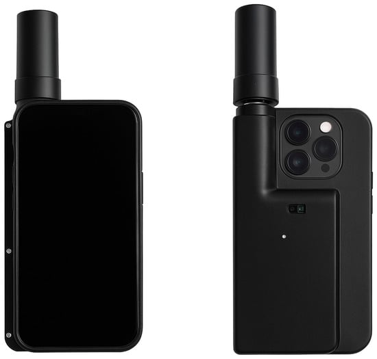
Figure 1. iPhone 15 Pro equipped with a viDoc GNSS receiver.

These phones are equipped with a time-of-flight (ToF) sensor that emits infrared rays in a predefined regular pattern [18]. In addition, these phones rotate between two patterns over time. This feature makes it possible to obtain more detailed information about image depth (more accurate determination of the distance of an object from the sensor). When a picture is taken, a laser measurement is also performed, which is then stored as additional information for the pictures [19]. In the case of Pix4Dcatch software, which was used during the study and is fully compatible with the viDoc device, three types of files are generated for each picture. These are the image itself in *.jpg format (with a resolution of 3024 × 4032 px), a depth image from the laser sensor in *.tiff format (resolution 256 × 192 px), and information about the reliability of the depth information obtained (values 0, 1, 2) in *.tiff format [20]. The depth reliability map assigns a value between 0 and 2 to each pixel. Higher values indicate more reliable laser depth measurements according to Pix4D’s internal quality model.

The viDoc device can be described as a compact GNSS receiver that is attached to the rear of the sensor during measurement and maintains a connection with it via Bluetooth protocol. For the purposes of this measurement, DGNSS RTK corrections were received from the CZEPOS network using VRS3-iMAX-MSM (a virtual reference station generated according to the individualized MAX concept with corrections from the GPS, GLONASS, Galileo, and BeiDou satellite systems) [21]. To clarify, CZEPOS is a network of stations uniformly distributed throughout the Czech Republic. The stations continuously record data from global navigation satellite systems.

Several proprietary software tools were used to process the data obtained from the measurements, including Pix4Dcatch, Pix4Dmatic, and Pix4Dsurvey [22,23,24]. These tools were selected primarily due to the common supplier of the entire solution, built-in support for outputs from the viDoc GNSS receiver, and a clearly defined and integrated workflow for data collection, processing, and analysis.

Measuring instruments commonly used in geodetic and geomatic practice were used for analysis and to obtain comparative data. These included a Leica GS18 T LTE GNSS receiver with a CS20 field controller [25] and a Leica RTC360 terrestrial laser scanner [26].

The main advantages of the Leica GNSS receiver include a wide measurement frequency range (up to 100 Hz) and the use of data from four satellite systems (GPS, GLONASS, Galileo, and BeiDou) [25]. As for the laser scanner, its key advantage lies in the use of two wavelengths for measurement [26]. The result is reduced noise on problematic surfaces, which is quite common in traffic accident investigations. These include, in particular, shiny car body surfaces, headlights, and glass.

Data from the comparison devices were again processed using proprietary software. This mainly involved Leica Infinity software (version 3.0.1) [27] and Leica Cyclone Register 360+ (2023.1.0. Build r.26401) [28]. The resulting point clouds were then compared using the open-source software CloudCompare (2.12.4. Kyiv) [29].

2. Method

Figure 2 provides an overview of the complete workflow used in this study, from the preparation of the test environment to the final accuracy evaluation. The procedure begins with the setup of the hybrid mobile device consisting of an iPhone and a viDoc GNSS receiver. The first test evaluates the accuracy of line measurements, while the second test verifies the accuracy when surveying larger traffic areas. In order to make a mutual comparison with highly accurate reference data, control measurements were performed using geodetic equipment and a terrestrial laser scanner. The acquired datasets were then exported, processed using specialized software, and subsequently compared with the reference measurements.

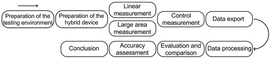
Figure 2. Overview of the methodological workflow used in this study.

2.1. Line Measurement

The scenario simulated a characteristic problem where accident traces are predominantly located in one direction, e.g., in the direction of vehicle travel. This is a typical measurement method that is not particularly suitable for hybrid data collection. Nevertheless, the approach enables an effective evaluation of the device’s suitability and allows the quantification of potential error propagation.

The measurements were taken at two locations with different surface structures (Figure 3). The first location was on an asphalt road with a subtle texture (series A). The second location had a mixed surface with a distinct texture consisting of granite cubes and horizontal road markings (series B). A strip with marked points was placed along the measurement axis. A total of 6 points were marked at 5 m intervals over a length of 25 m.

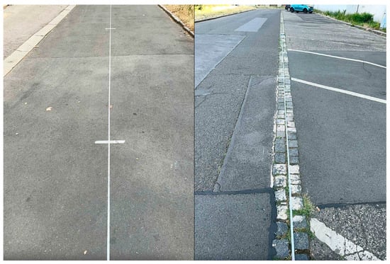
Figure 3. Line measurement and surface structure of Location A (left side of the picture) and Location B (right side of the picture).

The measurement also aimed to verify the influence of longitudinal slope. Traffic accidents occur on all types of roads, and lower-category roads in particular can have significant longitudinal slopes. Location A was situated in a place with a relatively high longitudinal slope of approximately 6.5%. Location B, on the other hand, was almost flat (elevation difference of up to 50 mm over a distance of 25 m).

The orientation of the images was performed similarly to typical imaging for terrestrial photogrammetry. Imaging was performed gradually with the sensor positioned at eye level and the images rotated so that the horizon was at the top edge of the image. The speed of movement was set to a slow walking pace. The coordinate system of the project was ETRS89 (EPSG 4258) [30].

A total of 7 measurements were performed in Series A and 5 measurements in Series B. The measurements differed in the method of image acquisition and the use or non-use of a GNSS receiver. The measurements are shown in Table 1.

Table 1. Line measurement—overview of settings for individual series of measurements.

ID	Trigger Method	Surface	RTK	Number of Images	Measured Distance
1A	Device Pose—1 m	Asphalt	YES	28	25 m
2A_RTK	Device Pose—1 m	Asphalt	NO	27	25 m
3A	Device Pose—10 cm	Asphalt	NO	274	25 m
4A_RTK	Device Pose—10 cm	Asphalt	YES	264	25 m
5A_RTK	Image Overlap—90%	Asphalt	YES	143	25 m
6A	Image Overlap—90%	Asphalt	NO	121	25 m
7A_RTK	Image Overlap—90%, faster walk	Asphalt	YES	103	25 m
1B	Device pose—10 cm	Granite	NO	337	25 m
2B_RTK	Device pose—10 cm	Granite	YES	291	25 m
3B_RTK	Image Overlap—90%, faster walk	Granite	YES	162	25 m
4B_RTK	Image Overlap—90%	Granite	YES	227	25 m
5B	Image Overlap—90%	Granite	NO	290	25 m

The software used provides access to information about the sensor’s position and orientation (Device Pose). If there is a significant change in the orientation of the sensor, additional photos are taken. The second method is to define the desired overlap of individual images (Image Overlap) [3]. This setting is essential for subsequent spatial reconstruction through digital image correlation, which is directly influenced by the degree of overlap between individual images.

After acquiring and processing the data, an evaluation of the achieved quality and observed deviations was performed. Two methodologically different approaches were chosen. The first was to work directly with the point cloud, where manual identification of the signaled points on individual images was performed. The output is thus information about the position of points in the coordinate system.

The second method was graphic processing, using the resulting orthophoto of the given line. The distance between points was therefore measured on this image. Orthophotos were chosen because they represent a typical measurement output that is further used in police or forensic investigations.

2.2. Evaluation of Line Measurements from the Point Cloud

The evaluation was divided into an analysis of deviations in the full 3D space (XYZ) and an analysis limited to the horizontal plane (XY). The reason for this is that traditional outputs and measurements by the police are usually only dealt with in the plane of the road. Height information is only provided for serious traffic accidents using modern measurement methods (total stations, GNSS receivers, or laser scanning). Evaluation without taking slope into account is closer to traditional outputs. In contrast, longitudinal slope provides information about the actual accuracy achieved.

The results of the horizontal measurements can be seen in Table 2, Table 3 and Table 4, and Figure 4, Figure 5 and Figure 6. Both the deviation in distance between individual points and the cumulative deviation were monitored. This makes it possible to evaluate both the accuracy achieved and the propagation of errors with increasing measurement length.

Table 2. Line measurement—evaluation of distance deviations between points in the XY plane.

XY Plane—5 m Segments				Sections [m]
ID	Method	RTK	Surface	Error from Known Distance of 5 m [mm]					Mean	Std. Dev.
1A	Device Pose—1 m	NO	asphalt	−62	−46	−81	−81	−70	−68	15
2A_RTK	Device Pose—1 m	YES	asphalt	−5	−58	−14	−93	−72	−48	38
3A	Device Pose—10 cm	NO	asphalt	−71	−65	−59	−43	15	−45	35
4A_RTK	Device Pose—10 cm	YES	asphalt	−24	−27	−56	−72	−80	−52	26
5A_RTK	Overlap	YES	asphalt	−25	−36	−52	−50	−8	−34	18
6A	Overlap	NO	asphalt	−73	−82	−45	−33	−21	−51	26
7A_RTK	Overlap	YES	asphalt	−42	−18	−38	−45	−40	−37	11
1B	Device pose	NO	granite	−28	3	31	49	70	25	39
2B_RTK	Device pose	YES	granite	−15	−13	−26	−35	−39	−26	12
3B_RTK	Overlap	YES	granite	−17	−18	−11	−18	−19	−17	3
4B_RTK	Overlap	YES	granite	−13	−21	−13	−16	−17	−16	3
5B	Overlap	NO	granite	9	24	28	27	48	27	14

Table 3. Line measurement—evaluation of cumulative distance deviations between points (XY plane).

XY Plane				Sections [m]
				Cumulative Error [mm]
ID	Method	RTK	Surface	0	5	10	15	20	25
1A	Device Pose—1 m	NO	asphalt	0	−62	−108	−189	−270	−340
2A_RTK	Device Pose—1 m	YES	asphalt	0	−5	−63	−77	−170	−242
3A	Device Pose—10 cm	NO	asphalt	0	−71	−136	−195	−238	−223
4A_RTK	Device Pose—10 cm	YES	asphalt	0	−24	−51	−107	−179	−259
5A_RTK	Overlap	YES	asphalt	0	−25	−61	−113	−163	−171
6A	Overlap	NO	asphalt	0	−73	−155	−201	−234	−255
7A_RTK	Overlap	YES	asphalt	0	−42	−60	−98	−144	−184
1B	Device pose	NO	granite	0	−28	−25	6	55	125
2B_RTK	Device pose	YES	granite	0	−15	−28	−54	−89	−128
3B_RTK	Overlap	YES	granite	0	−17	−35	−46	−64	−84
4B_RTK	Overlap	YES	granite	0	−13	−35	−48	−63	−80
5B	Overlap	NO	granite	0	9	33	61	87	135

Table 4. Line measurement—evaluation of relative distance deviations between points in the XY plane.

XY Plane—Relative				Sections [m]
				Cumulative Error [%]
ID	Method	RTK	Surface	0	5	10	15	20	25	Mean	STD	RMSE	MAE
1A	Device Pose—1 m	NO	asphalt	0.0	−1.2	−1.1	−1.3	−1.4	−1.4	−1.28	0.13	1.29	1.28
2A_RTK	Device Pose—1 m	YES	asphalt	0.0	−0.1	−0.6	−0.5	−0.9	−1.0	−0.62	0.36	0.70	0.62
3A	Device Pose—10 cm	NO	asphalt	0.0	−1.4	−1.4	−1.3	−1.2	−0.9	−1.24	0.21	1.25	1.24
4A_RTK	Device Pose—10 cm	YES	asphalt	0.0	−0.5	−0.5	−0.7	−0.9	−1.0	−0.72	0.23	0.75	0.72
5A_RTK	Overlap	YES	asphalt	0.0	−0.5	−0.6	−0.8	−0.8	−0.7	−0.68	0.13	0.69	0.68
6A	Overlap	NO	asphalt	0.0	−1.5	−1.6	−1.4	−1.2	−1.0	−1.34	0.24	1.36	1.34
7A_RTK	Overlap	YES	asphalt	0.0	−0.9	−0.6	−0.7	−0.7	−0.7	−0.72	0.11	0.73	0.72
1B	Device pose	NO	granite	0.0	−0.6	−0.3	0.0	0.3	0.5	−0.02	0.44	0.40	0.02
2B_RTK	Device pose	YES	granite	0.0	−0.3	−0.3	−0.4	−0.4	−0.5	−0.38	0.08	0.39	0.38
3B_RTK	Overlap	YES	granite	0.0	−0.3	−0.3	−0.3	−0.3	−0.3	−0.30	0.00	0.30	0.30
4B_RTK	Overlap	YES	granite	0.0	−0.3	−0.4	−0.3	−0.3	−0.3	−0.34	0.05	0.34	0.34
5B	Overlap	NO	granite	0.0	0.2	0.3	0.4	0.4	0.5	0.36	0.11	0.37	0.36
Device pose—no RTK										−0.85	0.26	0.98	0.95
Device pose—RTK										−0.57	0.22	0.61	0.57
Overlap—no RTK										−0.49	0.18	0.87	0.85
Overlap—RTK										−0.51	0.07	0.52	0.51

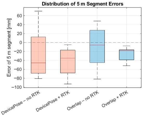
Figure 4. Distribution of errors for different acquisition modes and RTK configurations (Orange color—device pose setting method, blue color—overlap setting method. Red line—median).

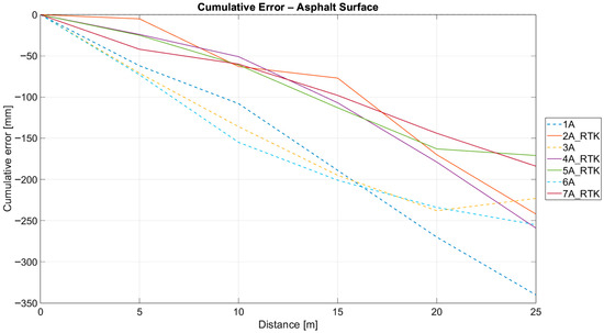
Figure 5. Line measurement—evaluation of distance deviations between points in the XY plane—Asphalt.

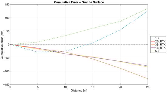
Figure 6. Line measurement—evaluation of distance deviations between points in the XY plane—Granite.

Table 2 and Figure 4 illustrate the error distribution for each 5 m segment. The results show clear differences between the DevicePose and Overlap modes, as well as between measurements with and without RTK. The largest variability and the highest negative deviations were observed in the DevicePose mode without RTK, where the median error reached –46 mm and individual segments exceeded –80 mm. The use of RTK in the same mode reduced both the variance and the magnitude of errors, although the variability remained relatively high. The Overlap mode showed more stable results. In combination with RTK, the variance narrowed significantly and the mean error approached –18 mm. It also exhibited no extreme outliers. These findings demonstrate that the availability of RTK corrections have a direct and significant impact on the accuracy of linear measurements.

Table 3 shows the cumulative deviations along the 25 m line for all tested configurations. The largest deviation occured in the DevicePose mode without RTK, where the cumulative error reached up to –340 mm. On the asphalt surface, the cumulative deviations showed an almost linear increase with distance, indicating systematic error propagation. The use of RTK reduced this drift, but cumulative deviations remained significant. In contrast, the Overlap mode produced more stable results, especially with RTK, where cumulative errors stayed below –185 mm on asphalt and below –85 mm on granite. The granite surface generally showed lower error accumulation due to better texture. Overall, the results show that both surface type and capture settings strongly affect long-distance accuracy. The best capture configuration is the Overlap + RTK, which shows the most consistent performance.

Table 4 summarizes the relative cumulative errors along the 25 m line for all configurations and shows clear differences between scanning modes, surface types, and RTK availability. On the asphalt surface, measurements without RTK produced the largest deviations (between –0.9% and –1.5%), which corresponds to cumulative errors of up to −340 mm. Using RTK reduced these errors to approximately −0.6% to −0.75%, demonstrating a substantial improvement in accuracy. On the granite surface, where the richer texture offers more reliable image matching, the deviations were considerably smaller and more stable. The Overlap with RTK configuration provided the most consistent performance, with nearly constant errors around −0.3% and minimal variability.

A two-sample t-test comparing RTK and non-RTK measurements showed that the difference between the two groups is highly statistically significant (p < 1 × 10⁻⁶). This confirms that RTK corrections have a strong and systematic positive effect on distance accuracy in hybrid mobile scanning.

The results of the spatial evaluation can be seen in Table 5. These tables show the difference in the resulting deviation with consideration of terrain slope.

Table 5. Line measurement—evaluation of cumulative distance deviations between points in 3D space.

5 m Segments				Cummulative Error Difference [mm]
ID	METHOD	RTK	SURFACE	0 m	5 m	10 m	15 m	20 m	25 m
1A	Device Pose—1 m	NO	asphalt	0	−14	−29	−47	−55	−57
2A_RTK	Device Pose—1 m	YES	asphalt	0	−7	−17	−33	−46	−60
3A	Device Pose—10 cm	NO	asphalt	0	−6	−16	−34	−52	−64
4A_RTK	Device Pose—10 cm	YES	asphalt	0	−5	−12	−27	−40	−50
5A_RTK	Overlap	YES	asphalt	0	−4	−12	−27	−42	−54
6A	Overlap	NO	asphalt	0	−4	−13	−28	−43	−55
7A_RTK	Overlap	YES	asphalt	0	−5	−13	−28	−42	−54
1B	Device pose	NO	granite	0	0	0	0	0	0
2B_RTK	Device pose	YES	granite	0	0	0	0	−1	−1
3B_RTK	Overlap	YES	granite	0	0	0	0	0	0
4B_RTK	Overlap	YES	granite	0	0	0	0	0	0
5B	Overlap	NO	granite	0	0	0	0	0	0

The findings clearly indicate a reduction in overall deviations at Location A (road with a significant slope), whereas at Location B, the difference is negligible. When summed cumulatively, the error in height at Location A is up to 64 mm.

2.3. Evaluation of Line Measurements from the Orthophoto

The second method for evaluating measurement deviations was to use generated orthophotos. This approach was chosen because it is closest to traditional activities associated with the preparation of forensic expert reports related to traffic accidents.

The orthophotos were generated based on elevation data from digital surface models. The resolution of the orthophotos (Ground Sampling Distance—GSD) was set to 1 cm/px, which ensures that distances measured on the orthophotos can achieve centimeter-level precision. This is the resolution traditionally used in aerial photogrammetry performed by forensic experts or the police. Its advantages include easy work with scale, sufficient detail, and limited data requirements. Figure 7 shows examples of generated orthophotos of both locations.

Figure 7. Final orthophotos of Location A and B (Location A—upper part of the image. Location B—lower part of the image).

The following Table 6 and Table 7 show the overall error rates for each measurement method.

Table 6. Line measurement—evaluation of distance deviations from the orthophoto.

Ortophoto—5 m Segments				Sections [m]
ID	Method	RTK	Surface	Error from Known Distance of 5 m [mm]					Mean	Std. Dev.
1A	Device Pose—1 m	NO	asphalt	-	−108	−59	−53	−52	−68	27
2A_RTK	Device Pose—1 m	YES	asphalt	-	−51	−36	−119	37	−42	64
3A	Device Pose—10 cm	NO	asphalt	−74	−72	−52	−46	−30	−55	18
4A_RTK	Device Pose—10 cm	YES	asphalt	−18	−38	−47	−79	−74	−51	25
5A_RTK	Overlap	YES	asphalt	−43	−39	−50	−48	−21	−40	12
6A	Overlap	NO	asphalt	−74	−81	−46	−36	−23	−52	25
7A_RTK	Overlap	YES	asphalt	−28	−25	−24	−51	−49	−35	13
1B	Device pose	NO	granite	−26	7	22	49	69	24	37
2B_RTK	Device pose	YES	granite	−9	−18	−23	−39	−44	−27	15
3B_RTK	Overlap	YES	granite	−16	-	−30	−20	−19	−21	6
4B_RTK	Overlap	YES	granite	−36	4	−16	−18	−16	−16	14
5B	Overlap	NO	granite	14	21	23	31	50	28	14

Table 7. Line measurement—evaluation of cumulative distance deviations from the orthophoto.

Ortophoto				Sections [m]
				Cummulative Error [mm]
ID	Method	RTK	Surface	0	5	10	15	20	25
1A	Device Pose—1 m	NO	asphalt	-	0	−108	−167	−220	−272
2A_RTK	Device Pose—1 m	YES	asphalt	-	0	−51	−87	−206	−169
3A	Device Pose—10 cm	NO	asphalt	0	−74	−146	−198	−244	−274
4A_RTK	Device Pose—10 cm	YES	asphalt	0	−18	−56	−103	−182	−256
5A_RTK	Overlap	YES	asphalt	0	−43	−82	−132	−180	−201
6A	Overlap	NO	asphalt	0	−74	−155	−201	−237	−260
7A_RTK	Overlap	YES	asphalt	0	−28	−53	−77	−128	−177
1B	Device pose	NO	granite	0	−26	−19	3	52	121
2B_RTK	Device pose	YES	granite	0	−9	−27	−50	−89	−133
3B_RTK	Overlap	YES	granite	0	−16	-	−46	−66	−85
4B_RTK	Overlap	YES	granite	0	−36	−32	−48	−66	−82
5B	Overlap	NO	granite	0	14	35	58	89	139

Similarly to Table 2, Table 6 and Figure 8 show the distribution of deviations measured for individual 5 m sections. The results clearly show the differences between DevicePose mode and Overlap mode. The DevicePose mode without RTK showed the greatest variability of errors. The median was −49 mm, and one section showed deviation of up to −108 mm. Enabling RTK in the same mode led to a reduction in the range and size of negative outliers, although the overall variability remained relatively high.

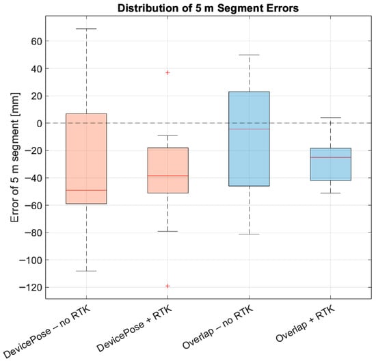
Figure 8. Distribution of errors for different acquisition modes and RTK configurations (orthophoto) (Orange color—device pose setting method, blue color—overlap setting method, Red line—median, Red cross—outliers).

Overlap mode, on the other hand, showed more stable results. Without RTK, the measurement dispersion was greater. However, the use of RTK significantly narrowed the distribution of deviations, making this configuration the most balanced and stable of all the cases studied. The occurrence of outliers was limited and the overall variability decreased significantly.

The findings clearly confirm that the availability of RTK corrections has a significant positive effect on the accuracy of length measurements and that Overlap mode in combination with RTK provides the most accurate and least variable results.

The following Table 7 shows the cumulative errors on the measured section and the subsequent plotting of the cumulative errors in Figure 9 and Figure 10.

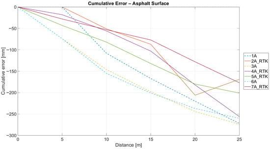
Figure 9. Line measurement—evaluation of distance deviations from the orthophoto of asphalt surface.

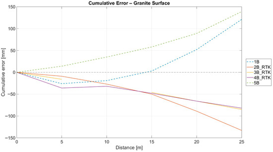
Figure 10. Line measurement—evaluation of distance deviations from the orthophoto of granite surface.

The cumulative errors measured on asphalt and granite surfaces show significant differences. On asphalt, all configurations without RTK tend to gradually increase to significantly negative values (Device Pose without RTK up to −274 mm). RTK corrections then demonstrably reduce the length error. The highest-quality orthophoto was again created from the Overlap configuration with RTK, which shows the smallest increasing error. The situation is different on granite surfaces. Methods without RTK often show positive drift (e.g., Overlap without RTK up to +139 mm), while methods with RTK show a predominantly negative trend with less variability. The most consistent results are provided by Overlap variants with RTK (errors between −16 and −85 mm) and show the smallest variance. The Overlap mode is the most reliable for linear measurements in both surface conditions, and the results show a very similar trend to the point cloud (Table 3).

2.4. Control Points

In the case of larger areas, even a small relative deviation quickly becomes problematic. Therefore, control points with known positions are usually used in photogrammetric imaging. CPs then ensure both solution control and information about the deviations achieved. The Pix4Dcatch software [22] allows for the measurement of control points when a viDoc GNSS receiver is connected. The accuracy of the control point measurements was tested and compared with the Leica GS18 GNSS [25].

Two groups of points were created within the Pix4Dcatch software [22]. The first was for points measured in the S-JTSK coordinate system with the Baltic vertical system after adjustment (Bpv)—EPSG 5514 + 8357. To clarify, S-JTSK is the official geodetic reference system in the Czech Republic. S-JTSK is defined in the Křovák projection plane (double conformal conical projection in general position) [30]. Bpv is a vertical system representing heights derived from the Baltic Sea after the 1957 adjustment. The starting elevation point is zero on the sea level scale in Kronstadt.

The second group of points was surveyed using The European Terrestrial Reference System 1989 (ERTS89) coordinate system—with code EPSG 4258 [30]. The software allowed for a choice of measurement intervals above the point of 5, 15, and 30 s. Ten measurements were taken for each time group. A Leica GS18 GNSS receiver was used for comparative measurements. The deviations in the determined position can be seen in the following Table 8.

Table 8. Control points—Positional deviations of measured points using viDoc GNSS receiver.

viDoc	ETRS			S-JTSK			S-JTSK (CUZK)
	Longitude [m]	Latitude [m]	Height [m]	Y [m]	X [m]	Z [m]	Y [m]	X [m]	Z [m]
5s_01	0.009	−0.095	−0.010	0.156	−0.123	0.292	0.059	−0.022	−0.010
5s_02	−0.004	−0.084	−0.020	0.148	−0.114	0.287	0.054	−0.001	−0.020
5s_03	0.020	−0.037	0.003	0.172	−0.101	0.287	0.019	−0.035	0.003
5s_04	0.030	−0.045	0.000	0.146	−0.104	0.292	0.022	−0.051	0.000
5s_05	0.017	−0.042	−0.006	0.147	−0.113	0.288	0.023	−0.029	−0.006
5s_06	0.013	−0.025	−0.001	0.141	−0.096	0.296	0.013	−0.022	−0.001
5s_07	0.021	−0.061	0.032	0.151	−0.094	0.302	0.035	−0.039	0.033
5s_08	0.028	−0.068	0.024	0.135	−0.088	0.299	0.037	−0.049	0.024
5s_09	0.019	−0.054	0.016	0.097	−0.067	0.303	0.030	−0.034	0.016
5s_10	−0.015	−0.049	−0.010	0.153	−0.093	0.311	0.034	0.020	−0.010
15s_01	−0.002	−0.046	−0.020	0.132	−0.095	0.307	0.030	0.000	−0.020
15s_02	−0.005	−0.012	−0.018	0.155	−0.105	0.303	0.008	0.007	−0.018
15s_03	0.010	0.009	−0.027	0.158	−0.111	0.306	−0.008	−0.015	−0.027
15s_04	0.002	0.013	−0.027	0.155	−0.103	0.318	−0.009	−0.003	−0.026
15s_05	−0.003	0.019	−0.030	0.152	−0.100	0.311	−0.011	0.006	−0.030
15s_06	−0.021	0.069	−0.035	0.142	−0.093	0.317	−0.039	0.039	−0.035
15s_07	−0.015	0.044	−0.036	0.118	−0.067	0.333	−0.025	0.028	−0.036
15s_08	−0.016	0.023	−0.037	0.144	−0.076	0.335	−0.011	0.027	−0.037
15s_09	−0.013	0.062	−0.034	0.146	−0.075	0.334	−0.037	0.026	−0.034
15s_10	−0.014	0.065	−0.035	0.157	−0.068	0.352	−0.039	0.027	−0.035
30s_01	−0.009	0.053	−0.036	0.151	−0.071	0.352	−0.032	0.019	−0.036
30s_02	−0.010	0.070	−0.032	0.150	−0.067	0.385	−0.043	0.021	−0.032
30s_03	−0.006	0.056	−0.032	0.137	−0.051	0.367	−0.034	0.013	−0.032
30s_04	−0.007	0.049	−0.026	0.131	−0.033	0.374	−0.029	0.016	−0.026
30s_05	0.005	0.010	−0.035	0.139	−0.046	0.372	−0.008	−0.006	−0.034
30s_06	0.005	0.036	−0.029	0.119	−0.038	0.388	−0.024	−0.005	−0.028
30s_07	0.005	0.019	−0.028	0.121	−0.037	0.392	−0.014	−0.006	−0.028
30s_08	0.004	0.026	−0.027	0.147	−0.045	0.398	−0.018	−0.004	−0.026
30s_09	0.002	0.009	−0.029	0.106	−0.028	0.405	−0.007	−0.002	−0.028
30s_10	−0.010	0.046	−0.033	0.093	−0.021	0.425	−0.027	0.019	−0.033
5s agregated	0.018	0.056	0.012	0.145	0.099	0.296	0.033	0.030	0.012
15s agregated	0.010	0.036	0.030	0.146	0.089	0.321	0.022	0.018	0.030
30s agregated	0.006	0.037	0.031	0.129	0.044	0.386	0.024	0.011	0.030
Mean	0.001	0.002	−0.019	0.140	−0.077	0.334	−0.002	−0.002	−0.020
STD	0.014	0.050	0.019	0.019	0.029	0.041	0.030	0.025	0.019
RMSE	0.014	0.049	0.027	0.141	0.083	0.337	0.029	0.024	0.027
MAE	0.011	0.043	0.024	0.140	0.077	0.334	0.026	0.020	0.0241

The results show errors in the transformation key for the S-JTSK and Bpv coordinate systems used in the Czech Republic. The reason is that Pix4D software is not on the list of transformation programs approved by the Czech Office for Surveying, Mapping and Cadastre (ČÚZK). The transformation key used thus leads to deviations when using the S-JTSK coordinate system, especially in the specified height compared to reality. Although the Czech CR-2005 geoid was implemented in the software with version 1.59, the height deviations are not insignificant. For this reason, a test was conducted to transform coordinates measured in the ETRS89 coordinate system via the ČÚZK online portal [31] to S-JTSK (Table 8, third column). By using the correct transformation key, the problem was essentially eliminated.

In terms of measurement time when using the viDoc device, it appears that although longer measurement times lead to lower errors, the difference between 15 s and 30 s is already at the limit of the device’s achievable positional accuracy. The difference in measurement accuracy between the Leica GS 18 and viDoc devices is to be expected and can be explained by the dimensions of the antenna and the primary focus of the individual devices. Based on the measurements taken, the accuracy achieved by the hybrid device appears to be sufficient for use in documenting traffic accident sites.

2.5. Documentation of the Larger Scene

Based on previous measurements, a series of larger-scale comparative measurements was also carried out. The aim was to verify the possibility of using control points (CP) to increase the accuracy of measurements, analyze the characteristics of the outputs, and verify the behavior of the technology under extreme conditions. At the same time, the time required for processing and the quality of the output data for possible further use in the analysis of traffic accidents was also monitored.

A road with a significant slope and directional profile was selected for testing. At the same time, there were a number of objects of interest in the area that are often documented in traffic accidents (traffic signs, public lighting). Since the influence of DGNSS was being tested, part of the measured area was located near buildings and part in an open area with an unrestricted view of the sky.

Measurements using a terrestrial laser scanner Leica RTC360 and a GNSS receiver Leica GS18 were used as reference measurements. Control points were placed on plywood boards within the area to maintain shape stability and limit their movement due to wind. Each point was surveyed using a Leica GNSS device and viDoc. The surveyed positions of the control points using GNSS measurements were then used in a comparative analysis.

The tested scenarios of a larger traffic accident site were divided into two groups. The measurement settings were made based on previous findings (Image Overlap 90%). Imaging was performed in more directions, back and forth, with a smooth rotation at both extreme positions for maximum continuity of images.

The first group consisted of measurements under ideal conditions (Test01). The influence of control points on the achieved deviations and the form of the outputs was tested. In the second case (Test02), measurements were performed with lower positioning accuracy of the images. During imaging, the positional accuracy was indicated as approximately 1 m. The reason for this is that in many cases, traffic accidents occur in areas where signal reception is not ideal (e.g., wooded areas, near high-rise buildings, etc.). In this case, the location was imaged in greater detail—three imaging lanes. Both examples can be seen in Figure 11.

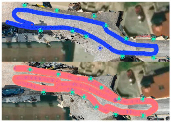
Figure 11. Larger scene—Image configuration (Test 01 and Test 02) with control points locations marked (Blue trajectory—use of 90% image overlap. Red trajectory—use of 1 m positional accuracy. Green points—control points).

2.6. Test 01

The processing was performed using identical input data. This involved comparative measurements using a Leica RTC 360 terrestrial laser scanner and a hybrid scanning device iPhone 15 Pro. The difference was in the use of different sources of positional information for control points. In the first case, positions determined by a Leica GNSS receiver (Test01gnss) were used (Figure 12 and Figure 13), in the second case by a viDoc GNSS receiver (Test01viDoc, see Figure 14 and Figure 15), and in the third case, no control points were used to align the scans (Figure 16 and Figure 17).

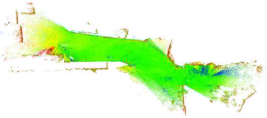
Figure 12. Test 01—Graphical representation of identified XYZ deviations of control points measured using Leica TS 18 GNSS.

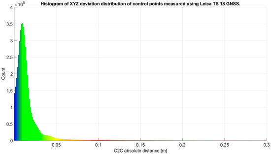
Figure 13. Test 01—Histogram of XYZ deviation distribution of control points measured using Leica TS 18 GNSS.

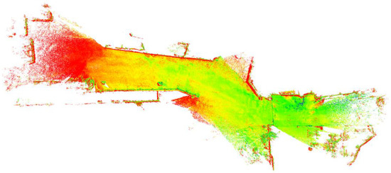
Figure 14. Test 01—Graphical representation of identified XYZ deviations of control points measured using viDoc.

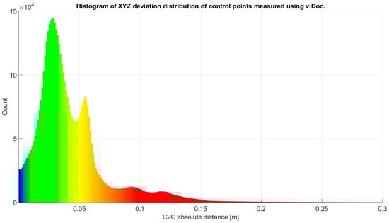
Figure 15. Test 01—Histogram of XYZ deviation distribution of control points measured using viDoc.

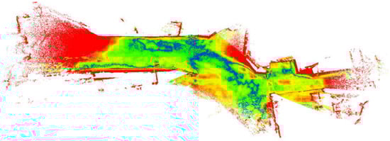
Figure 16. Test 01—Graphical representation of identified XYZ deviations, no control points.

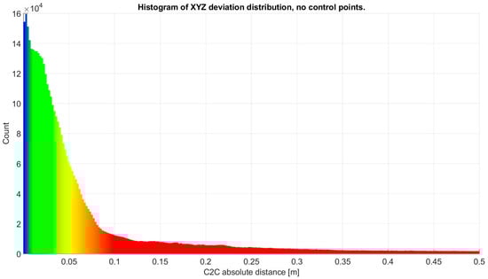
Figure 17. Test 01—Histogram of XYZ deviation distribution, no control points.

2.7. Test 02

The second evaluation was performed with regard to the influence of deteriorated measurement conditions (low positional accuracy of image determination). The resulting indicated deviation of image position determination was in the range of 80 to 110 cm. For comparison, it can be said that the indicated deviation in the first test was from 1 to 3 cm.

The processing was performed similarly to the first case, i.e., using the same data. The aim was to monitor the influence of the quality and presence of targets on the results achieved, as in the first case. Figure 18 and Figure 19 show the effect of control points measured using GNSS Leica TS 18, Figure 20 and Figure 21 show the effect of control points using viDoc, Figure 22 and Figure 23 do not use control points.

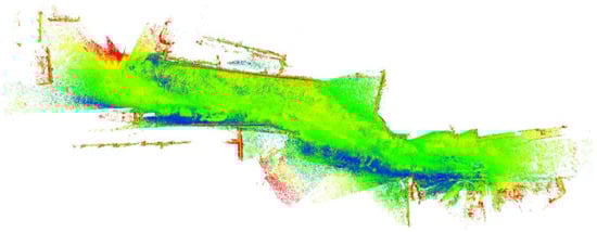
Figure 18. Test 02—Graphical representation of identified XYZ deviations of control points measured using GNSS Leica TS 18.

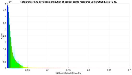
Figure 19. Test 02—Histogram of XYZ deviation distribution of control points measured using GNSS Leica TS 18.

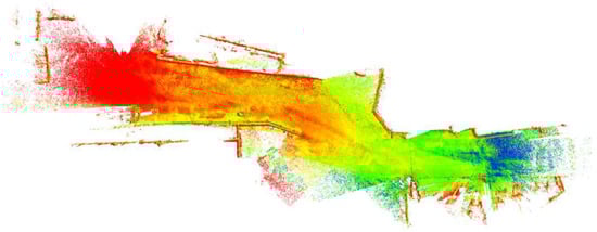
Figure 20. Test 02—Graphical representation of identified XYZ deviations of control points measured using viDoc.

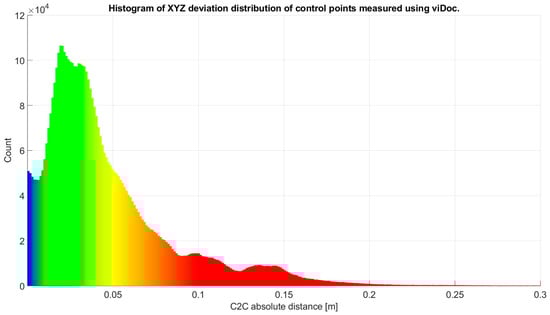
Figure 21. Test 02—Histogram of XYZ deviation distribution of control points measured using viDoc.

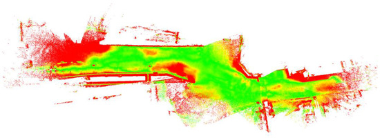
Figure 22. Test 02—Graphical representation of identified XYZ deviations, no control points.

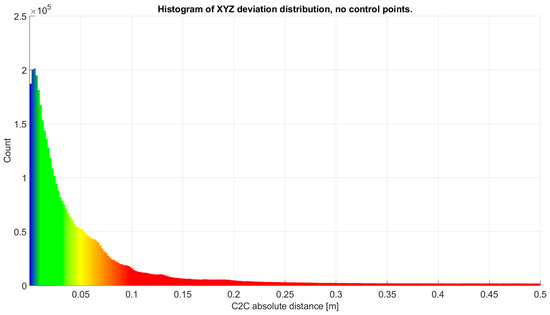
Figure 23. Test 02—Histogram of XYZ deviation distribution, no control points.

3. Results

Table 9 summarizes the results achieved and the deviations identified from the figures presented above. For each point cloud, the percentage of points with a deviation of up to 1 cm and up to 10 cm was calculated. In cases where control points were not used (Test01noCP, Test02noCP), the entire model was calculated in the ETRS89 coordinate system, which uses geographic (ellipsoidal) coordinates (latitude, longitude, height). Because such coordinates are not directly suitable for planar metric comparison,, the resulting point cloud is exported in the rectangular ETRS89 UTM 33N coordinate system, which is a projected metric system, and therefore it is not possible to make a direct comparison without alignment.

Table 9. Statistical evaluation of cloud-to-cloud deviations for Test 01 and Test 02.

	RMS [mm]	Percentage of Points Within Distance of		Z Deviation [mm]
		10 mm	100 mm	Mean	Sigma	RMS
Test01GNSS	39	46.06%	98.39%	11	20	23
Test01viDoc	62	6.75%	93.38%	33	28	44
Test01noGCP	ETRS89/UTM zone 33N—EPSG:25833
Test02GNSS	41	66.91%	98.66%	6	24	25
Test02viDoc	68	8.96%	89.25%	41	35	54
Test02noGCP	ETRS89/UTM zone 33N—EPSG:25833

The best results were achieved using the Leica TS 18 GNSS device. This solution has the lowest spatial RMS error. For Test01, the RMS is 39 mm, and for Test02, the RMS is 41 mm. At the same time, a relatively high percentage of points with a deviation of up to 10 mm is detected (46.06%—Test01, 66.91%—Test 02). These results show very good stability of the absolute spatial position of the model and overall high quality of its georeferencing. The elevation statistics further confirm that the Z component is very well determined when using GNSS control points (RMS—23–25 mm).

On the other hand, solutions using control points measured by the viDoc device show higher RMS values in space and, in particular, a significantly lower percentage of points with a deviation of up to 10 mm (6.75% and 8.96%). Although the absolute accuracy of these models is lower, the results show that the overall geometric consistency of the reconstruction is maintained. This is also supported by the high proportion of points within a tolerance of 100 mm. The resulting error is therefore mainly reflected in the absolute position, not in the shape of the reconstructed scene itself. Nevertheless, from the point of view of practical forensic documentation, hybrid data collection can be considered as a useful compromise in situations where it is not possible to use geodetic GNSS equipment.

The variants without control points cannot be fully included in the table because they are not directly comparable with the reference cloud. The absence of control points causes significant uncertainty in the scale, orientation, and absolute position of the model, which excludes the use of direct cloud-to-cloud analysis. At the same time, it is not possible to ensure a consistent and reproducible comparison of the outputs with other data. In order to ensure reproducibility, it would be possible to use the iterative closest point method, which minimizes the differences between point clouds by repeatedly searching for the closest points. The least squares method is used to estimate the optimal rotation and translation, which gradually minimizes the distances. The results of this comparison can be seen in Table 10.

Table 10. Statistical evaluation after fine alignment for Test 01 and Test.

	RMS [mm]	Percentage of Points Within Distance of		Z deviation [mm]
		10 mm	100 mm	Mean	Sigma	RMS
Test01GNSS	37	75.16%	98.43%	1	23	23
Test01viDoc	45	75.16%	98.43%	1	27	27
Test01noGCP	365	16.50%	81.21%	19	140	141
Test02GNSS	40	70.27%	98.76%	2	24	24
Test02viDoc	48	52.46%	94.47%	3	26	27
Test02noGCP	324	25.22%	83.12%	32	158	162

The results in Table 10 show the geometric deviation after fine alignment. Compared to the previous evaluation based on control points, the results are not affected by inaccurate georeferencing, but only by how well the individual methods were able to reconstruct the overall shape of the scene. This is why the RMS values are significantly reduced for all tests after fine alignment. The shift, rotation, and scale errors caused by imperfect georeferencing are eliminated.

The results show that the differences between GNSS and viDoc are significantly reduced. Both methods achieve very similar RMS values (37–48 mm). The geometric quality of the reconstructed cloud is significantly better with the viDoc solution than its absolute position would indicate. viDoc points therefore provide poorer georeferencing of control points, but the shape of the reconstructed scene itself is only slightly less accurate than with GNSS.

Tests without control points show the worst results even after fine alignment. The total RMS is 356 mm and 324 mm, and points with errors of up to 10 mm are only 16.50% and 25.22%. The point cloud still has a high degree of local deformations caused by the absence of control points during reconstruction. The significant metric uncertainty of these solutions is also clearly reflected in the RMS at height Z. The stability of models created in this way is low.

Overall, it can be said that the quality of the control points used significantly determines the final accuracy of the area reconstruction. GNSS points provide the best absolute and relative accuracy, while viDoc points allow for a geometrically stable, although less accurately referenced model. It has been confirmed that without control points, there is a significant deterioration in absolute position. If possible, it is not advisable to perform measurements without control points.

4. Discussion

Based on the conducted analyses, the usability of hybrid data collection with a GNSS receiver is possible, but mainly for accident sites with limited scope and complexity. With increasing size of the measured area, it is necessary to consider the gradually increasing measurement inaccuracy. When assessing a homogeneous surface, such as asphalt, it is possible to observe an almost linear increase in length error caused by image correlation limits.

When documenting traffic accident sites, it is useful to use control points, which increase the accuracy achieved. The importance of control points was also demonstrated in test measurements of large areas (Test 01 and Test 02). In situations where measurements were taken with control points, the models achieved significantly higher accuracy (up to 66.91% of points within 10 mm and 98.66% within 100 mm). This error may seem relatively high, but it is important to note that the current analysis was presented under very specific conditions of a homogeneous road surface. At the site of a real traffic accident, there will be a greater number of elements (vehicles, fragments) on the road that will help align the point cloud. Even if future tests show that the measurement error is still approximately 10 cm, this value can still be considered sufficiently accurate for the purpose of assessment.

If control points were missing during measurement, internal local deformations of the point cloud occurred, and the error rate increased significantly. In such cases, only 16.5% and 25.22% of points were measured within an error of 10 mm and 81.21% and 83.12% within 100 mm using the fine alignment method.

The study did not directly test how many control points are needed in the assessed location. This factor depends mainly on the size of the location and its complexity. The general recommendation, which was also applied in this study, is that the assessed location should be uniformly covered with control points to prevent local deformations. Another factor affecting the final number of points is the positional accuracy of GNSS measurements. If the measurements are taken in poor conditions with insufficient signal coverage, the number of usable points and the final accuracy of the point cloud for the given location may be affected. More detailed testing of the number of control points will be the subject of future analysis.

Currently, this technology is also being tested directly at the sites of specific traffic accidents. Due to the simplicity of measurement and affordability of this technology, its practical use is expected to become increasingly relevant. A major benefit is the large amount of information that can be obtained from the site of a traffic accident.

5. Conclusions

In conclusion, it can be said that the recommended setting for such devices is imaging based on image overlap (e.g., 90%). It is also recommended to take images at maximum resolution and use a GNSS receiver with a fixed position and scan the location in multiple directions.

The results of the analyses confirmed that hybrid data collection is most suitable for accident sites with a limited scope. The spread of errors increases proportionally with the size of the surveyed area. However, the study also showed that the use of control points significantly increases the geometric stability of the reconstruction. Even in less ideal scenarios, such as homogeneous asphalt surfaces, the measurement deviations achieved using hybrid scanning remained at a level acceptable for practical accident documentation.

Hybrid scanning can also be considered a suitable alternative to other measurement methods, such as comprehensive scanning using a terrestrial 3D scanner or scanning a given area using drones. These more sophisticated technologies require greater expertise in terms of their operation and evaluation. When investigating a traffic accident, a police officer is forced to perform several tasks in a very short time (assisting in rescuing people, securing the accident site, directing traffic, taking photographs). Hybrid scanning, therefore, allows a faster method of measurement than the above-mentioned methods.

References

- Jonassen, V.O.; Kjørsvik, N.S.; Blankenberg, L.E.; Gjevestad, J.G.O. Aerial Hybrid Adjustment of LiDAR Point Clouds, Frame Images, and Linear Pushbroom Images. Remote Sens. 2024, 16, 3179. [Google Scholar] [CrossRef]
- Haala, N.; Kölle, M.; Cramer, M.; Laupheimer, D.; Zimmermann, F. Hybrid georeferencing of images and LiDAR data for UAV-based point cloud collection at millimetre accuracy. ISPRS Open J. Photogramm. Remote Sens. 2022, 4, 100014. [Google Scholar] [CrossRef]
- Pix4D. Quick Start Guide: viDoc RTK Rover & PIX4Dcatch. 2025. Available online: https://data.pix4d.com/misc/KB/Getting+Started+PDFs/EN/Quick+Start+Guide+PIX4Dcatch+viDoc+RTK+rover+EN.pdf (accessed on 1 August 2025).
- Aksoy, E. Determining the usability of the ViDoc device, which integrates with smart phones, in documenting historical structures. Measurement 2025, 242, 116156. [Google Scholar] [CrossRef]
- Zhang, N.; Lan, X. Everyday-Carry Equipment Mapping: A Portable and Low-Cost Method for 3D Digital Documentation of Architectural Heritage by Integrated iPhone and Microdrone. Buildings 2024, 15, 89. [Google Scholar] [CrossRef]
- Rapuca, A.; Matoušková, E. Testing of Close-Range Photogrammetry and Laser Scanning for Easy Documentation of Historical Objects and Buildings Parts. Stavební Obz.-Civil Eng. J. 2023, 32, 504–518. [Google Scholar] [CrossRef]
- Demirel, Y.; Türk, T. Assessment of the Location Accuracy of Points Obtained with A Low-Cost Lidar Scanning System and GNSS Method. Mersin Photogramm. J. 2024, 6, 60–65. [Google Scholar] [CrossRef]
- Zollini, S.; Marconi, L. Evaluation of Positioning Accuracy Using Smartphone RGB and LiDAR Sensors with the viDoc RTK Rover. Sensors 2025, 25, 3867. [Google Scholar] [CrossRef] [PubMed]
- Nilnoree, S.; Mizutani, T. An innovative framework for incorporating iPhone LiDAR point cloud in digitized documentation of road operations. Results Eng. 2025, 25, 103953. [Google Scholar] [CrossRef]
- Miller, S.H.; Stogsdill, M.; McWhirter, S. Accuracy of Mobile Phone LiDAR on Crashed Vehicles; SAE Technical Paper Series; SAE International: Warrendale, PA, USA, 2025. [Google Scholar] [CrossRef]
- Sheshtar, F.M.; Alhatlani, W.M.; Moulden, M.; Kim, J.H. Comparative Analysis of LiDAR and Photogrammetry for 3D Crime Scene Reconstruction. Appl. Sci. 2025, 15, 1085. [Google Scholar] [CrossRef]
- Chase, C.E.; Liscio, E. Technical Note: Validation of Recon-3D, iPhone LiDAR for bullet trajectory documentation. Forensic Sci. Int. 2023, 350, 111787. [Google Scholar] [CrossRef] [PubMed]
- Tamimi, R.; Toth, C. Performance Assessment of a Mini Mobile Mapping System: Iphone 14 Pro Installed on a e-Scooter. In The International Archives of the Photogrammetry, Remote Sensing and Spatial Information Sciences; Copernicus Publications: Göttingen, Germany, 2023; Volume XLVIII-M-3-2023, pp. 307–315. [Google Scholar] [CrossRef]
- Kędziorski, P.; Skoratko, A.; Katzer, J.; Tysiąc, P.; Jagoda, M.; Zawidzki, M. Harnessing low-cost LiDAR scanners for deformation assessment of 3D-printed concrete-plastic columns with cross-sections based on fractals after critical compressive loading. Measurement 2025, 249, 117015. [Google Scholar] [CrossRef]
- Feudjio, S.L.T.; Fondzenyuy, S.K.; Ngwah, E.C.; Wounba, J.F.; Usami, D.S.; Persia, L. Traffic Conflict Approach in Road Safety: A Review of Data Collection Methods. Transp. Res. Procedia 2025, 90, 615–622. [Google Scholar] [CrossRef]
- Skaug, L.I.; Nojoumian, M. Llm-Assisted GIS Validation: A Computational Method for Improving Traffic Crash Location Data; Elsevier: Amsterdam, The Netherlands, 2025. [Google Scholar] [CrossRef]
- Liu, Y.; Wu, J.; Song, X. Pixel-wise anomaly detection on road by encoder–decoder semantic segmentation framework with driving vigilance. Comput.-Aided Civil Infrastruct. Eng. 2025, 40, 2190–2208. [Google Scholar] [CrossRef]
- Li, Y.; Liu, X.; Dong, W.; Zhou, H.; Bao, H.; Zhang, G.; Zhang, Y.; Cui, Z. DELTAR: Depth Estimation from a Light-weight ToF Sensor and RGB Image. arXiv 2022. [Google Scholar] [CrossRef]
- Kottner, S.; Thali, M.J.; Gascho, D. Using the iPhone’s LiDAR technology to capture 3D forensic data at crime and crash scenes. Forensic Imaging 2023, 32, 200535. [Google Scholar] [CrossRef]
- Pix4D. How to Process PIX4Dcatch Datasets in PIX4Dmatic. Pix4D Documentation. 2025. Available online: https://support.pix4d.com/hc/en-us/articles/4414523101073 (accessed on 31 July 2025).
- Czech Office for Surveying, Mapping and Cadastre (ČÚZK). Information About CZEPOS Services and Products. 2025. Available online: https://czepos.cuzk.cz/_servicesProducts.aspx (accessed on 1 August 2025).
- Pix4D. PIX4Dcatch Documentation. Pix4D Documentation. 2025. Available online: https://support.pix4d.com/hc/pix4dcatch (accessed on 31 July 2025).
- Pix4D. PIX4Dmatic Documentation. Pix4D Documentation. 2025. Available online: https://support.pix4d.com/hc/pix4dmatic (accessed on 31 July 2025).
- Pix4D. PIX4Dsurvey Documentation. Pix4D Documentation. 2025. Available online: https://support.pix4d.com/hc/pix4dsurvey (accessed on 31 July 2025).
- Leica Geosystems AG. Leica GS18 T Data Sheet. 2025. Available online: https://leica-geosystems.com/-/media/files/leicageosystems/products/datasheets/leica_gs18_t_ds_0325.ashx?sc_lang=sv-se&hash=CF1764F55DF5314A52FB9D409A24C7D6 (accessed on 1 August 2025).
- Leica Geosystems AG. Leica RTC360 3D Reality Capture Solution. 2025. Available online: https://leica-geosystems.com/products/laser-scanners/scanners/leica-rtc360 (accessed on 31 July 2025).
- Leica Geosystems AG. Leica Infinity Surveying Software. 2025. Available online: https://leica-geosystems.com/en-us/products/gnss-systems/software/leica-infinity (accessed on 31 July 2025).
- Leica Geosystems AG. Cyclone REGISTER 360 PLUS 2023.1.0 Release Notes. 2023. Available online: https://leica-geosystems.com/products/laser-scanners/software/leica-cyclone/leica-cyclone-register-360 (accessed on 31 July 2025).
- Montaut, G.G.; Daniel, G.M. CloudCompare—3D Point Cloud Processing Software. Available online: https://www.danielgm.net/cc/ (accessed on 31 July 2025).
- Czech Office for Surveying, Mapping and Cadastre (ČÚZK). Coordinate Reference Systems—Geoportal. Available online: https://geoportal.cuzk.cz/(S(qt0kuqjvvjvhrgv21p5eae1d))/Default.aspx?lng=EN&mode=TextMeta&text=souradsystemy&side=INSPIRE_SITsluzby&menu=43&head_tab=sekce-04-gp (accessed on 1 August 2025).
- Czech Office for Surveying, Mapping and Cadastre (ČÚZK). Coordinate Transformation Services (WCTS)—Geoportal. Available online: https://geoportal.cuzk.cz/(S(qt0kuqjvvjvhrgv21p5eae1d))/Default.aspx?lng=EN&head_tab=sekce-01-gp&mode=TextMeta&text=wcts&menu=19 (accessed on 1 August 2025).
Disclaimer/Publisher’s Note: The statements, opinions and data contained in all publications are solely those of the individual author(s) and contributor(s) and not of MDPI and/or the editor(s). MDPI and/or the editor(s) disclaim responsibility for any injury to people or property resulting from any ideas, methods, instructions or products referred to in the content. |
© 2025 by the authors. Licensee MDPI, Basel, Switzerland. This article is an open access article distributed under the terms and conditions of the Creative Commons Attribution (CC BY) license (https://creativecommons.org/licenses/by/4.0/).