Analysis of Shoreline Dynamics and Beach Profile Evolution over More than a Decade: Satellite Image Characterization and Machine Learning Modeling

Highlights

What are the main findings?

• The beach profiles in the Bocagrande sector of Cartagena de Indias exhibit temporal variability, influenced by both seasonal cycles and changes in the wave climate.
• The Rational Quadratic Gaussian Process Regression model, incorporating distance, season, year, month, and profile number, achieved high predictive accuracy (R² = 0.99) for estimating depths in beach profiles in the Bocagrande area of Cartagena de Indias, Colombia.

What is the implication of the main finding?

• The Bocagrande beach undergoes periodic accretion and erosion processes in the absence of construction activities.
• The integration of satellite imagery and beach profile measurements with machine learning enables the formulation of equilibrium profile equations.

Abstract

This study presents a detailed analysis of the morphological evolution of beaches in the Bocagrande sector of Cartagena de Indias, Colombia, over more than a decade, based on periodic monitoring of six beach profiles. The beaches in this area are in bays constrained by headlands and promontories located at both ends of each bay. Changes in shoreline position, dry beach widths, and the surf zone were evaluated using aerial photographs, orthophotos, satellite imagery, and field data, together with sediment size determined through granulometric analysis. The results indicate that the beaches exhibit characteristics of wave-dominated, exposed systems, with sediments classified as fine sand that tend to increase in grain size toward the northern sector of the bay. A cyclical variation in the shoreline was observed, with average retreats and advances ranging from 5 to 10 m, depending on the climatic season. Dry beach widths ranged from 10 to 90 m, decreasing toward the north. Differences in morphology between profiles and shoreline variation are attributed to the climatic season, profile location within the bay, and proximity to a coastal structure and its particular type. Beach profiles were fitted to conceptual equilibrium profile models using traditional equations, which yielded a coefficient of determination of 0.76; when machine learning algorithms were applied, this value improved to 0.99. This study provides an important baseline for future morphological assessments and coastal management efforts in the city and places with similar characteristics, particularly considering ongoing shoreline protection projects.

1. Introduction

In many coastal regions worldwide, particularly on low-lying sandy shores, tourism is a primary source of income for local populations, leading to residential and infrastructural development close to the shoreline [1]. Coastal zones are characterized by their dynamic nature and variability over short time periods, with waves, tides, and wind being the main drivers of these changes [2]. Coastal erosion and accretion are natural processes occurring on beaches [3]; however, they can become problematic when exacerbated by human activities or natural disasters. Beach erosion is a highly complex process that involves not only hydrodynamic conditions but also human influence. Coastal hard structures such as groins, jetties, seawalls, bulkheads, revetments, breakwaters, headlands, sills, and reefs are likely the dominant cause of human-induced coastal changes [4,5]. Even sand mining can cause shoreline erosion.

The equilibrium profile of a beach is the result of the balance between destructive and constructive forces in the environment, which depend on factors such as the type of seabed material, beach slope, and wave conditions [6]. If the balance between these forces is disrupted, the more potent force will dominate until the beach profile evolves and equilibrium is restored. When destructive forces prevail, the beach profile experiences erosion. Beach profiles vary over time, both seasonally and in response to long-term changes in the wave climate, leading to erosion or accretion. Embayed beaches are affected by cross-shore and long-shore sediment transport processes in the surf zone, which result in beach oscillation and rotation in the short-to-medium term [4,5,7]. Boundaries, both emerged and submerged, exert a primary control on wave shoaling processes, refraction–diffraction processes, and efficiency of longshore drift in a coast [4,5,8]. The sequence of storms also represents a potentially underestimated risk to beaches, as they can cause greater coastal erosion [4,5,9]. Therefore, it is utmost important to have field data of beach profiles at several points over time to assess the behavior of a beach [10,11].

Technological improvements have enabled the expansion and precision of coastal studies, and new statistical techniques for identifying trends, quasi-periodic behavior, and other measures of predictability continue to be developed. The vast amount of data collected from various studies and the development of new statistical techniques have enabled the creation of new tools that offer alternatives to commonly used modeling methods. The integration of machine learning (ML) techniques into coastal engineering represents a significant shift in how coastal processes are modeled and understood [12].

Cartagena de Indias is located along the central part of the Caribbean coast of Colombia, between the coordinates 75°30.07′ W and 10°29.87′ N, and 75°32.86′ W and 10°23.45′ N. It is considered an important tourist hub in the Caribbean and was declared a UNESCO World Heritage Site in 1984 for its colonial architecture and well-preserved fortifications built by the Spaniards. Cartagena benefits from a secure port area provided by its bay, which handles approximately 60% of Colombia’s maritime trade, and has a significant industrial sector, particularly in petrochemicals. The coastline of Cartagena open to the sea stretches approximately 304 km, with the primary source of sediment being the Magdalena River, which discharges to the north of the Caribbean coast of Colombia at Bocas de Cenizas [13]. The coastline comprises five headland bays with hard rock promontories located at both ends of each bay. Despite the difference in size, all bays have a similar shape with a high indentation at the northern (up drift) part of the bay. Among its most visited beaches by tourists and residents are those of Bocagrande, located to the southwest of the city.

The beaches of Cartagena, in the study area, due to their NE-SW orientation (with an orthogonal axis of NW-SE), are influenced by waves originating from the open sea, particularly from the NE to SW sector. In the coastal zone of Cartagena, there are no direct wave measurement records. As a result, wave studies for design purposes are typically based on wind data generation or data from NOAA buoys [14]. The Dirección Marítima Nacional (DIMAR) in Colombia installed two buoys a few years ago in the northern Colombian Caribbean to measure waves.

Maza et al. (2006) [15] analyzed the temporal variability of currents on the inner shelf of Cartagena, near Punta Canoas, by analyzing hydrographic data and current profiles collected at depths of 7 and 20 m during two seasons, revealing a bimodal current pattern. During the dry season (December to April), the water column is well-mixed, and the coastal-parallel currents flow south-westward (SW), following the direction of the prevailing trade winds, with velocities ranging from 20 to 25 cm/s. In the rainy season (May to November), weak stratification is observed in the water column, and the currents flow to the NE, in an opposite direction to the winds, with low intensities and average velocities ranging between 15 and 20 cm/s.

Moreno-Egel et al. (2006) [14] studied five beach bays in Cartagena (Bocagrande, Boquilla, El Morro, Manzanillo del Mar, and Punta Canoas), collecting beach profile data at 34 stations at various locations along the bays and found them to have similar characteristics. All beaches exhibited parabolic or arcuate shapes, with small embayment ratios, low obliquity angles smaller than 40°, and fine to very fine sand grain sizes lower than 0.21 mm. These beaches were classified as wave-dominated and exposed based on embayment scaling parameters [16,17] and the dimensionless velocity of grain fall parameter [18]. The net direction of longshore sediment transport is predominantly towards the south. However, during intense storms with waves approaching from the NW-W, local sediment transport can reverse direction towards the north, accumulating sediments on the opposite side of coastal structures. The studied beaches are not in proximity to a static equilibrium, according to the concept by Silvester and Hsu [19]. The beach profiles exhibited concave or linear shapes with low slopes smaller than 2°.

Montoya et al. (2013) [20] compared the wave models WAVEWATCH III™ (WWIII) [21] and SWAN [22] using data from Hurricane Katrina in the Gulf of Mexico, based on NOAA buoys at the site. For most buoy data analyzed, WWIII™ provided the best statistical comparisons for key wave parameters such as significant wave height, peak period, frequency, and direction, and it more accurately reproduced the high-frequency spectrum. The study recommended WWIII™ for its superior spatial representation of wave parameters in high-energy areas. Arrieta-Pastrana et al. (2025) [23] proposed a simulation methodology for modeling bay and estuary systems, which was applied to assess the impact of hydraulic control structures in shallow water in the city of Cartagena de Indias (Colombia) [24].

Otero et al. (2016) [25] determined the contribution and importance of cold fronts and tropical st6rms to extreme wave heights in various areas of the Colombian Caribbean coast, using NOAA data and the WAVEWATCH III^® (WW3) model. For the Cartagena area, they found that cold fronts had a greater influence on extreme wave heights than tropical storms, with the highest significant wave heights occurring during the dry season (December to April). For return periods of 5 to 10 years, considerable wave heights range from 3.0 to 4.2 m, while for return periods of 25 to 100 years, values range from 4.0 to 5.5 m, predominantly from the NNE-ENE (close to 45°).

As previous studies have shown, there are no continuous processes in Cartagena for systematically collecting data on morphodynamic variables that affect coastal areas and their sandy beaches. From 2001 to 2003, an initial study was conducted to establish a baseline for the coastline of the five most representative sectors of beaches in Cartagena [14]. Studies of medium-term shoreline behavior are much less common on bay beaches, especially those with coastal structures, as is the case at Bocagrande beaches, leaving their effects on the shoreline in these circumstances undetermined. Similarly, since there are no long-term records of a wave buoy system, the studies are based on wave transformation modeling results that must incorporate the effects of cold fronts and hurricanes and calibrate them with short-term data, leaving the role of point controls and coastal protection structures located within them unclear [20,23,25].

This study was conducted through periodic field measurements of six beach profiles across different years and climatic conditions to identify medium-term morphological and shoreline variations in the Bocagrande beaches. Additionally, it sought to establish a baseline for future assessments and to formulate a conceptual equilibrium profile model that best represents the collected field data using traditional equations and machine learning models.

2. Materials and Methods

2.1. Case Study

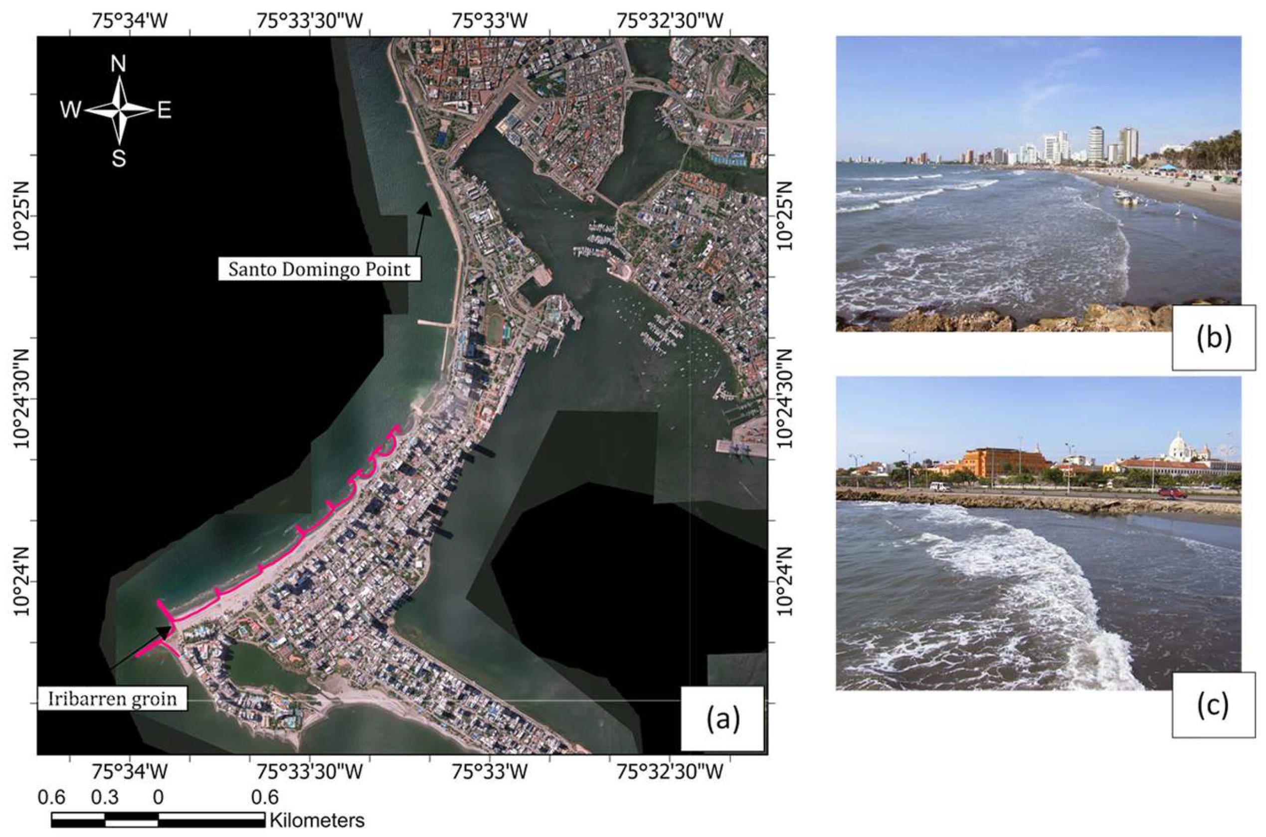
The Bocagrande beach sector spans approximately 1.7 km, extending between 75°34′ W and 75°32′ W, and 10°24′ N and 10°23′ N. It is located on the southern sector of the city and is a bow-shaped bay oriented 40° from North along a NW-SE axis (orthogonal). Two diffraction points constrain it. The northern end diffraction point is a small shoal (Santo Domingo headland) located off a seawall, while the southern diffraction point is an artificially constructed long groin (Iribarren groin) [26]. The indentation ratio (a/Ro = 0.27) and obliquity (β = 24°) classify the site as an exposed, shallow embayment [16,17]. The area is characterized by a flat zone with slight slopes and an elevation near the mean sea level. The entire coastline of this embayment is artificially stabilized. Figure 1a illustrates the location of the case study with a shoreline (pink line) determined during the analysis period (1985–2010). Figure 1b,c show the view from the Iribarren groin and the Santo Domingo point, respectively.

The beach under study is an embayment bounded by a rocky headland to the north and a coastal protection structure to the south. The Bocagrande coastline features various coastal structures, such as groins, breakwaters, and seawalls (dikes), all constructed from limestone quarried close to the city of Cartagena de Indias. In the southern part of the study area, the longest groin, known as the Iribarren Groin, is accompanied by four shorter groins. These are followed by five nearshore breakwaters to the north, with a final groin marking the first section of the beach near the coastline’s curvature. The northern section contains nine short groins, ending at a marginal revetment (seawall) at the other end of the embayment, near the walled city [26].

The tidal regime is mixed, predominantly diurnal (Form Factor F = 1.53), with the lunar declination component K1 exerting the most significant influence on tidal amplitude. The average and maximum mean tides are 0.20 m and 0.55 m, respectively, with a mean tidal range of 0.35 m, indicating a microtidal regime (range < 2 m). Storm surges can raise sea levels by nearly 1.0 m above the normal astronomical tide.

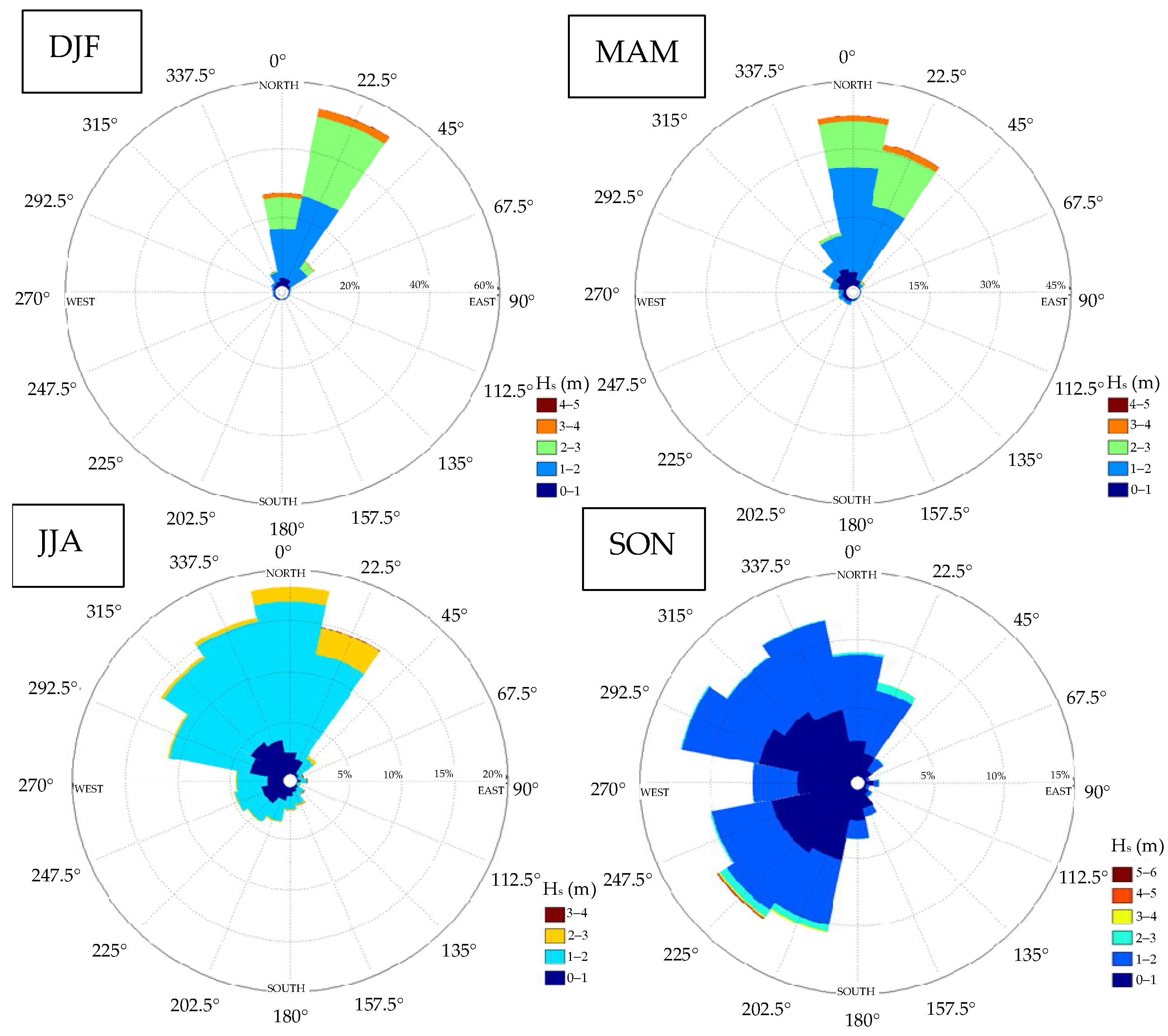
Figure 2 shows the predominant direction of offshore swell in the Colombian Caribbean, indicating that in the December-January-February (DJF) and March-April-May (MAM) quarters, the predominant directions are North (N) and North-Northeast (NNE), which coincide with the presence of the trade winds. For the other two quarters, the directions are more varied. Wave events are grouped into 16 directions with a width of 22.5°. Therefore, when selecting a wave propagation direction for modeling (e.g., N, NNE, NNW), it is assumed that the waves come from the directions shown in the wave rose, with directions ±11.25° represented by a single specific direction.

2.2. Methodology

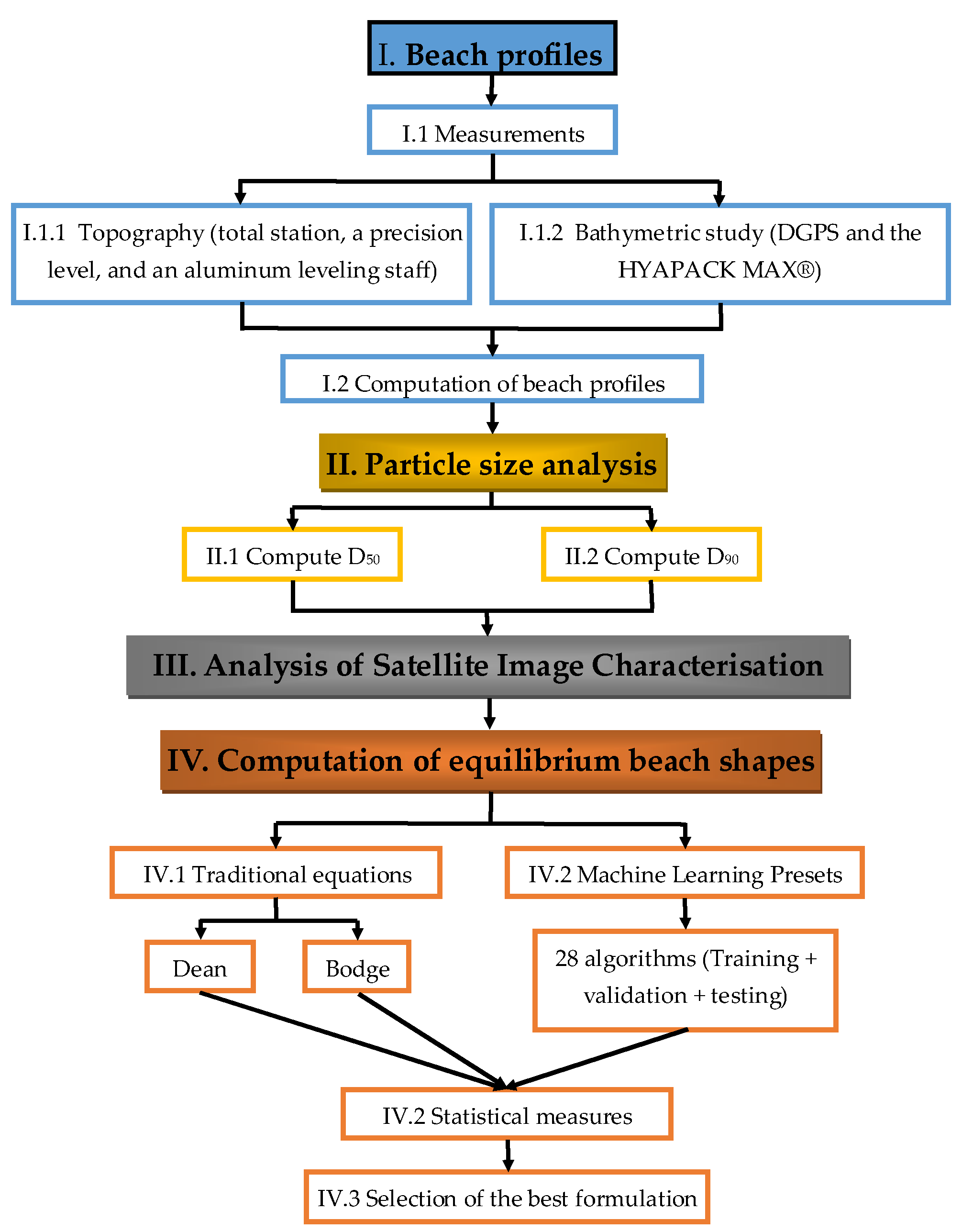
The methodology comprises four stages (beach profiles, particle size analysis, satellite image characterization, and computation of equilibrium beach profiles), as shown in Figure 3.

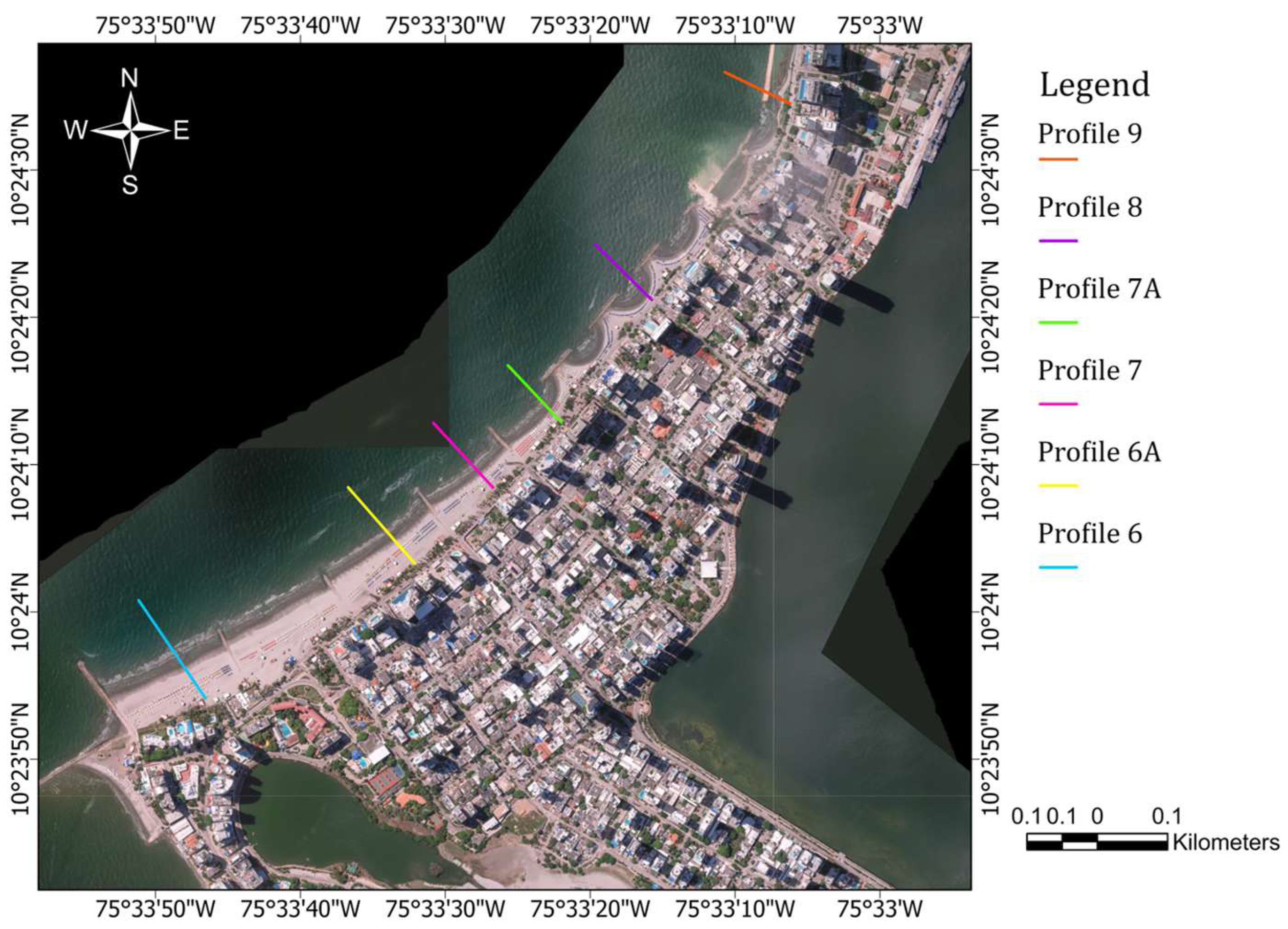
Six beach profiles were measured in the Bocagrande sector from August 2001 to January 2003, June 2007, April and October 2008, in March, May, and June 2012, February to May 2013, March and November 2014, and March to Jun 2016 [27,28,29,30,31,32] (see Figure 4). The profiles in the study area are part of the 34 profiles previously studied by Moreno-Egel et al. [14] designated as 6, 6A, 7, 7A, 8 and 9. Profiles 6, 7, 8, and 9 were installed from 2001 onwards, with the materialized field elements consisting of a concrete cylinder and a metal sheet on the top. Profiles 6A and 7A were installed later in 2012. Dry beach profile data were collected using land surveying techniques (a tachometer and level stations). These profiles extended from the top of the berm to a water depth typically around 1.8 m. Sand samples were taken on the dry beach, at the shoreline, and in the submerged zone to determine the D₅₀ and D₉₀ of the sediment, making a sieve analysis according to the [33]. The sizes of the dry and submerged beaches were averaged. The bathymetric profiles were measured using a boat equipped with integrated DGPS and the HYPACK MAX^® v4.3 (Xylem, Middletown, CT, USA) software and an echo sounder for marine surveying (Odom Hydrotrac II^®, Teledyne Marine, Baton Rouge, LA, USA, 24–340 kHz). The data were corrected for tides and integrated with the topographic measurements of the beach profiles. The accuracy of the bathymetric surveys is estimated at approximately 0.2 m vertically and 0.3 m horizontally.

The shoreline evolution was assessed using aerial photographs from the Instituto Geográfico Agustín Codazzi (IGAC) in Colombia, dating from 1985; orthophotos from 2005; and Google Earth imagery from 2005, 2007, and 2010.

Table 1. Description of the data employed in the shoreline analysis.

Data Type	Year	Resolution	Source
Aerial photographs	1985	15 cm	IGAC
Orthophoto	2005	10–30 cm	IGAC
Satellite imagery	2005	15 cm–15 m	Google Earth Pro
Satellite imagery	2007	15 cm–15 m	Google Earth Pro
Satellite imagery	2010	15 cm–15 m	Google Earth Pro

presents the types of satellite imagery utilized in this study. The base map presented in this study is the 2022 orthophoto of Cartagena de Indias, Colombia, taken by IGAC.

Transects were established at approximately 50-m intervals for the analysis. Once the shorelines had been digitized, a baseline was defined as the reference for evaluating all transects in ArcGIS 10.8.

This data was subsequently compared with the shoreline variations derived from field-measured profiles. Finally, the profiles were fitted to the equilibrium profile formulations proposed by Dean and Bodge.

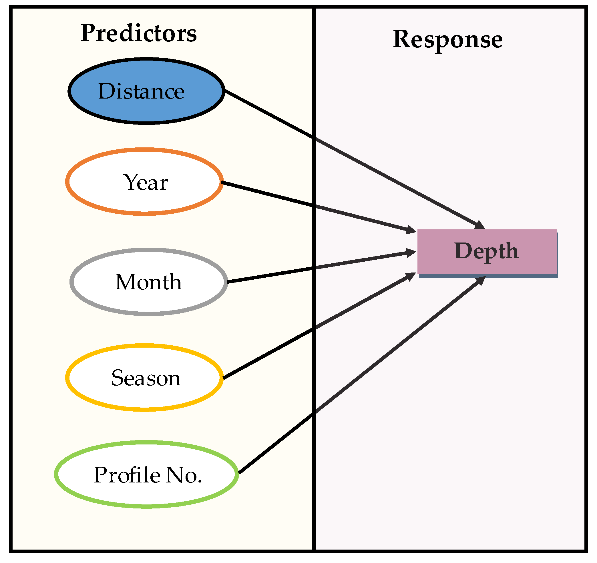
Nine machine learning models were employed to reproduce the beach profiles, simulated using the Regression Learner App in MATLAB, considering not only distance as a predictor but also the year, month, and season in which each profile was measured. Figure 3 presents the methodology used in the study.

Wave approach directions at the breaking zone were measured in the field with a compass during the beach profile surveys. The evolution of the coastline was assessed using aerial photographs from 1985 (IGAC), orthophotos from 2005, orthophoto maps obtained from Google Earth for the years 2005, 2007, and 2010, and coastline surveys from 2001, 2002, 2003, 2008, 2012, 2013, and 2016, which were compared with data obtained from the measured profiles. To define and digitize the coastline on aerial photographs, the point of maximum wave run-up on the dry beach was used, along with the contrast between dry and wet areas.

Beach profiles from different measurement periods were compared to determine the theoretical closure point [34] and to evaluate variations in the width of the dry beach and the longitudinal slope. Variations in beach profiles for the two characteristic climatic periods of the Colombian Caribbean were analyzed to identify possible seasonal variations and assess erosion in the area.

The equilibrium beach shapes were determined and initially adjusted to Dean and Bodge formulations [6,35] giving by Equations (1) and (2), respectively.

$$h\left(x\right)=A{x}^n$$

(1)

$$h\left(x\right)=B\left(1-e^{-kx}\right)$$

(2)

where $h\left(x\right)$ = depth, $x$ = distance, and $A, n, B$, and $k$ are constants that depend on the beach profiles.

Machine learning models were employed to compute the beach profiles [12], considering not only distance as a predictor but also the year, month, and season in which the profile was measured. Figure 5 presents the predictors used and the response variable in this analysis.

In this study, nine types of machine learning models were employed to reproduce the beach profiles, as shown in

Table 2. Model type and presets used for machine learning algorithms.

Model Type	Presets
Linear Regression	Linear, Interactions Linear, and Robust Linear
Stepwise Linear Regression	Stepwise Linear
Tree	Fine, Medium, and Coarse
Support Vector Machine (SVM)	Linear, Quadratic, Cubic, Fine Gaussian, Medium Gaussian, and Coarse Gaussian
Efficient Linear	Least Squares, SVM
Ensemble	Boosted and Bagged Trees
Gaussian Process Regression	Squared Exponential, Matern 5/2, Exponential, and Rational Quadratic
Neural Network	Narrow, Medium, Wide, Bilayered, and Trilayered
Kernel	SVM and Least Squares Regression

, simulated using the Regression Learner App in MATLAB version 2024b [36]. In all cases, a 5-fold cross-validation scheme was applied, with 15% of the data set held out for testing. In total, 649 measured points from the beach profiles were used to train and validate the machine learning models.

During the computations, Gaussian Process Regression (GPR) produced the best results among the machine learning presets. This approach provides a probabilistic framework in which the response function (depth) is assumed to follow a Gaussian distribution, conditioned on the training set ($x_i,y_i$). It is expressed as [37,38]:

$$y=x^T\beta +\epsilon$$

(3)

This probabilistic model is suitable for predicting the depth of a beach profile, $y_{new}$, given new predictors, $x_{new}$, and the data from all beach profiles collected at different times. Here, $\epsilon$ denotes the error variance, while $\beta$ represents the coefficients estimated from the complete dataset.

3. Results and Discussion

The results of wave propagation for the Bocagrande area indicate that waves from the NE, N, and NNE reach heights ranging from 0.6 to 1.2 m in the breaking zone, with values around 0.3 to 0.5 m as the wave trains approach the shoreline. During storm periods with strong wind activity ($H_s$ > 3.5 m), the wave direction near the coast changes to NW-NW, with heights varying from 1.5 to 2.4 m, reaching the breaking zone with heights between 0.5 and 1.2 m. When cold fronts are present in the Caribbean, this significantly affects wave heights ($H_s$ > 4.5 m) [25]. Wave heights near the Bocagrande coast vary between 1.98 and 2.9 m, approaching the breaking zone, where heights range from 1.2 to 1.8 m.

Modal states of the beach were verified for profiles measured in 2007, 2008, 2010, and 2013, and correlated with field data collected in 2016. For waves with $H_s$ less than 1.0 m in the breaking zone, the beach behaves as an intermediate type across all studied profiles, while for waves greater than 1.3 m and periods longer than 7.5 s, it behaves as a dissipative type. For values between these extremes, depending on sediment size in the profile and wave period, both behaviors may be observed in the profiles. The most frequent type of wave breaking is spilling and plunging, depending on the climatic period. On the day of the measurements and deployment of the ADCP current meter (2016), wave heights in the breaking zone ranged from 0.32 to 0.42 m, with periods ranging from 6.8 to 7.8 s, and an average orientation of NW (320°). For these wave heights, the predominant type of breaking was spilling, with Iribarren number values for breaking ranging from 0.2 to 1.0. Regarding the morphodynamic state, the dimensionless fall velocity parameter of grains varied between 1.9 and 2.5, indicating an intermediate state of the beach on the day of the measurements with the current meter.

Sediment size was classified as fine sand according to the Unified Soil Classification System of ASTM, with an average D₅₀ diameter ranging from 0.18 to 0.21 mm, an average mean diameter of 0.20 mm for the entire beach, and a D₉₀ ranging from 0.26 to 0.30 mm. A slight increase in these values was noted compared to data obtained from 2001 and 2002 (D₅₀ = 0.18 to 0.19 mm), which could indicate an increase in the energy received from the waves or the construction of new structures to the north of the beach sector. Sediment sizes varied very little along the beach from south to north of the bay, with a slight increase in size towards the north (see

Table 3. Variation of D₅₀ of measured profiles.

Profile	2001	2002	2007	2008	2012	2013	2016
	D50 (mm)
6	0.18	0.19			0.19	0.20
6A					0.19	0.21
7	0.18	0.18	0.19	0.22	0.20	0.20	0.20
7A					0.19	0.19	0.21
8	0.19	0.20	0.20	0.20			0.22
9	0.19	0.19	0.22	0.21		0.21

).

3.1. Shoreline Variations

The variations in the shoreline across the field-measured profiles were characterized by retreats during the dry season (no rainfall), predominantly driven by the trade winds (N-NE), especially in March and April, followed by recovery of the dry beach width during the rainy months, mainly in August, October, and November. Shoreline variations are presented in Figure 6. However, this pattern does not occur when storms in the Caribbean or cold fronts are present, as observed in the 2013 measurements. For these phenomena, changes are abrupt and occur over a few days. As shown in Figure 7, following the cold front in the first week of March, the greatest shoreline retreats occurred in profiles 6 and 7 in April 2013 (brown bar), with a reduction in dry beach width of approximately 16 m in each profile compared to the measurements from February of the same year being greater in profile 6 further south and less in those located towards the north of the bay. Subsequently, in the following months, the beach recovers if no other meteorological events occur; this is reflected in the May 2016 measurement of profile 7, with a recovery of approximately 5 m.

The widths of the dry beach varied from south to north along the bay, with greater widths towards the south (profile 6), a pattern observed over the years of measurement. The profile with the largest shoreline retreat was profile 8 (15 m in 2016), located between two breakwaters, suggesting that this type of protective structure is another factor influencing shoreline modulation. Over the various years of measurement, the width of the dry beach and consequently the shoreline varied within an average range of 15 m in Profile No. 6, 20 m in Profiles No. 7 and 8, and 10 m in Profile No. 9. These variations correspond with the changes in sediment size along the beach, as indicated in Table 3. The most significant dry beach widths in each profile were recorded between October and November, decreasing from December to reach their lowest values in February and April, before beginning recovery in May. A general trend of shoreline variation was established, with average retreats and advances of 10 to 15 m over the 10 years of measurement, depending on the climatic season and profile location. The variation was minor in profiles towards the southern end of the bay. However, there is a noticeable trend of slower recovery from the periodic erosion processes they experience (Figure 6).

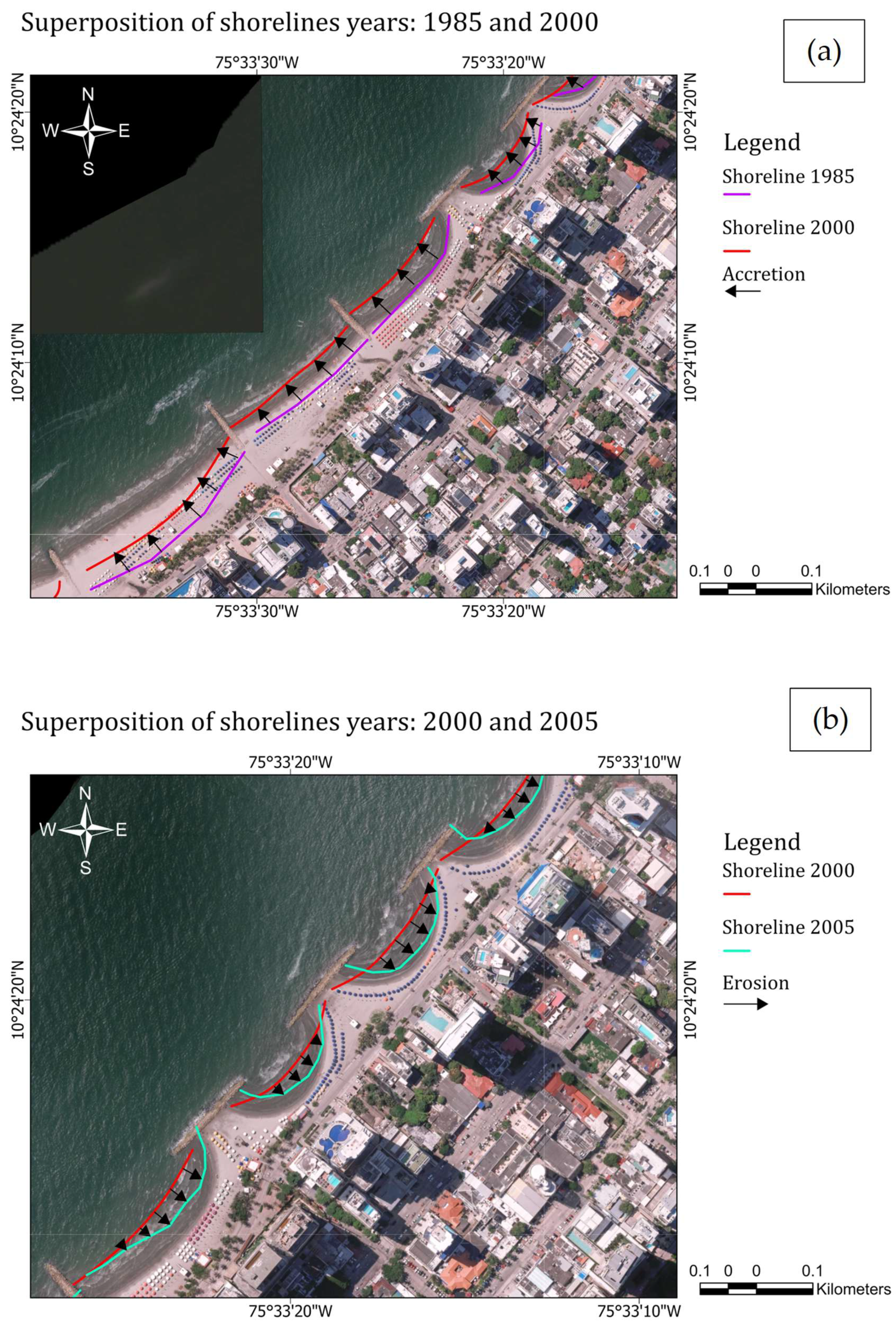
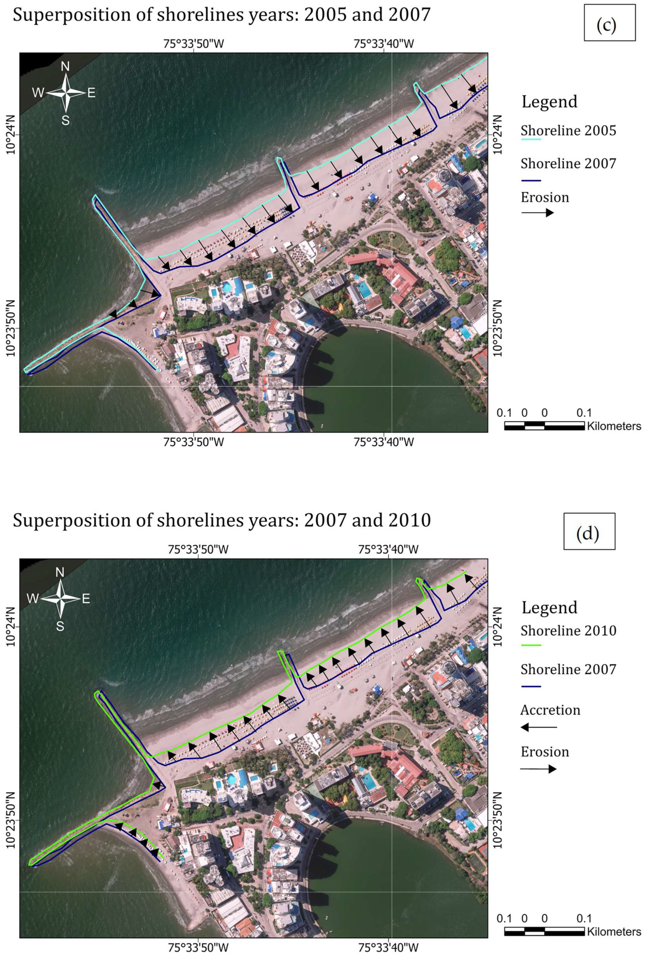
By analyzing the evolution of the shoreline using aerial photographs, orthophotos, and Google Earth images from 1985, 2000, 2005, 2007, and 2010, periodic shoreline retreats and advances are evident, as indicated in Figure 6a–d, with accretion and retreat values ranging from 15 to 22 m. These findings indicate that the Bocagrande beaches experience periodic accretion and erosion processes depending on the time of year and the wave climate conditions [14].

Between 1985 and 2000, accretion predominated, with beach widths ranging from 20 to 22 m (Figure 6a). Between 2000 and 2005, in the area between the breakwater structures, erosion ranged from 19 m to 20 m (Figure 6b). From 2005 to 2007, the area near the Iribarren groyne experienced erosion, with beach width losses of 22–24 m. (Figure 6c). When comparing the shorelines from 2007 and 2010 in the area near the Iribarren groyne, an increase in dry beach width was observed, with shoreline variations of 16–11 m (Figure 6d).

The effects of human intervention on shoreline variation are also evident during the study period. Between 2000 and 2002, construction of protective structures for the Bocana tidal basin in the northern part of the city was completed, along with hydraulic sand filling. In October 2011, the beaches south of Bocagrande were replenished following accelerated erosion near the Iribarren groyne at the end of 2010. In 2016, the protective structures for the depressed road in the Crespo neighborhood, also north of Bocagrande, were completed. These works began in 2013, and marked erosion was observed in the central part of the area, evidenced by shoreline retreat in profile 6, resulting in a loss of nearly 30 m.

3.2. Beach Profile Behavior

When analyzing the dry beach widths for each profile and comparing them with their average longitudinal slopes, no correlation is found between them, as profiles with lower slopes do not show the most significant dry beach widths. Profile No. 6, which has the lowest slope (1.9%), has an average beach width of 78 m, very similar to Profile No. 7 (76 m), which has a steeper slope (3.1%). Similarly, Profile No. 8, which has a gentle slope (2.2%), presents the smallest dry beach width, indicating a greater effect of the profile location along the beach-bay and the type of nearby coastal structures.

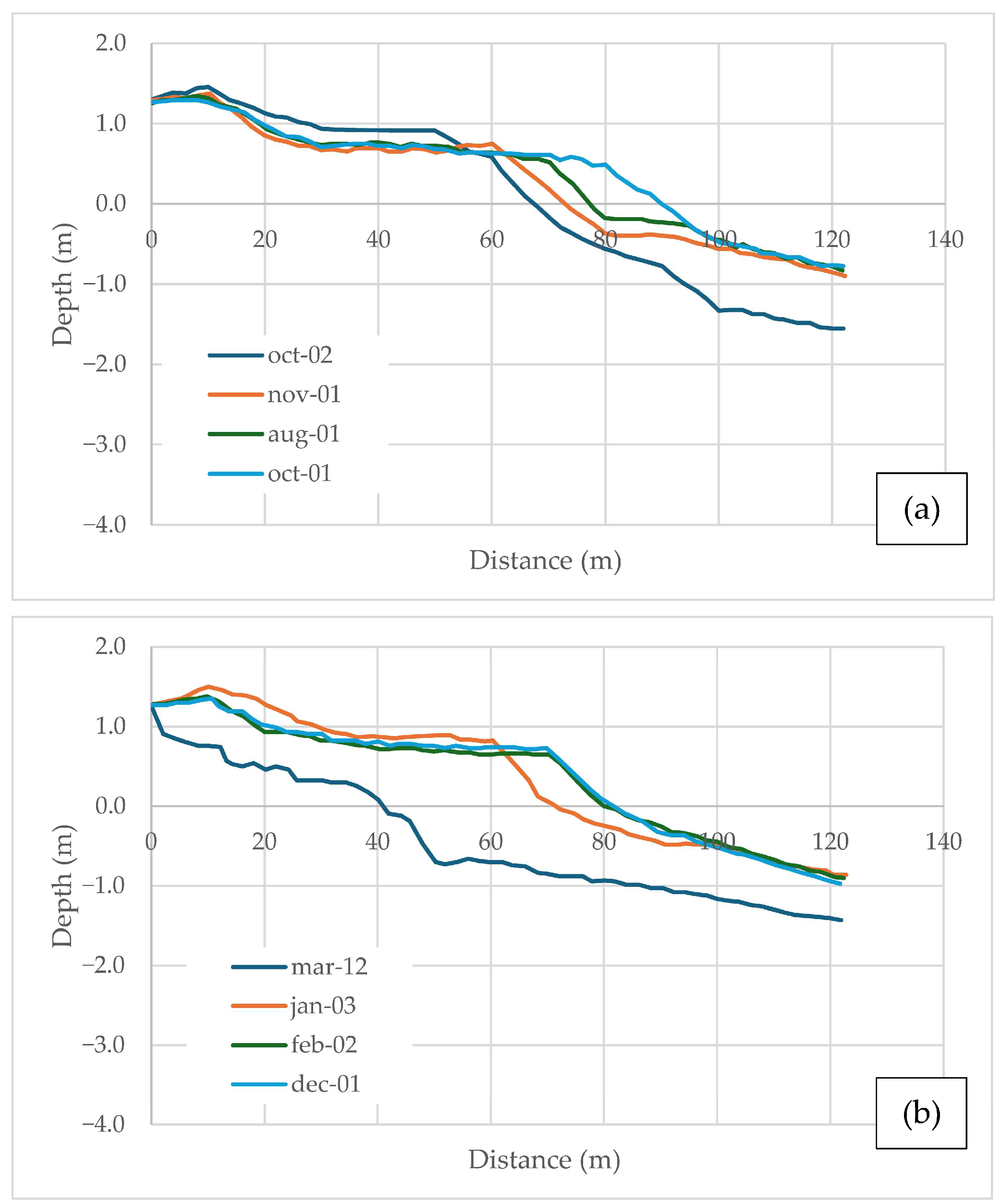
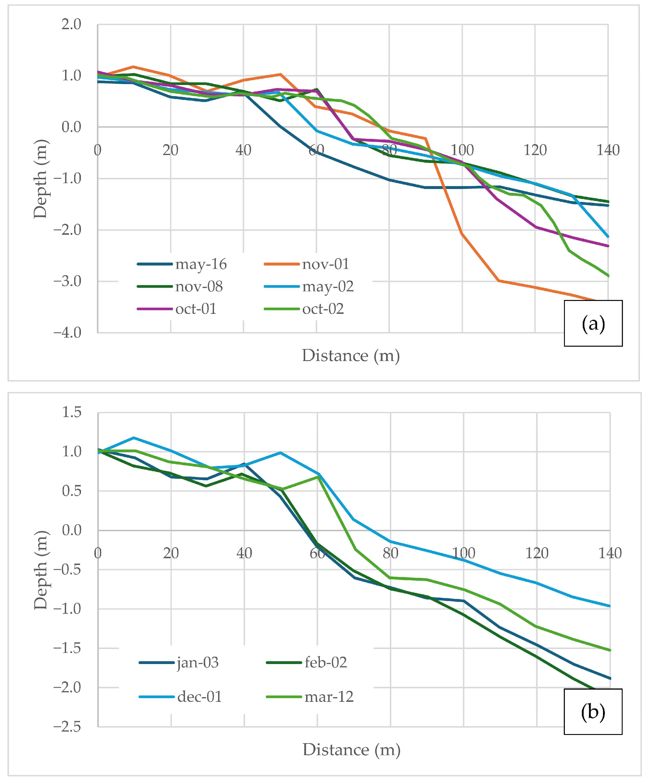
The shapes of the profiles measured across different climatic seasons were also compared to determine whether there were differences. Figure 8 and Figure 9 show the differences between the profiles measured during the rainy and dry seasons for Profiles No. 6 and 7.

The beach profiles exhibited average slopes ranging from 1.9% to 3.8%, with closure depths between 4.0 and 4.5 m for the selected wave conditions. The profile slopes do not follow a uniform pattern from south to north across the bay, seemingly influenced by nearby coastal structures and their positions within Bocagrande Bay. Profile No. 6, located further south and near the Iribarren groin, which is the longest groin, had the lowest slope (1.9%). Profile No. 6A, also between groins, showed the steepest slope (4.2%). Profile No. 7, situated between two shorter groynes, had an average slope lower than the previous one (3.1%). Profile No. 7A, located further north and between a groin and a breakwater, had a lower longitudinal slope (2.2%). Profiles No. 8 and 9, located between breakwaters but further north, had average slopes of 2.2% and 3.8%, respectively, similar to those between groynes in the southern part of the area. The widths of the dry beach along the sector vary from greater to lesser, from south to north, of the bay, with values ranging from 78 to 24 m. The smallest width was recorded in Profile No. 8 (24 m), which was very close to the width of Profile No. 9 (30 m), the northernmost profile.

As shown in Figure 8 and Figure 9, the profiles during the rainy season exhibit steeper slopes in the submerged section, whereas those from the dry season exhibit gentler slopes in the submerged section. This helps dissipate the higher energy waves typical of that climatic period.

An equilibrium profile equation for the beach was estimated by fitting each of the average profiles to the Dean model: $h\left(x\right)=A{x}^{{\displaystyle \frac{2}{3}}}$, with the best fit found for the expression where the value of $A$ is 0.078 and the exponent $n$ is 0.77. This model provided the best fit for 76.5% of the cases, with a higher percentage of accuracy for Profiles No. 6 and 7. However, using Bodge’s equation, a better fit was achieved with a value of $B=4.67$ and a value of $k=7.3\times {10}^{-3}$, showing lower percentage of errors than the adjusted Dean equation, particularly for Profiles No. 8 and 9, indicating once again that the position of the profile within the bay has an impact on its morphodynamic behavior.

The machine learning presets were trained using 28 models, as summarized in Table 4, for Profiles No. 6 and 7. In this analysis, the response variable is depth (in meters), and the predictors include distance (in meters), season (dry or wet), year, month, and profile number (No. 6 or 7). The root mean square error ($RMSE$) and the coefficient of determination (R²) were computed as follows:

For the $RMSE$:

$$\mathrm{R}\mathrm{M}\mathrm{S}\mathrm{E}=\sqrt{{\displaystyle \frac{1}{N}}\sum _{i=1}^N{(h_{T,i}-h_{P,i})}^2}$$

(4)

For the $R^2$:

$$R^2=1-{\displaystyle \frac{\sum _{i=1}^N{(h_{T,i}-h_{P,i})}^2}{\sum _{i=1}^N{(h_{T,i}-\overline{h_T})}^2}}$$

(5)

where $h_{T,i}$ = true value of the depth, $h_{P,i}$ = predicted value of the depth, $h_{P,i}$ = total number of observations, and $\overline{h_T}$ = average value of observations.

Table 4. Results of machine learning presets for Profiles No. 1 and 2.

Preset	$\mathit{R}\mathit{M}\mathit{S}\mathit{E}$ (Validation)	${\mathit{R}}^2$(Validation)	MAE (Validation)	$\mathit{R}\mathit{M}\mathit{S}\mathit{E}$ (Test)	${\mathit{R}}^2$(Test)	MAE (Test)
Linear	0.34	0.86	0.25	0.39	0.84	0.15
Interactions Linear	0.29	0.90	0.22	0.33	0.89	0.11
Robust Linear	0.35	0.85	0.24	0.42	0.82	0.18
Stepwise Linear	0.29	0.90	0.22	0.33	0.89	0.11
Fine Tree	0.28	0.91	0.16	0.35	0.87	0.12
Medium Tree	0.31	0.88	0.21	0.37	0.85	0.14
Coarse Tree	0.41	0.80	0.30	0.46	0.78	0.21
Linear SVM	0.35	0.86	0.24	0.41	0.83	0.17
Quadratic SVM	0.28	0.91	0.20	0.33	0.88	0.11
Cubic SVM	0.32	0.88	0.22	0.25	0.93	0.06
Fine Gaussian SVM	0.21	0.95	0.12	0.24	0.94	0.06
Medium Gaussian SVM	0.22	0.94	0.15	0.27	0.93	0.07
Coarse Gaussian SVM	0.32	0.88	0.21	0.37	0.85	0.14
Efficient Linear Least Squares	0.40	0.81	0.31	0.44	0.80	0.19
Efficient Linear SVM	0.73	0.36	0.51	0.46	0.78	0.21
Boosted Trees	0.25	0.92	0.17	0.31	0.90	0.09
Bagged Trees	0.26	0.92	0.17	0.31	0.90	0.10
Squared Exponential GPR	0.17	0.96	0.08	0.18	0.97	0.03
Matern 5/2 GPR	0.12	0.98	0.06	0.13	0.98	0.02
Exponential GPR	0.11	0.99	0.05	0.17	0.97	0.03
Rational Quadratic GPR	0.11	0.99	0.05	0.15	0.98	0.02
Narrow Neural Network	0.18	0.96	0.13	0.26	0.93	0.07
Medium Neural Network	0.14	0.98	0.08	0.17	0.97	0.03
Wide Neural Network	0.13	0.98	0.07	0.15	0.98	0.02
Bilayered Neural Network	0.15	0.97	0.09	0.20	0.96	0.04
Trilayered Neural Network	0.15	0.97	0.08	0.18	0.97	0.03
SVM Kernel	0.31	0.89	0.17	0.36	0.86	0.13
Least Squares Regression Kernel	0.33	0.87	0.21	0.35	0.87	0.13

Table 4. Results of machine learning presets for Profiles No. 1 and 2.

Preset	$\mathit{R}\mathit{M}\mathit{S}\mathit{E}$ (Validation)	${\mathit{R}}^2$(Validation)	MAE (Validation)	$\mathit{R}\mathit{M}\mathit{S}\mathit{E}$ (Test)	${\mathit{R}}^2$(Test)	MAE (Test)
Linear	0.34	0.86	0.25	0.39	0.84	0.15
Interactions Linear	0.29	0.90	0.22	0.33	0.89	0.11
Robust Linear	0.35	0.85	0.24	0.42	0.82	0.18
Stepwise Linear	0.29	0.90	0.22	0.33	0.89	0.11
Fine Tree	0.28	0.91	0.16	0.35	0.87	0.12
Medium Tree	0.31	0.88	0.21	0.37	0.85	0.14
Coarse Tree	0.41	0.80	0.30	0.46	0.78	0.21
Linear SVM	0.35	0.86	0.24	0.41	0.83	0.17
Quadratic SVM	0.28	0.91	0.20	0.33	0.88	0.11
Cubic SVM	0.32	0.88	0.22	0.25	0.93	0.06
Fine Gaussian SVM	0.21	0.95	0.12	0.24	0.94	0.06
Medium Gaussian SVM	0.22	0.94	0.15	0.27	0.93	0.07
Coarse Gaussian SVM	0.32	0.88	0.21	0.37	0.85	0.14
Efficient Linear Least Squares	0.40	0.81	0.31	0.44	0.80	0.19
Efficient Linear SVM	0.73	0.36	0.51	0.46	0.78	0.21
Boosted Trees	0.25	0.92	0.17	0.31	0.90	0.09
Bagged Trees	0.26	0.92	0.17	0.31	0.90	0.10
Squared Exponential GPR	0.17	0.96	0.08	0.18	0.97	0.03
Matern 5/2 GPR	0.12	0.98	0.06	0.13	0.98	0.02
Exponential GPR	0.11	0.99	0.05	0.17	0.97	0.03
Rational Quadratic GPR	0.11	0.99	0.05	0.15	0.98	0.02
Narrow Neural Network	0.18	0.96	0.13	0.26	0.93	0.07
Medium Neural Network	0.14	0.98	0.08	0.17	0.97	0.03
Wide Neural Network	0.13	0.98	0.07	0.15	0.98	0.02
Bilayered Neural Network	0.15	0.97	0.09	0.20	0.96	0.04
Trilayered Neural Network	0.15	0.97	0.08	0.18	0.97	0.03
SVM Kernel	0.31	0.89	0.17	0.36	0.86	0.13
Least Squares Regression Kernel	0.33	0.87	0.21	0.35	0.87	0.13

According to the results, the Rational Quadratic Gaussian Process Regression (highlighted in grey) achieved the best performance in fitting the beach profile, with $RMSE$ values of 0.11 m and 0.15 m for the validation and testing stages, respectively, and $R^2$ values of 0.99 and 0.98 for the same stages. It is worth emphasizing that this preset provides a more accurate equilibrium beach profile than traditional methodologies (Dean and Bodge), with a best-fit of 0.765.

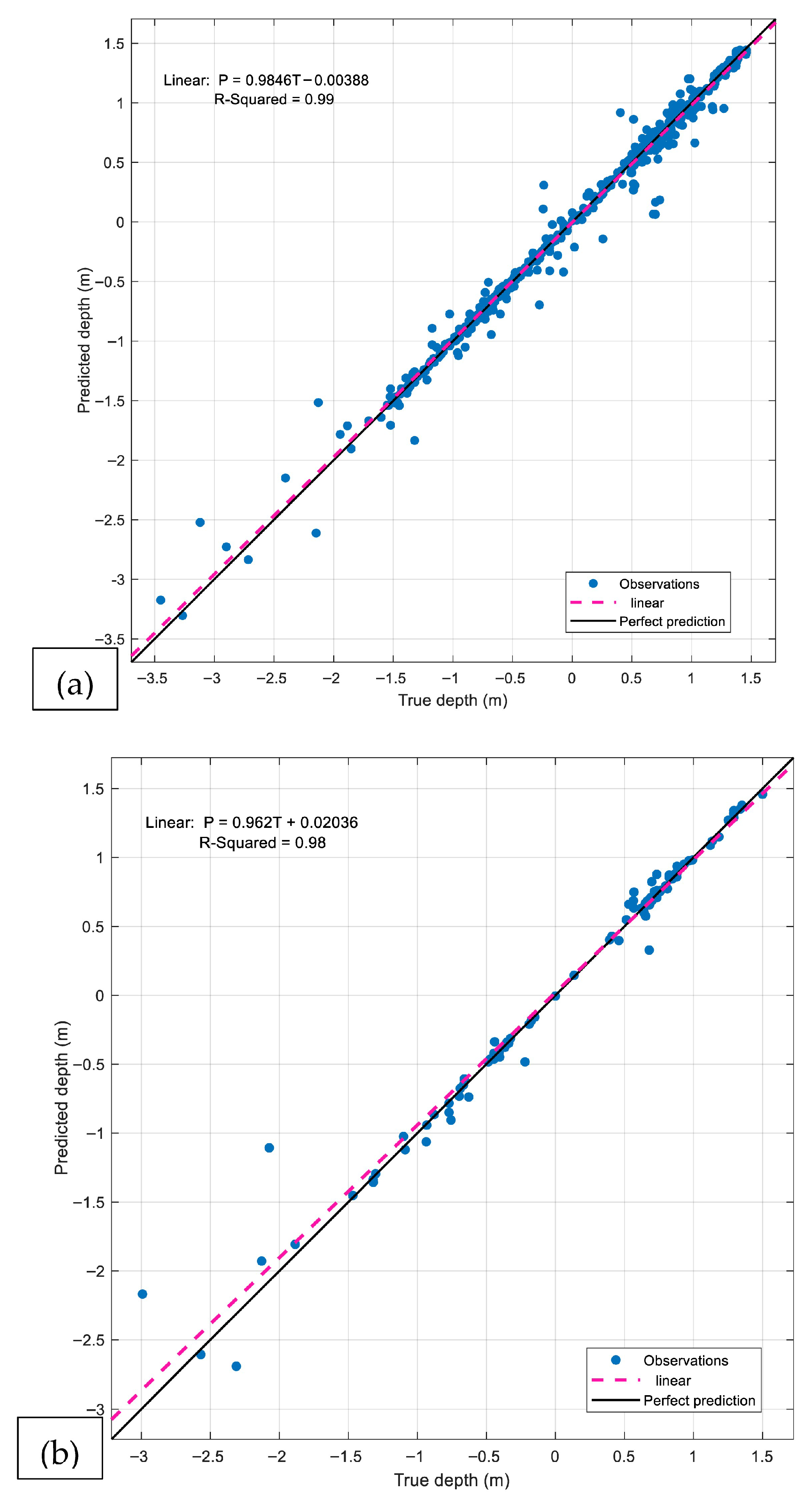
Figure 10 presents all the observations analyzed during the validation and testing stages. The black line represents the perfect fit, while the magenta line corresponds to the predictions obtained with the selected model (Rational Quadratic GPR). Only minor differences are observed between the two lines, reflecting the high model accuracy. The results in both the validation and testing stages confirm the suitability of the selected model, indicating that no overfitting occurred.

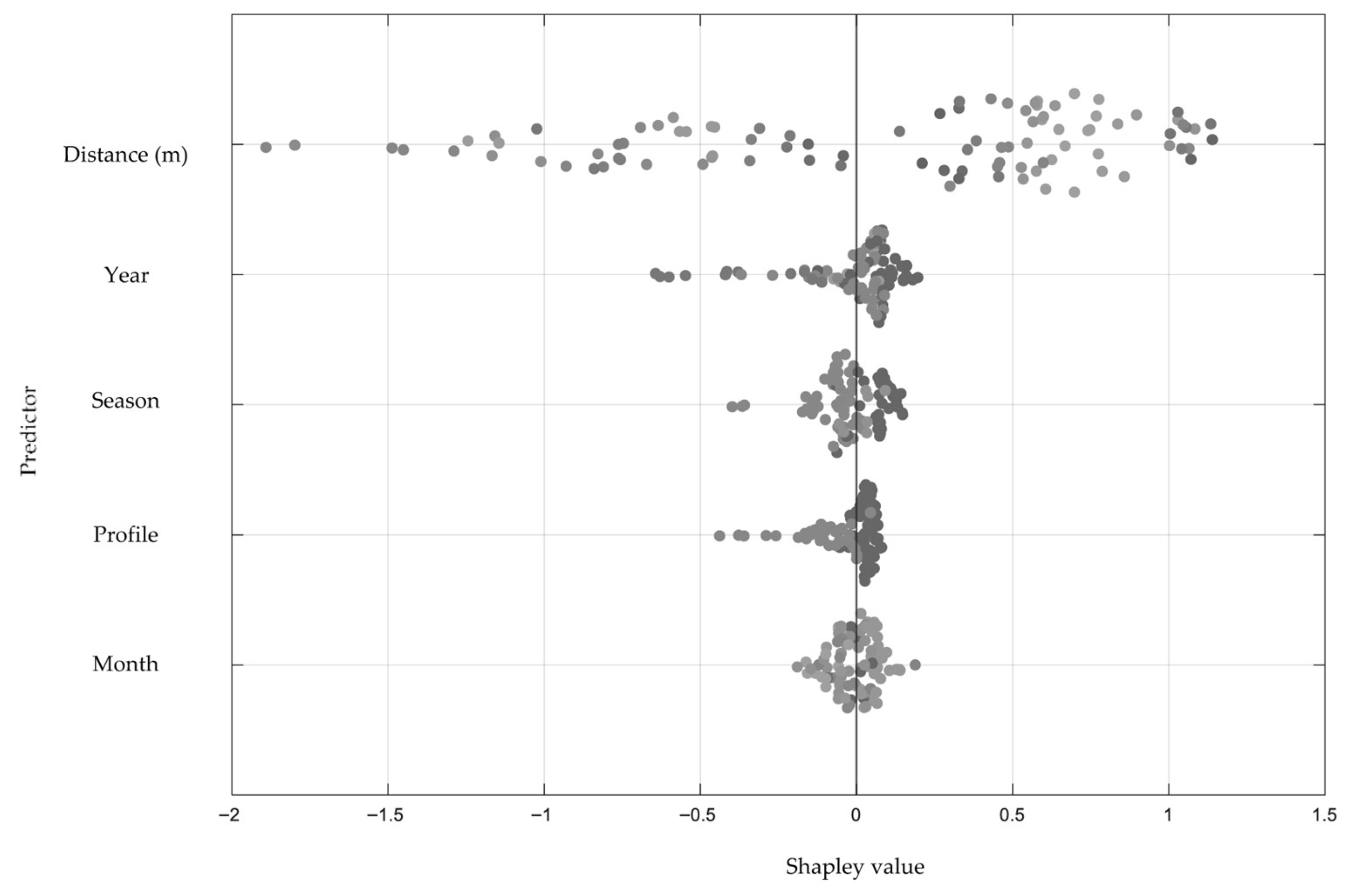
Finally, the Shapley values were computed (see Figure 11) to identify the predictors with the most significant relevance in this study. The results indicate that distance is the most critical factor, consistent with the traditional equilibrium beach profile, while the remaining predictors exert comparatively less influence.

3.3. Discussion

The main beaches facing the Caribbean Sea in the city of Cartagena de Indias, Colombia, share similar morphodynamic characteristics. They have an arched or parabolic shape, with both ends terminating in natural or artificial promontories, and are oriented northeast-southwest. The beaches are classified as microtidal, with relatively shallow inlets. The beaches are dissipative for moderate (>1.0 m) and high (>2.0 m) breaking waves, and intermediate, for low breaking waves (0.3 to 0.9 m high). The predominant direction of the nearby swell, as determined by wave transformation models, is from NNW to NW. The sediments are fine to very fine sand, with an average diameter of less than 0.21 mm. Longshore drift has a predominantly NE-SW direction, producing accumulation on the drifting side upstream of the groins. The direction of sediment transport along the coast can change throughout the year due to storms and cold fronts. For the profiles measured in the field at Bocagrande, the dry beach is wider in the southernmost section of the bay beach, in the most exposed area with the least bay curvature, decreasing in width towards the bay center and increasing again towards the north. Analysis of bay shapes indicates that the beaches are not in static equilibrium [19]. Therefore, any disturbance or interruption in sediment transport causes changes in adjacent bays. For the profiles studied in Bocagrande, the most significant dry beach width occurred at Profile 6 (90 m), at the southernmost part of the bay, and the smallest at Profile 8, towards the center of the bay. During the study, shoreline retreats were recorded due to the construction of new structures north of the bay beach for the profiles analyzed in Bocagrande. During cold fronts, the retreats in Profile 6 were rapid, and the smallest values were observed in Profile 8, although beach recovery was slower. The beach shows a slight tendency towards erosion. The sector along Santander Avenue next to the Bocagrande beaches in the city of Cartagena is situated at position 20 and has been identified as one of the priority areas according to the Master Plan of Coastal Erosion of Colombia [39]. The Coastal Protection Project [26] has been implemented to mitigate coastal erosion problems affecting the city of Cartagena, particularly in the Bocagrande beach zone. Future works must focus on shoreline changes and beach profile behavior, given the Coastal Protection Project under construction in the Bocagrande sector of Cartagena de Indias, Colombia. The current study is an important reference for evaluating future changes to this beach.

4. Conclusions

From monitoring beach profiles in the Bocagrande area, it can be concluded that beach profiles vary over time, both seasonally and with changes in wave climate. For waves with heights less than 1.0 m in the breaker zone, the beach behaves as intermediate across all studied profiles, while for waves exceeding 1.3 m and periods longer than 7.5 s, it behaves as dissipative. The most frequent types of wave breaking are spilling and plunging, depending on the climatic season.

The sediment size was classified as fine sand according to the ASTM Unified Soil Classification System, with an average diameter D₅₀ ranging from 0.19 to 0.21 mm, an average diameter of 0.20 mm for the entire beach, and a D₉₀ between 0.26 and 0.30 mm. A slight increase in these values was observed compared to data from 2001 and 2002.

Shoreline variations in the field-measured profiles were characterized by retreats during the dry season (without rain), with prevailing trade winds (N-NE), especially in March and April, followed by recovery of the dry beach width during the rainy season, mainly in August, October, and November.

The widths of the dry beach varied from south to north in the Bocagrande bay, with greater widths towards the south (Profile No. 6), following the same pattern throughout the years of measurement. The profile with the most incredible shoreline retreats was Profile No. 8 (30 m in 2016).

An average shoreline variation of 10 to 15 m, with retreats and advances, was observed over the 10-year measurement period, depending on the climatic season and profile location. The variation was minor in the profiles towards the southern end of the bay. The study period also highlighted the effects of human intervention on shoreline variation, particularly when new structures were built in the city’s northern part.

The beach profiles exhibited average slopes ranging from 1.9% to 3.8%. Still, they showed no uniform behavior from south to north, seemingly influenced by nearby coastal structures and the profiles’ positions within Bocagrande Bay. There was no correlation between dry beach width and average longitudinal slope: profiles with lower slopes did not have the widest dry beaches.

An equilibrium beach profile equation was estimated by fitting each average profile to the Dean and Bodge models. The Bodge model provided a better fit for Profiles 6 and 7 and also outperformed the Dean model for Profiles 8 and 9. Nevertheless, this study demonstrated that applying machine learning presets substantially improved the fit of the beach profiles, achieving coefficients of determination greater than 0.98.

The profiles indicate that the Bocagrande beaches undergo periodic accretion and erosion, depending on the time of year and wave climate conditions, with variations of 15–20 m. During the dry season, the shoreline retreats, while in the rainy season, recovery begins, though at a slower rate.