Abstract
Recently, different techniques have been proposed for the scheduling and loading problems in cooling plants with chillers in a parallel configuration. Two broad groups can be considered: the online control-based group and the offline optimization-based group. The first group is exemplified by Model Predictive Control, where the selection of control moves provides a solution to both scheduling and loading. The second group includes Optimal Chiller Loading and Optimal Chiller Sequencing algorithms. They usually derive operating plans with some lead time in a batch-like fashion for long horizons. Both groups use forecasts of important factors such as the cooling demand and ambient conditions; hence, they have to deal with inaccuracies in the forecasts. In this paper, a comparison among these two groups is made considering demand uncertainties. The severity of the uncertainty is shown to play a role in the results as well as the controller tuning in the case of the predictive approach. The results are favorable to OCS with respect to overall consumption (up to 15%) but uses more on/off changes in the chiller’s operation (double in some cases).
1. Introduction
Many cooling plants use more than one chiller because the multiple-chiller option allows more flexibility, stand-by capacity and the possibility of maintenance without full stops. Furthermore, under part-load conditions, load sharing can SUPPORT better performance [1].
The operations of multi-chiller plants can be managed in several ways. One group of techniques focuses on how the cooling load demand is split among the installed capacity. These techniques differ in the way that the division is made. Methods in this group range from the simple “load proportional to capacity” scheme to complex optimization methods such as genetic algorithms. Optimal Chiller Loading (OCL) and Optimal Chiller Sequencing (OCS) are examples of this group, where the optimization problem is usually static (i.e., no dynamic effects are considered) [2].
A very different group of techniques relies on ideas from automatic control to drive the real-time operation of the multi-chiller plant. Different control schemes have been proposed for this task, from linear control to model-based nonlinear predictive control [3]. Simple control loops can provide sequencing of chiller units by means of techniques such as total-cooling-load-based control, chilled-water-return temperature-based control, direct-power-based control, and bypass-flow-rate-based control [4]. However, these techniques on their own lack predictive abilities; hence, model-based techniques provide results that are close to optimal for some criteria. In all cases, dynamic models are thus considered to involve the Optimal Control problem. The Optimal Control problem is usually more involved than OCL/OCS problems. As a result, the time spans usually considered by the second group is shorter (minutes, hours) than those of the first (days, weeks). A shorter time span usually brings about sub-optimal results [5,6]. On the other hand, control-based techniques usually consider a set of decision variables much larger than in the first group, potentially providing more degrees of freedom to optimize the plant operation. Furthermore, control-based schemes have the ability to cope with perturbations and uncertainties, in particular those arising from the load demand. In particular, in Model Predictive Control, a moving window provides a future framework where control actions are selected to optimize a function, such as in [3]. Please note that the receding horizon strategy does not (in general) provide a global optimal solution [7,8]. In fact, the optimization problem resulting in these approaches must be solved iteratively using general solvers (nonlinear; non-quadratic).
For the OCS to be undertaken, a model to link control variables to consumption is needed. In most cases, data-sheets from manufacturers are used; in other cases, these data are enhanced with simulations using tools such as TRNSYS [9]. Data-driven approaches have also been proposed in this context [10].
In most of the papers mentioned above, the power load of each chiller in the plant is considered a variable termed the Part Load Ratio (PLR) and used as an independent variable for the optimization problem. However, the PLR is usually not directly controlled during operation; instead, it is a variable resulting from the combination of other variables that can be manipulated, such as mass flows and temperature set points. In addition, the maximum capacity of the chillers has been reported to increase by altering the input and output temperatures of the water in the chiller [11]. These observations have made some researchers to consider other variables as potential opportunities to reduce the power consumption of a cooling plant.
Forecasts of the load demand are used by methods in both groups to anticipate control moves and to optimize operations (e.g., by minimizing consumption). Of course, forecasts are not always 100% accurate; thus, the plans made by OCL/OCS must be adjusted during their execution. Fortunately, multi-chiller plants are usually never driven to full capacity; thus, there is room for real-time changes to be made in cooling production to adequately meet the actual cooling demand. To this end, simple control schemes can be used; optimality, however, is lost to some extent.
From this analysis, it is clear that both groups of techniques for multi-chiller plant operation have some advantages and some drawbacks. This paper carries out a comparison, taking a typical specimen from each group. The scenarios for the comparison are designed to establish a fair ground for both groups. In order to provide a context for the comparison, the next section provides background material for OCL/OCS techniques and for model-based control techniques including bibliographical sources. In Section 3, a description of the main characteristics of the studied cooling plant is presented. Section 4 details the comparison method, including the scenarios and the figures of merit that will be later put in use, and presents the results obtained with each type of technique. The conclusions drawn from the experiments end the paper.
2. Multi-Chiller Plant Operation Schemes
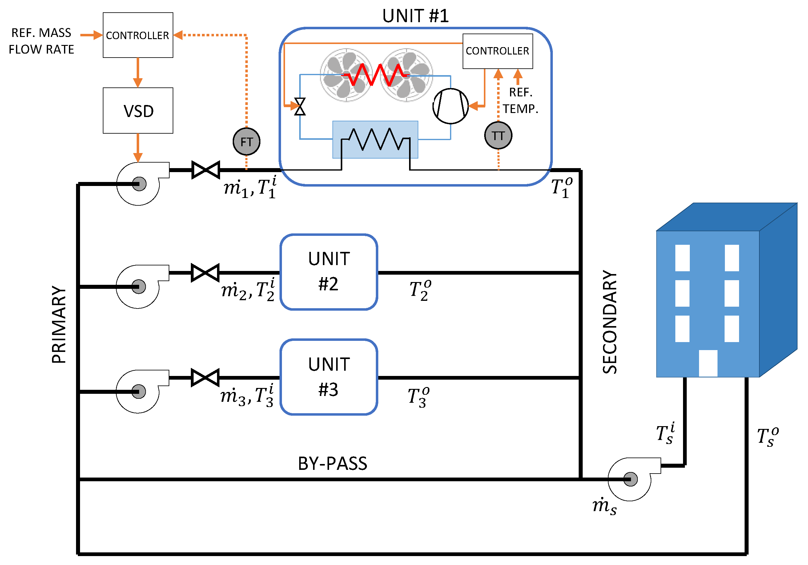
The cooling plant used in this work is constituted by a parallel ensemble of diverse chillers, a bypass pipe and the load, as shown in Figure 1. The function of the bypass pipe is to adapt the primary and secondary mass flow rates. Chiller plant design usually considers peak demand but, in operation conditions, the actual load is most often below the design limit. The load is then partitioned among the chiller units in some way. Optimal Chiller Loading (OCL) considers an economic objective to derive a division of load among units [12]. The variables that are not under control, i.e., disturbances as environment temperature and occupancy level, need to be predicted.
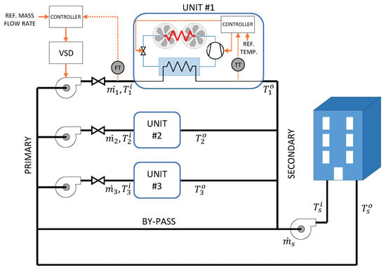
Figure 1.
Diagram of a cooling plant with several chillers serving a building. A detailed view of the low level control loops for the unit #1 is shown.
Different optimization strategies have been proposed to tackle the OCL problem, being specially relevant the case in which the chillers have different characteristics [2]. In the most basic form, OCL does not take into account anything but steady-state relationships and uses the Part Load Ratio (PLR) for each unit as decision variables. As a result, OCL can be solved separately for each time interval considered.
In the Optimal Chiller Sequencing (OCS) problem, a time horizon as a whole must be taken into consideration as a whole: for instance, to contemplate the possible turning on and off of units. The time horizon can range from hours to weeks.
A variety of optimization algorithms have been proposed: for instance, in [13], a genetic algorithm is used for schedule chillers with a non-convex kW-PLR function; in [14], a ripple bee swarm optimization algorithm was selected. Forecasts for cooling demand under uncertainties have been taken into consideration in [15], where different optimization methods are compared. In [16], a electricity tariff rate with hour-wise price variations is included to further reduce costs.
In mathematical terms, the optimization necessary for the OCS problem is an optimal control problem, since it uses a cost functional which is a function of the control variables and the state. For instance, minimum up/down time requirements on the operation of the chillers are considered in [17].
In most of the aforementioned literature, the Part Load Ratio (PLR) is utilized as an independent variable for the optimization problem. However, in practical operation, the PLR is not directly controlled; rather, it results from the combination of other manipulated variables, specifically mass flows and temperature set points.
Furthermore, the maximum capacity of chillers may be improved by altering the evaporator water inlet and outlet temperature as has been reported in [11]. These findings have prompted the consideration of other variables as potential sources for reducing the energy consumption of refrigeration plants, such in [18,19].
The number of active chillers at any given time is separately optimized from their loading in some papers (see [11] and the various references it contains). In this paper, the state (on/off) can be changed during the horizon (unlike in the OCL approach) along with the continuous optimization variables (mass flow rates and temperatures) in a similar manner to the holistic optimization proposed in [20].
In order to link consumption to independent variables, some first principles relationships are used (e.g., conservation laws) together with black-box models: for instance, Coefficient of Performance (COP). For modeling data-sheets from manufacturers, simulations performed with software like TRNSYS (v18) [9] and data-driven approaches [21,22] have been used. Of course, these models and COP estimations must be revalidated from time to time, since the installation might be subject to changes as time passes.
The partition of load among units can also be solved by means of adequate automatic control. A set of control loops can take care of different objectives such as serving the demanded cooling load and maintaining variables within operational limits [23]. These control loops eventually produce a partition of the load, although this can occur in an indirect way. Arguably, the most flexible of the control techniques for this end is model-based control. In model-based control, a model of the plant is used to derive control moves. In particular, the so-called Model Predictive Control (MPC) scheme produces control moves that optimize some objective function for a given time window. This optimal solution is not, in general, a global solution, because the time window (or horizon) cannot be made arbitrarily large.
Both OCS and MPC, are not too far away from each other. Note that OCS does in fact need a model to link decision variables (the PLRs) to consumption. However, the implementation of MPC requires no extra components during the execution phase because it is a control technique. In the case of OCS—which is often not mentioned in the literature—the results obtained from the optimization process must be carried out somehow. During the execution phase, all discrepancies that might occur between plans and actual values must be dealt with. In particular, the cooling load that the plant has to serve is not pre-fixed (in most cases) and one has to resort to forecasts that are not 100% accurate [24]. In fact, the actual total cooling load is dependent on the conditions that the load is served because thermal losses depend on temperature. Recall that OCS relies on chillers output temperature to modulate the power delivery (i.e., to achieve the desired PLRs). Lower water temperatures do, to some extent, increase thermal losses; thus, the total cooling demand also increases.
In order to serve the needed cooling load despite unforeseen conditions, the cooling plant can use simple control loops that take the planned solution as a reference. Low-level controllers can be used to maintain the temperature of chilled water entering the secondary () and the return temperature () within limits.
In the following, the particular OCS to be compared is presented in detail, followed by a similar description for the MPC technique. Table A1 presents a list of the variables and symbols used throughout the rest of the paper. Please notice that the chosen OCS is a state-of-the-art one as it considers more decision variables than just the PLRs as will be commented below. The MPC is also state-of-the art, using a dynamic nonlinear model and a quadratic cost function with constraints. The resulting optimization problem requires some computation time; so, it has been checked that it can be solved withing one sampling period.
2.1. Low-Level Control
The cooling plant relies on low-level controllers for the management of the system. It is necessary to handle the different pumps to control the flows through the pipes of the system, for which it is assumed that necessary measurement elements are available. This control is usually relatively fast (closed-loop dynamics of the order of a few tens of seconds) compared to the time in which the references provided by the optimization layer change (of the order of an hour) to provide temperature and flow rate references to this low-level controllers. According to the work developed in [23], the characteristic time of the controlled temperature at the evaporator outlet is approximately 30 s.
This time length is obtained from the simulation model presented in [23]. The said model is based on the switched moving-boundary approach of Li and Alleyne [25]. There, the heat exchanger is considered as a collection of spatial zones in which the refrigerant appears as superheated vapor or two-phase fluid or subcooled liquid. For medium/large installation the resulting time constant is of the order of 30 s or greater. Now, the longer the transient time the more favorable the setting for the MPC approach will be. This is so because the OCS ignores transients. In order not to bias the results, a lower bound of 30 s is used.
Therefore, taking into account the hierarchy and different time scales of the optimizer and this level of control, in the simulations, it has been considered that the system is already controlled at this level. This will avoid simulating fast dynamics that do not affect the optimization result, and yet it would slow down the execution of simulations.
2.2. OCS Formulation
In OCS, the problem is to determine, for each time period in a given time window (e.g., 24 h), the level of cooling power delivered by each chiller taking into account the on/off switching of units, if needed. The goal is to provide cooling power to meet the load demanded by using the lowest possible electrical consumption. The electrical consumption of each chiller is a function of the evaporator output temperature and the mass flow rate .
In a plant constituted by N chillers, the consumption is defined as
where is the electrical power drawn by chiller i (this includes the power for chiller auxiliary devices), is the electrical power drawn by the secondary pump, is the extra electrical power needed for transients and other effects that will be discussed later and is the sampling period of the time window.
With the definitions given above, the optimization problem is defined in mathematical form for the OCS as
where is a vector of independent variables which contains the trajectories of the variables that define the working point of each chiller i () from to . In mathematical form,
where is the secondary pump mass flow rate. Please note this variable is treated as independent because the presence of a bypass pipe decouples the primary and secondary flow rates.
In Equation (3), the sign denotes a set of points within a trajectory. For a generic variable v, the following definition can be given
The optimization problem defined in (2) is constrained with the following restrictions:
- ensures the cooling power served by the chillers meet the demand and losses for each time period.
- ensures that the decision variables are kept within the bounds required by the installation. This includes minimum and maximum water flow rates, etc.
- is a group of constraints expressed in terms of functions of x. G is a vector function which enables the inclusion of other requirements for the maximum power consumption of each chiller or the allowed range for the water temperature drop in each chiller.
The problem of (2) is a multivariate general optimization problem in which the vector of decision variables has dimension , where N is the number of chillers and T is the number of time steps.
2.3. Model Predictive Control
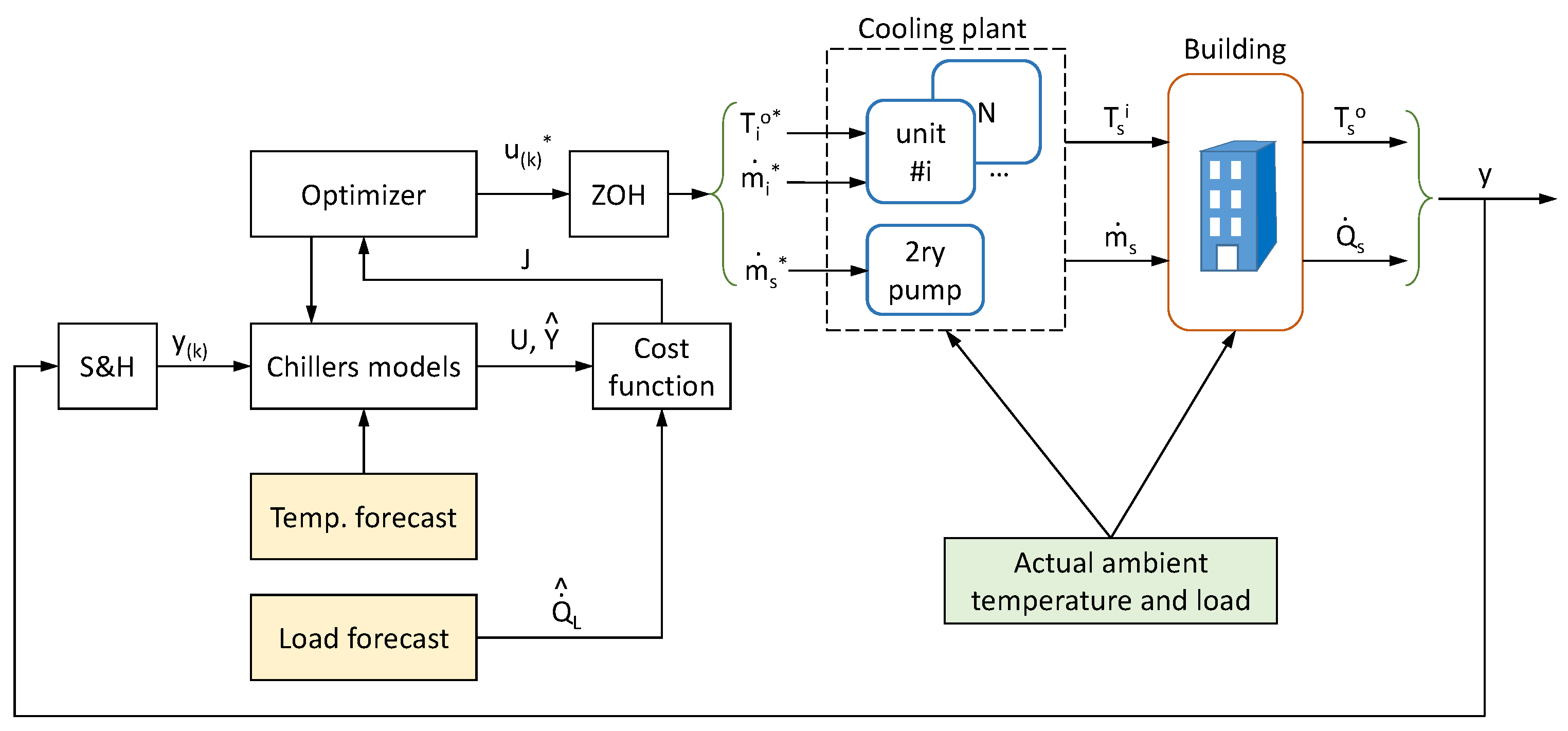
The use of control techniques as opposed to the previous group considered above is motivated by the fact that “Buildings are dynamical systems with several control challenges: large storage capacities, switching aggregates, technical and thermal constraints, and internal and external disturbances (occupancy, ambient temperature, solar radiation)” (quoted from [26]). It is thus natural to include not just automation items but control loops to drive the system towards the objectives, maintaining variables within limits and coping with disturbances. MPC has been applied to building control in many aspects including HVAC management. In [26], the interested reader can find a thorough bibliographical review along with important considerations. As a summary for the particular problem at hand, the following description of MPC can be given with the help of Figure 2, where a typical MPC scheme for use in a multi-chiller cooling plant is presented. The control action u is a vector containing manipulable variables and the sensed variables (such as measured temperatures) are gathered in vector y. The MPC formulation considers a moving time window, spanning from current discrete time k to where H is termed “the horizon”. The control moves are selected by means of an optimization algorithm that aims at minimizing a functional J. This functional typically contains a term penalizing the deviations of from a desired trajectory . The values in the sequence are predictions obtained using the models from the plant fed by U and considering forecasts for variables that cannot be manipulated.
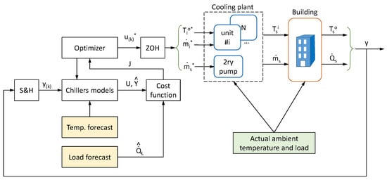
Figure 2.
Diagram of an MPC for a multi-chiller cooling plant.
In many cases, the functional also contains terms used to put a penalty on excessive consumption or other factors. Consumption can typically be related to control moves; so, in many cases, a functional of the following form is used
where is the vector of control action changes. This term is proportional to the consumption associated with changes in the sequence U. The factor is a parameter that allows to put more emphasis on trajectory tracking or consumption penalization.
Minimization of J produces an optimal sequence . Then the receding horizon technique is used, where the first term is delivered to the system as the current control move, discarding the rest of the computed optimal sequence . At the next sampling period the whole procedure is repeated.
The above summary of an MPC is not exhaustive as many options have not been considered. Instead, the presentation has been simplified to fit the purposes of the paper. The important fact to note is that minimization of J does resemble very much the optimization problem of (2). Thus, one might wonder which of the two procedures do actually yield best results.
To ensure a fair comparison, both techniques should be equipped with the same tools; specifically, they utilize identical models for generating predictions and relating decision variables (or control variables in the context of MPC) to energy consumption. In addition to that, the actual MPC formulation that will be used is one of the simplest in order to introduce as few parameters as possible. In this way, the comparison is kept in a fair ground and the tuning of the parameters do not get in the way of the comparison. With this in mind, the MPC optimization problem is described as
which is completely equivalent to (2) except for the temporal span of the involved sequences and for the implementation phase which is trivial in the MPC case but needs some extra components in the OCL/OCS case. Please notice that, in the presence of disturbances of any kind, the MPC formulation ensures a reaction to them if they cause an effect in y. This is possible because MPC is an online algorithm. In the case of OCL/OCS techniques, control loops must be put in place to bring the system back to the desired operating point.
3. Cooling Plant
The methods considered in the paper will be compared using different and realistic profiles for cooling demand and ambient temperature . In all cases the methods are required to fulfill the demand and associated thermal losses maintaining the operational variables within limits.
For the sake of concreteness, a cooling plant with three chillers () is considered in the comparison. The chiller units are commercial air-cooled from TRANE. The manufacturer provides the characteristics shown in Table 1. It can be seen that not only their nominal capacity is different, but also the PLR-kW curves. Please note that the methodology is independent of this choice and can be extended to any number of units with different characteristics.

Table 1.
Main characteristics of the chillers. *1 Cooling power. *2 IPLV values in accordance with ARI Standard 550/590-98 [27].
The rationale for selecting units in a multi-chiller plant are as follows: (1) the installed power must be greater than the maximum expected load, (2) units should have different nominal power so that some are used for situations of low load, others for medium loads and the sum of the units for high loads. In this way, the situation of having to use units at very low load (compared to nominal one) is highly reduced. The machines in Table 1 come from the catalog of a well known vendor and fulfill the previous requisites.
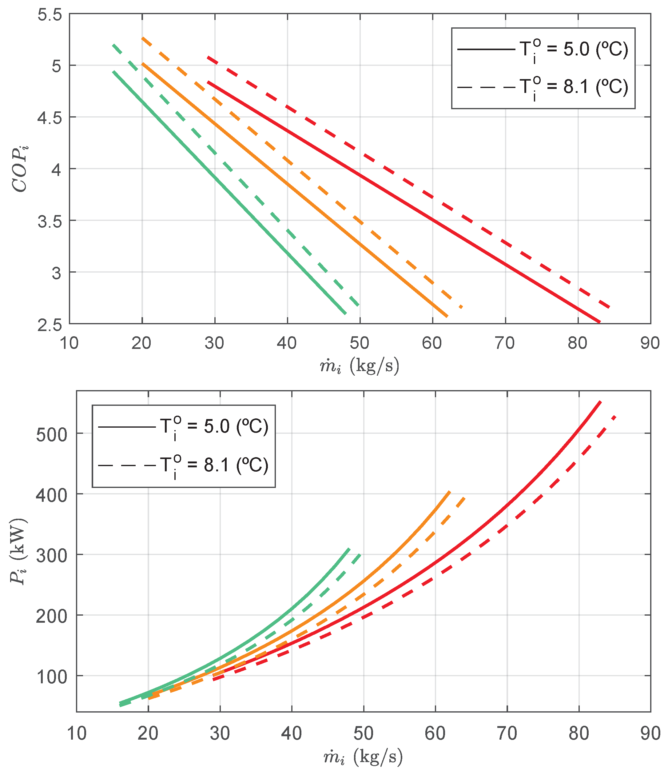
Figure 3 shows the electrical power and COP as functions of the mass flow rate for the chiller models considered in the cooling plant.
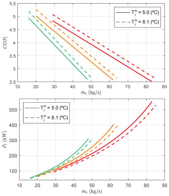
Figure 3.
Electrical power and Coefficient of Performance for a range of mass flows and two output temperatures. Each chiller model is represented in a different color: red for 400 STD, orange for 300 STD, and green for 250 STD.
3.1. Plant Models
The plant models needed by the considered techniques are usually white-box models derived from conservation laws and black-box models to represent COP and other relationships that are more difficult to model using first principles. A survey of models used for control can be found in [23,28]
In the following, the first principles models used for this comparison are defined. First, the cooling provided by the i-th chiller unit in the plant can be expressed as
where is the cooling power (W), is the mass flow rate (kg/s), is the specific heat of water, is the temperature of the water entering the evaporator (K) and is the temperature of the water leaving the evaporator (K). The Part Load Ratio of a chiller is defined as
where is the nominal cooling power of the chiller unit. The Coefficient of Performance of the chiller is obtained from real data provided by the manufacturer. It is a function f of several variables, as follows:
where is the temperature at the evaporator outlet (K), is the temperature at the condenser inlet (K) and is the Part Load Ratio defined earlier. All power consumed by the chiller is included as losses, including ancillary power for the control electronics and fans; so, in this way, it is possible to compute
where (W) is the electrical power drawn by the chiller in order to produce the desired cooling. The temperature of the water entering the secondary can be obtained by the following expression
where is the mass flow rate for the primary defined as
The thermal load due to occupancy (W) and thermal losses (W) produce an increment in the temperature of returned water from the secondary such that the following must hold
In the above equation, is the mass flow rate of water at the secondary (kg/s) which is computed as
where is the mass flow rate that circulates through the bypass. Finally, the temperature can be computed from
Each chiller COP value is interpolated from the corresponding data table provided by the manufacturer to produce function f in Equation (9).
3.2. Integration of Dynamic Effects and Other Losses
In a cooling plant with no thermal storage devices, the most notable dynamic effects are transients produced by the on/off switching of chiller units. Depending on the installation, dynamic effects due to energy storage in the refrigerant inside the chillers, thermal capacitance of the components and refrigerant charge migration can have different time constants.
The dynamical models developed in [25] consider the compressor, the expansion valve and the thermal behavior of secondary fluxes as static due to their faster dynamics compared with other elements. The evaporator and the condenser are modeled using the switched moving-boundary method [29]. From these and similar studies it can be concluded that transients in a chiller can be approximated by low order transfer functions (see the reported results in [30]). The resulting dynamic model can take the form of discrete-time transfer functions [23,31].
The time constants that can be found in the literature for this type of systems are much smaller than the usual time step of one hour established in OCL/OCS problems. This allows for a simplification in the way that transients can be incorporated into the problem. Instead of numerical integration using the transfer function, one just needs to estimate the electrical work needed by the chiller unit to get pass its transient phase. That estimation can then be added up to the other costs for the current hour, namely: electric power for cooling (including thermal losses) and electric power for the secondary pump. This makes sense as any chiller will not add any significant cooling power to the plant until its own state is within the operational limits; so, all work invested in the operation can be counted as losses. In this paper, and considering the characteristics of the chiller units, the time constant is (s); thus, the extra losses are computed, multiplying the set point cooling power by the transient time, which, in a first-order approximation, is estimated as .
This value of is obtained from the chiller on/off operation which corresponds to a fixed operational logic for starting up and shutting down. In particular, the compressor needs some time to start moving due to mechanical inertia, and the fluids need some time to achieve working conditions. This time can be estimated by simple experimentation on the actual chiller unit. It must be noted that, the longer the transient time, the more favorable the setting becomes towards MPC approaches. In order to avoid biases in the comparison, the used value ( (s)) corresponds to a lower bound for the family of chiller units used in the plant.
The power required by the secondary pump operation must be included in the optimization problem. Please note that the secondary pump consumption for different mass flows depends on the characteristic of the installation, in particular in the means used for flow control.
In most OCL works in the literature, the mass flow rates are prefixed; in this paper, they are part of the set of decision variables; thus, the electrical energy consumption of the secondary pump must be taken into account as part of the optimization problem.
Variable-speed pumps are affected by efficiencies that are functions of the rotational speed which depends on the desired flow. Empirical models of electricity consumption for different flows have been constructed from historical data for a particular installation as polynomials of the form [32]:
where .
Please note that interactions between primary and secondary channels could produce changes in flows across the system. However, flows are measured and used in (16); so, the estimation is based on the correct flow. In addition, please note that the flow control loop of the upper left hand corner of Figure 1 ensures that the flows take their correct value through adequate feedback.
Regarding thermal losses, it must be noted that they are dependent on the installation. White-box modeling is possible in principle with the aid of CAD models of the facilities and its thermal insulation. The task can be quite time-consuming and sensitive to parameters that are difficult to measure. However, if the building/installation can be operated with different degrees of occupancy while recording consumption data, it is possible to estimate the amount of cooling load due to occupancy and that due to thermal losses.
To do so, the consumption data can be fitted to models in a variety of ways [33]. In this paper, regression techniques are used. These provide simple models in the form of coefficients for thermal inertia and thermal resistance [34].
Please note that most works consider thermal losses as part of the whole cooling load. In this study, however, the chilled water temperature is considered as a decision variable. As thermal losses depend among other factors on chilled water temperature, the losses must be computed separately.
3.3. Coping with Uncertainties in the Load
Uncertainties on the load can be produced by either measured or unmeasured variables. Ambient temperature is a source of uncertainty that can be measured. Occupancy and thermal processes inside the building are in most cases unmeasured. Disturbances can be considered as ideal measurements affected by uncertainty (white noise, stochastic noise, etc.).
Available disturbances patterns, such as Representative Meteorological Year (RMY), can be used to assess controller performance, although not for actual implementation on a real-time controller as the real disturbance usually has a strong stochastic component. Historical data for a particular building or installation can also be used to provide a more accurate representation of the disturbances [35].
In particular, actual temperature and load profiles can be compared with previous forecasts to identify the distribution of forecast errors. In many cases such distribution is a gaussian or normal distribution. Forecasting methods try to force the mean error to zero and, at the same time, reduce the variance. This is often achieved in average, meaning that for a particular time period (e.g., a day) one might encounter non-zero mean error.
Some papers have dwelt into describing the uncertainty of the load for various energy-related systems. In [36], upper and lower bound estimations are derived using neural-networks. The probability distribution of loads is obtained by means of the singular-value decomposition technique in [37]. Quantile regression neural network models of the load probability have been used in [38] for robust commissioning of cooling plants.
In this paper, the focus is not on obtaining the load uncertainty distribution, but rather to study its effects. To this end, the forecasts of ambient temperature and load are considered affected by uncertainty taking the form of an error distribution following a gaussian with mean and standard deviation .
The real-time application of OCS plans needs some adjustment respect to the planned trajectories. This is so because the actual load and temperature can be different from the forecasts used during the optimization phase. This task can be carried out by low-level controllers that react to excursions of some variables from their reference values. In this way, if the temperature at the secondary circuit is not low enough, the low-level controller would issue an increment in the cooling power issued by the cooling plant; otherwise, the cooling demand would not be satisfied. In this paper, PI controllers are used within each chiller to maintain critical variables within limits, thus ensuring demand satisfaction.
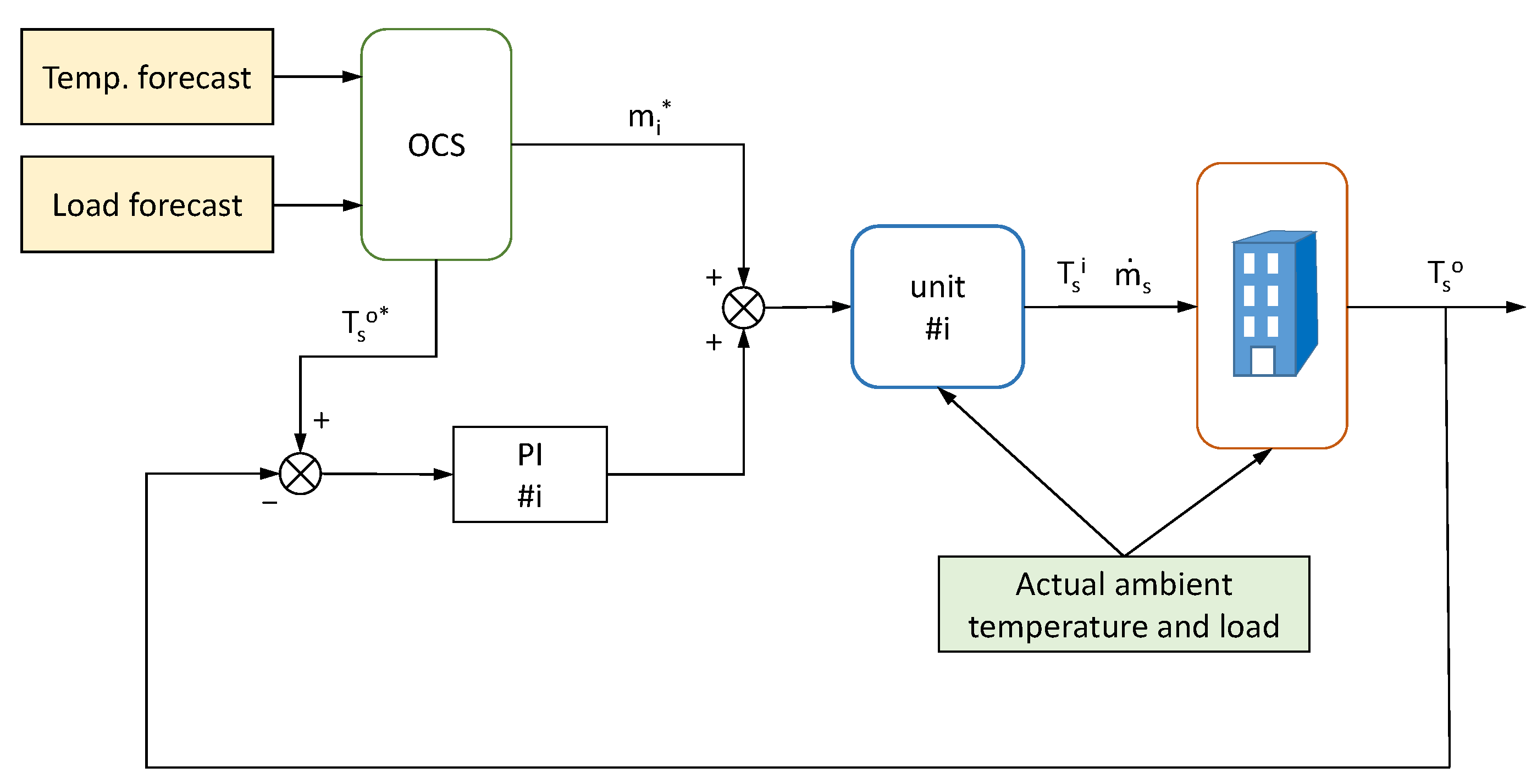
Figure 4 shows a diagram of the control system allowing the OCS plans to be carried out. The output of the offline OCS method dictates the optimal values for and as well as a base value for . The PI controller use and as references and as a feed-forward term. The discrepancies between actual and predicted load causes deviations of temperatures with respect to reference values that the PI can correct acting on the mass flow of the chiller.
where is the feedforward term, is the sampling period, is the proportional gain of the PI and the integral gain.

Figure 4.
Diagram of PI control of chiller mass flow using OCS results as references. Just one chiller is shown for clarity.
In the case of MPC, no extra controllers are needed since it can actually react to changes in the ambient temperature and load with respect to the forecasts thanks to the receding horizon technique. Please notice that the MPC could easily incorporate enhanced forecasts made mid-day, when the actual conditions (temperature and load) are known. This would give an unfair advantage to the MPC scheme and it is avoided in this comparison.
4. Comparison Results
In this section, the results from OCS and MPC control approaches are presented. First, the scenarios characterized by forecast values for ambient temperature and cooling load demand . These forecasts are not 100% accurate; the actual values are the sum of perturbations and the forecasts. In this way, the forecasts can be thought of as base profiles and the perturbations modeled independently.
4.1. Ingredients to Setup Scenarios
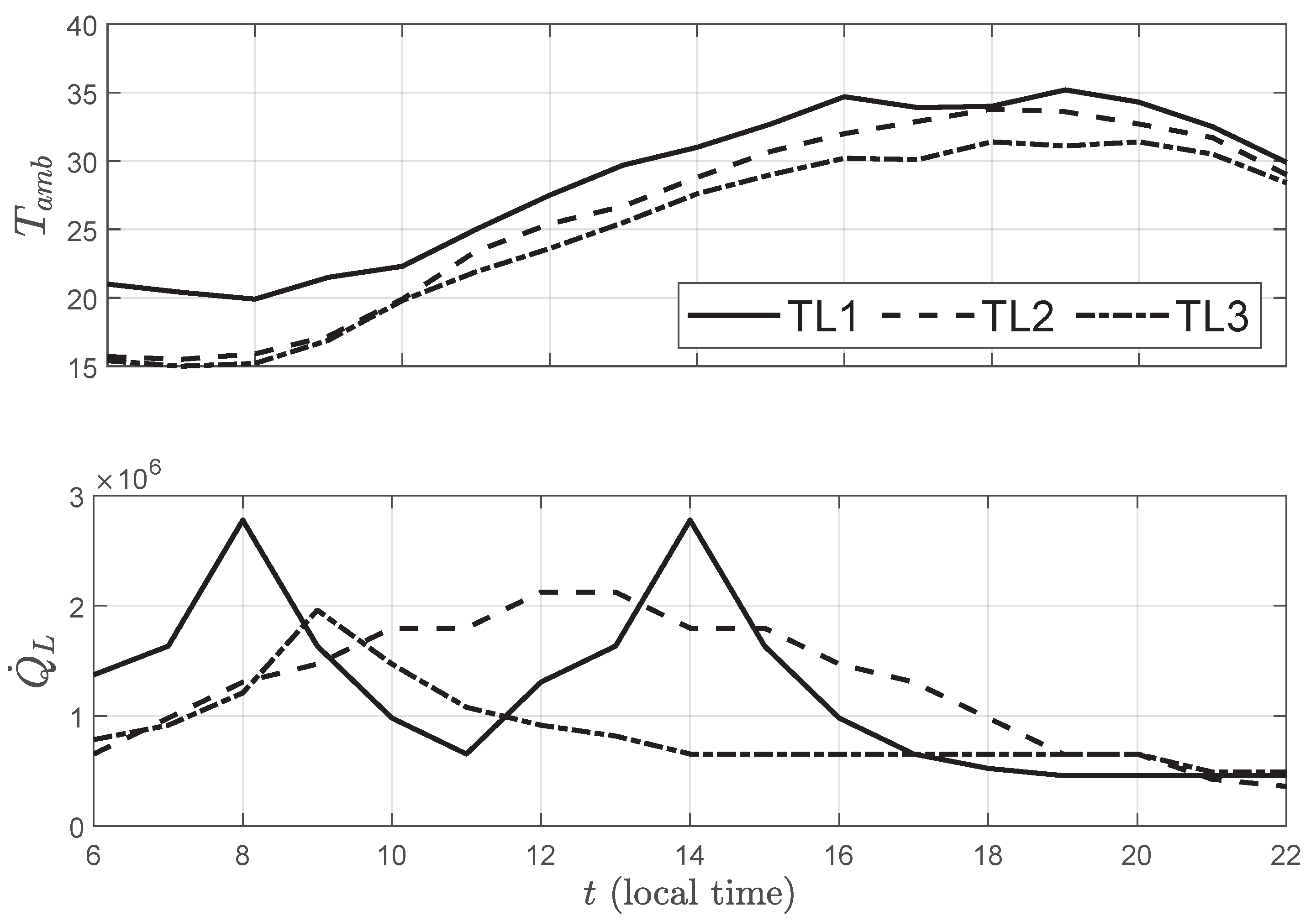
Three different base profiles (TL1, TL2, TL3) will be considered to be used as forecasts for MPC and OCS as shown in the previously presented diagrams of Figure 2 and Figure 4. The profiles correspond to two workdays exhibiting distinct occupancy levels and a half-working day characterized by morning-concentrated usage. Figure 5 presents the trajectories and for the considered base scenarios.
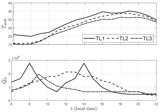
Figure 5.
Forecasts of ambient temperature and load for the considered scenarios.
The actual temperature and load profiles will be obtained adding perturbations to the forecasts. The perturbations are then forecasting errors that will be drawn from a normal distribution that match those observed using usual forecasting techniques [24]. The normal distribution considered for load disturbances is characterized by the mean and the standard deviation . For ambient temperature (°C) and (°C), for cooling load (kW) and (kW).
The final experimental scenarios are a combination of a particular base scenario and a particular perturbation profile and will be discussed in the next Section.
4.2. Results of Chosen Scenarios
The comparison of the two contending techniques will be produced for 9 different cases, C1–C9, where some forecast (base scenario TL1 to TL3) is associated with a particular perturbation profile. The perturbation profile is indicated by and . The cases where no perturbations are added to the forecasts are also included for comparison.
The tuning of the PI used with OCS is . This tuning has been found by extensive trial and error to provide the best possible results. Similarly, the MPC cost function has been subject to a design procedure to find a value for . The best results are found for , although a parameter analysis is included later. Table 2 summarizes the results.

Table 2.
Results for cases C1–C9. Best power consumption cases are indicated in bold.
It is interesting to see that, for cases C1 to C3, the best results are obtained by the MPC method, regardless of the perturbation added. However, for the rest of cases (C4 to C9) the energy consumption of the OCS method is less than that of the MPC method. This is a striking result since MPC incorporates both an optimization method and a way to handle perturbations. One might argue that the particular tuning of the MPC (i.e., cost function design) may play a significant role here. To explore this possibility, Table 3 has been constructed by using different values of with the scenario of case C4. It can be seen that, in general terms, increasing does diminish the number of on/off changes as expected. The total consumption does have a minimum around , but this does not hold for the other cases. Finally, a variable that is very important for the secondary part of the installation is . A low value of means that either is unnecessarily low or that the mass flow is too large. In Table 3, the average value of is given for every tuning. It can be seen that increasing does degrade the value of . This constitutes an additional difficulty for cost function tuning because the obtained value for might not be the same for all cases.

Table 3.
Effect of MPC control effort parameter on the performance of the controller. Best-performing cases per index are indicated in bold.
5. Discussion
The results presented in the previous section showcase the differences in terms of consumption for the two control types. The superiority of one method over the other cannot be established for all possible scenarios. This is an important result for practitioners and for researchers in the field.
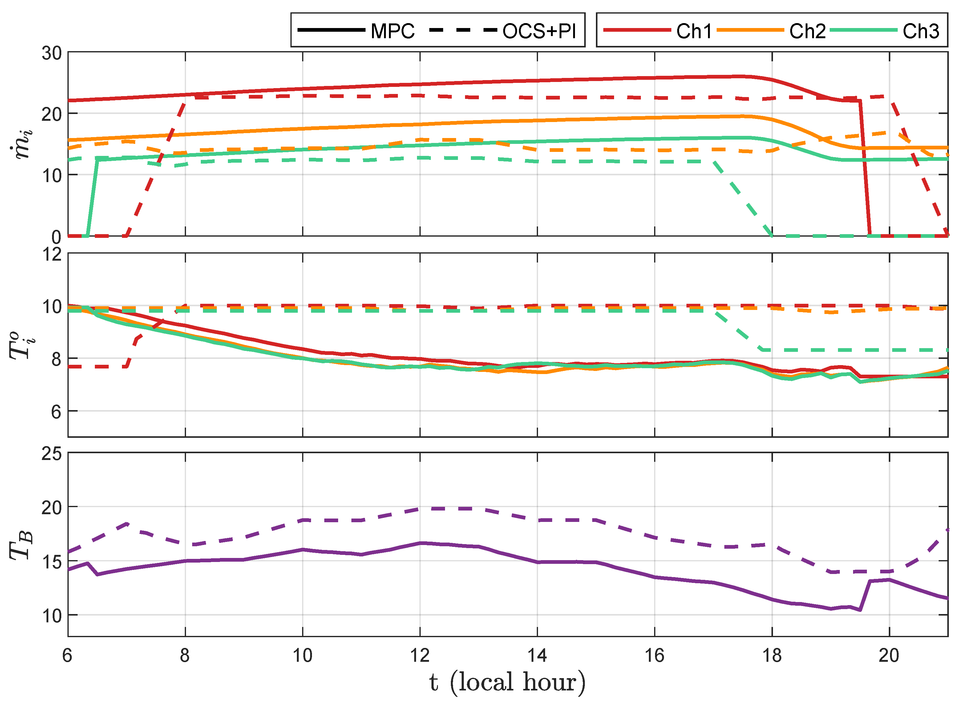
It is also interesting to see how the different methods produce similar trajectories for the variables of interest. In Figure 6, a comparison of results for MPC and OCS is presented considering: mass flows for each chiller (, i = 1, 2, 3), water temperature at the output of each chiller (, i = 1, 2, 3), and water temperature after the bypass, at the secondary entry point (). It is interesting to see that the trajectories are similar, with those of the OCS being less smooth. This is to be expected, since the MPC does include a penalization term for control action changes at each sampling period, whereas the OCS has some freedom during the real-time use of the PI controllers. Of course, a more conservative tuning of the PI can yield smoother trajectories.
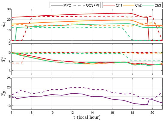
Figure 6.
Trajectories of some variables for chillers in the cooling plant for case C6.
Another important aspect is that of chiller commutations (on-off operations). From Table 2, it is clear that MPC always produce less commutations than OCS. This is important in applications where the number of on-off operations has, not just an immediate economic impact due to losses but also a long-term impact due to maintenance considerations. However, if, during cost function design, it is decided that chiller commutations is not much of an issue, then the MPC method has the capacity to increase this number obtaining some benefits. This can be seen clearly in Table 3. If a value of is chosen, then the overall consumption goes from 34,737 (kWh) to 32,027 (kWh) with a larger value of and with an increase in the number of commutations of 2. This shows one aspect of MPC that makes it an interesting choice: the flexibility. In situations where a compromise (or trade-off) solution must be found, the MPC formulation can be tuned towards one end or the other.
6. Conclusions
This paper presents a comparative analysis of two independently proposed techniques for chiller plant operation. Despite originating from different contexts, their performance proves to be similar. To do so, transients have been considered in the OCS problem in a way that the resulting optimization problem is tractable, the set of decision variables have been extended with respect to previous OCS approaches, and forecasts uncertainties are parametrized to yield different scenarios for comparison. While the results are slightly more favorable to OCS regarding overall consumption, Model Predictive Control (MPC) offers distinct advantages. Specifically, MPC eliminates the need for additional tunable controllers and provides flexibility through the parameter to to shift the solution towards different objectives. Moreover, MPC can easily incorporate updated intra-day forecasts as actual temperature and load conditions become known.
Author Contributions
Conceptualization, M.G.S. and M.R.A.; methodology, M.R.A.; software, M.G.S. and J.M.M.-H.; validation, M.G.S., A.P.V.-L. and J.M.M.-H.; formal analysis, M.G.S. and M.R.A.; investigation, M.G.S.; resources, M.R.A.; data curation, A.P.V.-L. and J.M.M.-H.; writing—original draft preparation, M.G.S. and M.R.A.; writing—review and editing, A.P.V.-L., J.M.M.-H. and M.R.A.; visualization, M.G.S.; supervision, M.R.A.; project administration, M.R.A.; funding acquisition, M.R.A. All authors have read and agreed to the published version of the manuscript.
Funding
This research received no external funding.
Institutional Review Board Statement
Not applicable.
Informed Consent Statement
Not applicable.
Data Availability Statement
Dataset available on request from the authors.
Conflicts of Interest
The authors declare no conflicts of interest.
Abbreviations
The following abbreviations are used in this manuscript:
| CAD | Computer-Aided Design |
| IPLV | Integrated Part Load Value |
| OCL | Optimal Chiller Loading |
| OCS | Optimal Chiller Sequencing |
| SPSA | Simultaneous Perturbation Stochastic Approximation |
Appendix A
Table A1 presents a list of the variables and symbols used throughout the paper in alphabetical order.

Table A1.
List of used variables and symbols.
Table A1.
List of used variables and symbols.
| Variables | Meaning and Units |
|---|---|
| Specific heat of water (W kg−1 K−1) | |
| Coefficient of Performance | |
| J | Jacobian of objective function |
| Mass flow rate (kg s−1) | |
| Thermal power (W) | |
| T | Temperature (K) |
| P | Electrical power (W) |
| Part Load Ratio (pu) | |
| Vector of independent variables | |
| Subscripts | Meaning |
| amb | Ambient |
| b | Bypass |
| i | Chiller number |
| j | Iteration |
| k | Index to elements in |
| l | Thermal losses |
| L | Load |
| o | Occupancy |
| p | Primary |
| s | Secondary |
| Superscripts | Meaning |
| Condenser | |
| Evaporator | |
| i | Input |
| o | Output |
| n | Nominal |
| Quantities | Meaning |
| N | Number of chiller units |
| Number of commutations | |
| T | Number of time instants |
References
- Dossat, R.J. Principles of Refrigeration; John Wiley & Son: Hoboken, NJ, USA, 1961. [Google Scholar]
- Salari, E.; Askarzadeh, A. A new solution for loading optimization of multi-chiller systems by general algebraic modeling system. Appl. Therm. Eng. 2015, 84, 429–436. [Google Scholar] [CrossRef]
- Candanedo, J.; Dehkordi, V.; Stylianou, M. Model-based predictive control of an ice storage device in a building cooling system. Appl. Energy 2013, 111, 1032–1045. [Google Scholar] [CrossRef]
- Wang, S. Intelligent Buildings and Building Automation; Routledge: Oxfordshire, UK, 2009. [Google Scholar]
- Colodro, F.; Torralba, A. Multirate single-bit Sigma Delta modulators. IEEE Trans. Circuits Syst. II Analog. Digit. Signal Process. 2003, 49, 629–634. [Google Scholar] [CrossRef]
- Deng, K.; Sun, Y.; Li, S.; Lu, Y.; Brouwer, J.; Mehta, P.G.; Zhou, M.; Chakraborty, A. Model Predictive Control of central chiller plant with thermal energy storage via dynamic programming and mixed-integer linear programming. IEEE Trans. Autom. Sci. Eng. 2014, 12, 565–579. [Google Scholar] [CrossRef]
- Bordons, C.; Ruiz, M.; Camacho, E.F.; Tejera, J.M. Energy saving in a copper smelter by means of model predictive control. In Identification and Control: The Gap Between Theory and Practice; Springer: Berlin/Heidelberg, Germany, 2007; pp. 63–85. [Google Scholar]
- Chinde, V.; Woldekidan, K. Model predictive control for optimal dispatch of chillers and thermal energy storage tank in airports. Energy Build. 2024, 311, 114120. [Google Scholar] [CrossRef]
- Wang, L.; Lee, E.W.; Yuen, R.K. A practical approach to chiller plants’ optimisation. Energy Build. 2018, 169, 332–343. [Google Scholar] [CrossRef]
- Castilla, M.d.M.; Campoy-Iniesta, C.; Álvarez, J.D. Reinforcement Learning based Thermal Comfort Control in buildings. RIAI 2025, 22, 140–145. [Google Scholar]
- Huang, S.; Zuo, W.; Sohn, M.D. Amelioration of the cooling load based chiller sequencing control. Appl. Energy 2016, 168, 204–215. [Google Scholar] [CrossRef]
- Chang, Y.C. A novel energy conservation method—Optimal chiller loading. Electr. Power Syst. Res. 2004, 69, 221–226. [Google Scholar] [CrossRef]
- Chang, Y.C. Genetic algorithm based optimal chiller loading for energy conservation. Appl. Therm. Eng. 2005, 25, 2800–2815. [Google Scholar] [CrossRef]
- Lo, C.C.; Tsai, S.H.; Lin, B.S. Economic dispatch of chiller plant by improved ripple bee swarm optimization algorithm for saving energy. Appl. Therm. Eng. 2016, 100, 1140–1148. [Google Scholar] [CrossRef]
- Saeedi, M.; Moradi, M.; Hosseini, M.; Emamifar, A.; Ghadimi, N. Robust optimization based optimal chiller loading under cooling demand uncertainty. Appl. Therm. Eng. 2019, 148, 1081–1091. [Google Scholar] [CrossRef]
- Shao, Z.; Gholamalizadeh, E.; Boghosian, A.; Askarian, B.; Liu, Z. The chiller’s electricity consumption simulation by considering the demand response program in power system. Appl. Therm. Eng. 2019, 149, 1114–1124. [Google Scholar] [CrossRef]
- Acerbi, F.; Rampazzo, M.; Nicolao, G.D. An Exact Algorithm for the Optimal Chiller Loading Problem and Its Application to the Optimal Chiller Sequencing Problem. Energies 2020, 13, 6372. [Google Scholar] [CrossRef]
- Thangavelu, S.R.; Myat, A.; Khambadkone, A. Energy optimization methodology of multi-chiller plant in commercial buildings. Energy 2017, 123, 64–76. [Google Scholar] [CrossRef]
- Chiam, Z.; Easwaran, A.; Mouquet, D.; Fazlollahi, S.; Millás, J.V. A hierarchical framework for holistic optimization of the operations of district cooling systems. Appl. Energy 2019, 239, 23–40. [Google Scholar] [CrossRef]
- Karami, M.; Wang, L. Particle Swarm optimization for control operation of an all-variable speed water-cooled chiller plant. Appl. Therm. Eng. 2018, 130, 962–978. [Google Scholar] [CrossRef]
- Sala-Cardoso, E.; Delgado-Prieto, M.; Kampouropoulos, K.; Romeral, L. Predictive chiller operation: A data-driven loading and scheduling approach. Energy Build. 2020, 208, 109639. [Google Scholar] [CrossRef]
- Ho, W.; Yu, F. Variable importance for chiller system optimization and sustainability. Eng. Optim. 2021, 54, 504–523. [Google Scholar] [CrossRef]
- Bejarano, G.; Alfaya, J.A.; Rodríguez, D.; Morilla, F.; Ortega, M.G. Benchmark for PID control of refrigeration systems based on vapour compression. IFAC-PapersOnLine 2018, 51, 497–502. [Google Scholar] [CrossRef]
- Arahal, M.R.; Ortega, M.G.; Satué, M.G. Chiller Load Forecasting Using Hyper–Gaussian Nets. Energies 2021, 14, 3479. [Google Scholar] [CrossRef]
- Li, B.; Alleyne, A.G. A dynamic model of a vapor compression cycle with shut-down and start-up operations. Int. J. Refrig. 2010, 33, 538–552. [Google Scholar] [CrossRef]
- Killian, M.; Kozek, M. Ten questions concerning model predictive control for energy efficient buildings. Build. Environ. 2016, 105, 403–412. [Google Scholar] [CrossRef]
- ARI Standard 550/590-98; Standard for Water Chilling Packages Using the Vapor Compression Cycle. Air-Conditioning and Refrigeration Institute: Arlington, VA, USA, 1998.
- Li, X.; Wen, J. Review of building energy modeling for control and operation. Renew. Sustain. Energy Rev. 2014, 37, 517–537. [Google Scholar] [CrossRef]
- Grald, E.W.; MacArthur, J.W. A moving-boundary formulation for modeling time-dependent two-phase flows. Int. J. Heat Fluid Flow 1992, 13, 266–272. [Google Scholar] [CrossRef]
- Lei, Z.; Zaheeruddin, M. Dynamic simulation and analysis of a water chiller refrigeration system. Appl. Therm. Eng. 2005, 25, 2258–2271. [Google Scholar] [CrossRef]
- Romero, J.; Navarro-Esbrí, J.; Belman-Flores, J. A simplified black-box model oriented to chilled water temperature control in a variable speed vapour compression system. Appl. Therm. Eng. 2011, 31, 329–335. [Google Scholar] [CrossRef]
- Lu, L.; Cai, W.; Soh, Y.C.; Xie, L.; Li, S. HVAC system optimization—Condenser water loop. Energy Convers. Manag. 2004, 45, 613–630. [Google Scholar] [CrossRef]
- Pokorska-Silva, I.; Kadela, M.; Orlik-Kożdoń, B.; Fedorowicz, L. Calculation of building heat losses through slab-on-ground structures based on soil temperature measured in situ. Energies 2021, 15, 114. [Google Scholar] [CrossRef]
- Gabbar, H.A.; Bondarenko, D.; Hussain, S.; Musharavati, F.; Pokharel, S. Building thermal energy modeling with loss minimization. Simul. Model. Pract. Theory 2014, 49, 110–121. [Google Scholar] [CrossRef]
- Colodro, F.; Torralba, A.; Laguna, M. Time-interleaved multirate sigma-delta modulators. In Proceedings of the 2005 IEEE International Symposium on Circuits and Systems, Kobe, Japan, 23–26 May 2005; pp. 5581–5584. [Google Scholar]
- Quan, H.; Srinivasan, D.; Khosravi, A. Uncertainty handling using neural network-based prediction intervals for electrical load forecasting. Energy 2014, 73, 916–925. [Google Scholar] [CrossRef]
- Khoshrou, A.; Pauwels, E.J. Short-term scenario-based probabilistic load forecasting: A data-driven approach. Appl. Energy 2019, 238, 1258–1268. [Google Scholar] [CrossRef]
- Ding, Y.; Su, H.; Liu, K.; Wang, Q. Robust commissioning strategy for existing building cooling system based on quantification of load uncertainty. Energy Build. 2020, 225, 110295. [Google Scholar] [CrossRef]
Disclaimer/Publisher’s Note: The statements, opinions and data contained in all publications are solely those of the individual author(s) and contributor(s) and not of MDPI and/or the editor(s). MDPI and/or the editor(s) disclaim responsibility for any injury to people or property resulting from any ideas, methods, instructions or products referred to in the content. |
© 2026 by the authors. Licensee MDPI, Basel, Switzerland. This article is an open access article distributed under the terms and conditions of the Creative Commons Attribution (CC BY) license.

