Abstract
This study investigates the influence of stratification—the vertical layering of particles with different sizes—on porosity in granular sediment packings. Conventional porosity models are typically formulated for homogeneous, well-mixed grain assemblies; however, natural riverbed sediments often exhibit stratification, leading to deviations from these idealized conditions. Part I established empirical relationships describing transition layer geometry and porosity in systems composed of low-friction glass beads. Building on this foundation, Part II extends the analysis by incorporating the higher inter-particle friction characteristic of natural sediments, using discrete element method (DEM) simulations to quantify its effect on packing structure and porosity. A refined method is used to extract porosity and density distributions from simulated packings, enabling accurate identification of transition layers. Empirical formulas are developed to predict key transition-layer parameters (thickness, average porosity, and minimum porosity) as functions of the grain-size ratio. A density-based porosity prediction model is introduced and coupled with an existing model for well-mixed sediments, allowing for a quantitative comparison between stratified and homogeneous packing scenarios. Results show that stratification can increase porosity by 44–57% relative to well-mixed samples of an identical grain-size composition. These findings highlight the importance of considering sediment stratification when modeling riverbed porosity and pave the way for improved sediment transport and hydraulic predictions.
1. Introduction
Porosity, defined as the ratio of void space to total volume in a granular medium, is a fundamental physical property of sedimentary deposits. It influences the initiation of sediment motion and the bed level change [,,,,,,,,,], hydraulic conductivity [], storage capacity [], and ecological functions of sediment beds [,], and it plays a critical role in various geotechnical processes [,]. Stratification—a widespread phenomenon in natural fluvial systems—refers to the vertical layering of sediments resulting from variable depositional conditions [] (pp. 76–79). Unlike well-mixed sediments, stratified deposits exhibit complex, inhomogeneous internal structures where fine particles may not effectively fill the voids between coarser grains. This structural inhomogeneity can significantly alter the porosity distribution and, by extension, the behavior and functionality of the sediment bed. Understanding porosity in such stratified systems is therefore essential for accurately characterizing natural sediments and modeling their mechanical and hydraulic behavior.
In the first part of this two-part study, the porosity distribution within stratified granular samples was investigated using a combination of laboratory experiments and DEM-based numerical simulations. A non-destructive experimental setup was introduced to measure the vertical porosity profile of samples composed of glass beads. The DEM software Particula 1.3 [] was then calibrated and validated against the experimental data. However, both experimental and numerical investigations in Part I relied exclusively on glass beads with smooth surfaces, which differ from natural sediments that typically have irregular, rough surfaces and higher inter-particle friction. Since the main objective of this study is to understand the porosity behavior of natural riverbed sediments, it becomes essential to examine how increased inter-particle friction—more representative of real sediment—affects the formation and extent of the transition layer between sediment strata.
This study hypothesizes that the formation of the transition layer is closely linked to the “bridging effect”, a phenomenon where small particles are prevented from infiltrating deeper into the base layer due to the formation of stable interlocking structures across pore spaces [,,,,]. High inter-particle friction is expected to promote the stability of these bridges, thereby inhibiting infiltration and limiting the depth of the transition layer. To test this hypothesis, the validated DEM model in Part I is applied here to simulate stratified packing using friction parameters representative of natural sediments. These simulations allow for detailed analysis of infiltration patterns under high-friction conditions and provide insight into how friction influences porosity structure in stratified deposits.
As established in Part I, a stratified sample can be conceptually divided into homogeneous layers, where porosity is relatively constant and known (typically between 0.36 and 0.4), and inhomogeneous transition layers, where porosity varies due to grain interpenetration. Accurately determining the length and porosity of each transition layer is thus a prerequisite for predicting the average porosity of a stratified sample (Figure 1):
Figure 1.
Sketch of a stratified sediment packing.
Here, and represent the length of the i-th transition layer and the average porosity of the layer, respectively.
In this second part of the study, a predictive model is proposed to estimate the density distribution of infiltrating particles based on the grain-size ratio between layers. This model is used to compute the average porosity of the transition layers and, consequently, the overall porosity of the stratified structure. The empirical model is then coupled with the well-established Yu & Standish model [,] for predicting porosity in well-mixed grain mixtures. Through this coupling, the porosity difference between stratified and uniformly mixed sediments of identical composition can be quantitatively assessed.
The remainder of this paper is structured as follows: In Section 2, the setup and results of the numerical simulations conducted using high-friction particles are presented. In Section 3, the development of the predictive model for infiltration density curves and the empirical model for estimating average porosity in stratified samples is described. The accuracy of the proposed models is also evaluated in Section 3. Finally, in Section 4, the limitations and implications of the empirical model introduced in this study are discussed.
Porosity Predictor of Yu & Standish for Well-Mixed Grain Packings
The Yu & Standish model [,] is an analytical approach to predict the porosity of particulate mixtures based on their size distribution. Initially formulated using laboratory data for binary (two-fraction) mixtures, the model describes porosity through a piecewise-linear relationship between the specific volume Vtot = 1/(1 − porosity) and the volume fraction X. The mixture porosity is defined by the maximum of two linear relations between Vtot and X.
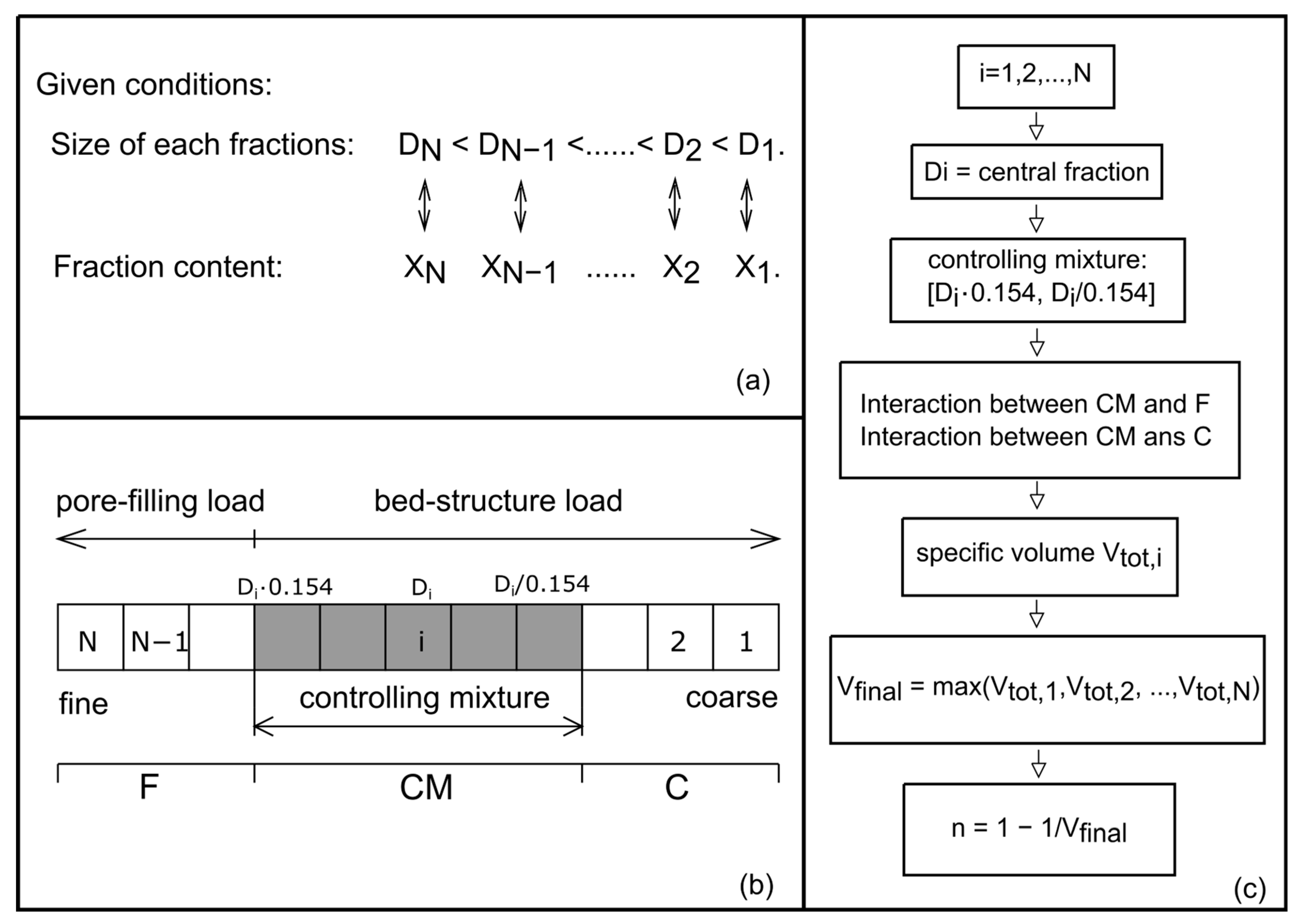
Building on this concept, Yu & Standish [,] extended their model to multi-fraction mixtures by assuming that a linear relationship between Vtot and X also holds for these more complex systems. Central to their method is the idea of a controlling mixture, which includes a central fraction with a representative particle size Di, and the coarsest and finest fractions at sizes Di/0.154 and Di⋅0.154, respectively (Figure 2a,b). Here, 0.154 corresponds to the size ratio between fine and coarse grains to allow the fine grains to pass through the pores built by coarse grains in a tetrahedral packing []. Particles finer than Di⋅0.154 are assumed to act as pore-filling particles, meaning they occupy the voids of the controlling mixture without altering its structural framework.
Figure 2.
(a) Required given conditions to apply the Yu and Standish predictor (b) Definition of the boundary size between pore-filling load and bed-structure load according to [,], and (c) calculation flow sheet of the analytical predictor of Yu and Standish [,]. Figure adapted from [].
To apply the model, each fraction in a mixture is temporarily treated as the central fraction Di of a potential controlling mixture. The specific volume Vtot is then calculated for each scenario, considering interactions between finer (pore-filling) and coarser (structure-forming) particles. The maximum computed Vtot identifies the densest possible packing and delivers the predicted porosity n = 1 − 1/Vtot (Figure 2c).
This model provides a valuable framework for understanding and predicting packing behavior in granular mixtures, especially in systems with wide particle size distributions. A more comprehensive description of the model is available in [].
2. Numerical Simulation
Using the validated DEM software Particula [] introduced in Part I, the influence of increased inter-particle friction—more representative of real sediment—on the formation and extent of the transition layer between sediment strata is examined.
The numerical framework of Particula 1.3—including contact detection, impulse-based contact resolution, and time-step integration—was described in detail in Part I. Briefly, Particula resolves particle interactions using continuous collision detection [] and an impulse-based solver [,] that enforces momentum conservation and frictional constraints at contact points. The relative velocities at contact are used to compute normal and tangential impulses, ensuring non-penetration and adherence to Coulomb friction limits. Particle velocities and positions are updated using a semi-implicit Euler integration scheme, which enhances numerical stability under stiff contact conditions and large time steps [].
2.1. Methodology
2.1.1. Simulation Setup
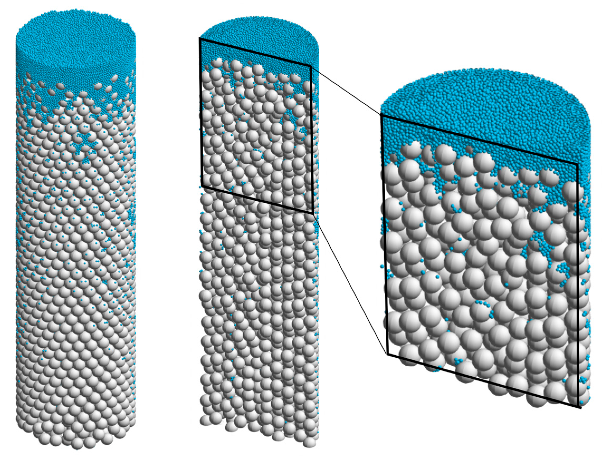
In the numerical simulations, stratified samples were generated by sequentially depositing spherical particles of different sizes into a cylindrical container (Figure 3). During deposition, particles fell freely under gravity, and their motion—including collisions with other particles and the container walls—was fully resolved. To promote denser packing at the base, vibrations were applied during the deposition of the base-layer particles; this vibration was disabled during the deposition of the top layer.
Figure 3.
Examples of stratified samples generated by numerical simulation with bottom layer 21 mm and top layer 3.5 mm.
The simulation software Particula 1.3 supports two boundary condition types: hard boundaries and soft boundaries, implemented by defining a buffer zone. The buffer zone refers to a peripheral region near the model boundary where particle deposition is prohibited. When the buffer zone length is set to zero, particles directly contact the container wall, leading to increased porosity within a region of approximately 5 grain diameters due to the “Wall Effect” []. In contrast, when the buffer zone is greater than zero, particles are prevented from contacting the container boundary, effectively mimicking a soft boundary condition in which particles can partially pass through an imaginary wall. This significantly reduces the influence of wall effects on the sediment structure.
In this study, soft boundary conditions were employed. To improve the relevance of the findings to natural sedimentary environments, the simulations incorporated the friction and restitution coefficients representative of natural sediments. Effect of these material properties on the key characteristics of the transition layer was evaluated: its dimensionless thickness φT (φT = LTransition_Layer/DBase, where DBase represents the diameter of the base-layer-particles), the average porosity nm and the minimum porosity nmin within the transition layer. Additionally, the critical value of R′ corresponding to the onset of unlimited percolation of upper-layer particles was explored.
Following the generation of samples with a 20 cm diameter under soft boundary conditions, the central 10 cm core of each sample was extracted for analysis to eliminate regions affected by boundary influences. For each simulation condition, two repetitions were performed to ensure reproducibility.
The simulation parameters are summarized in Table 1. In the numerical simulations, a total of 34 different combinations of top- and base-layer grain size ratios, denoted as R, were investigated, where R = DTop/DBase. Here, DTop represents the grain size of the top sediment layer, and DBase represents that of the base layer. All combination cases are summarized in Appendix A. As noted in Part 1, this study primarily focuses on cases where DBase is larger than DTop.
Table 1.
Simulation parameters.
2.1.2. Data Analysis
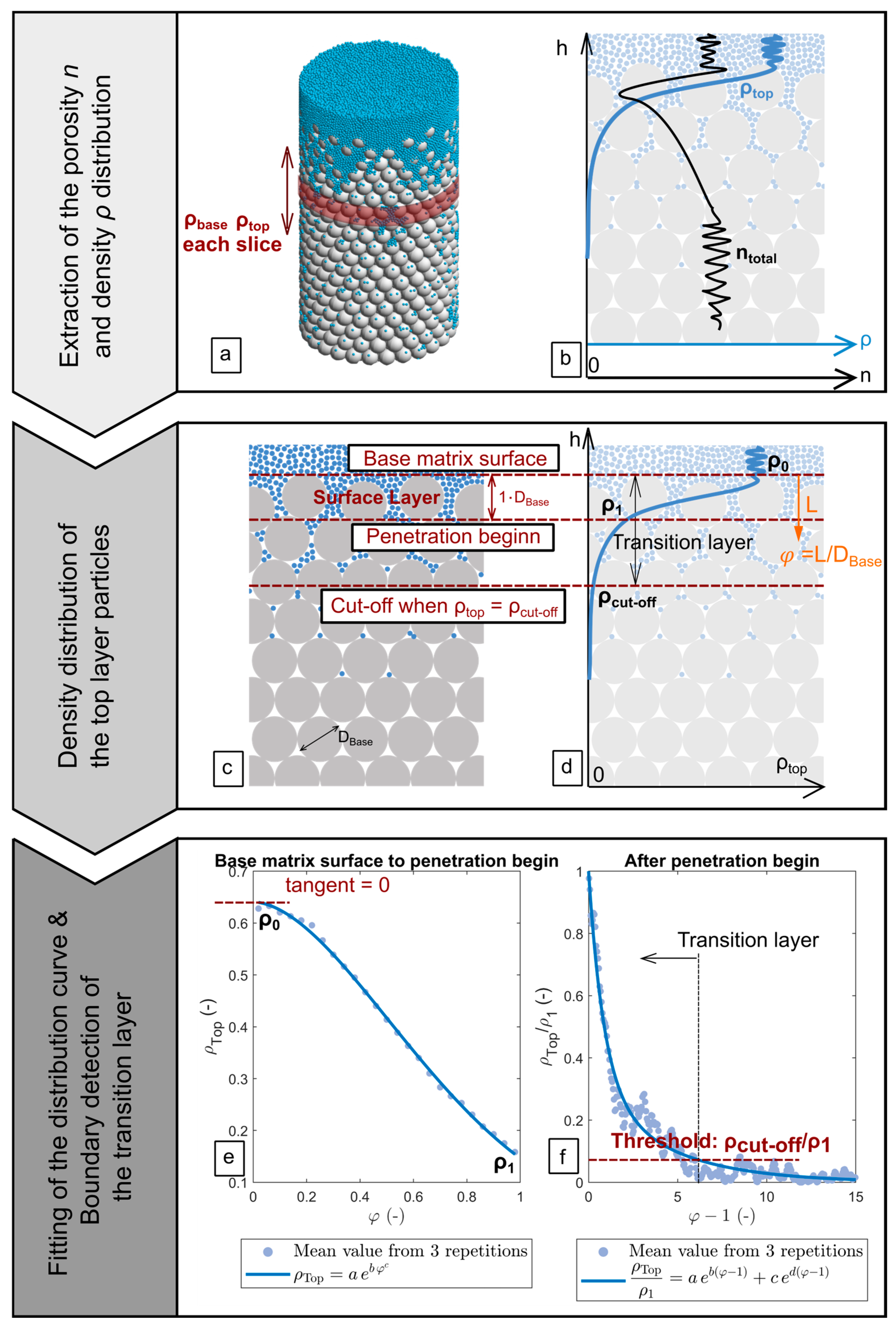
Porosity and Density Distribution Extraction: Consistent with Part I, the porosity and density distributions of stratified samples were extracted from the DEM simulation data by slicing the cylindrical sample along its vertical axis into a series of thin layers (Figure 4a), each with a thickness of min(DBase,DTop)/50. Within each slice, the volume fractions of base-layer and top-layer particles were calculated separately, yielding their respective local densities ρBase and ρTop. The total solid density ρs was obtained as the sum of these two values, and the local porosity was then computed as ntotal = 1 − ρs. This yielded the full vertical porosity profile of the stratified packing (Figure 4b, black line). Additionally, the vertical profile of ρTop was extracted to analyze the extent of infiltration of fine top-layer particles (Figure 4b, blue line).
Figure 4.
(a) Slicing of a sample and calculation of the volumes of top-layer particles, base-layer particles, and all particles within each slice. (b) Calculation of the total porosity distribution of the sample and the vertical distribution of top-layer particle density. (c,d) Schematic illustration of the transition layer boundary determined based on the distribution of top-layer particle density. (e) Exponential fitting of the top-layer particle density distribution between the base matrix surface and the penetration begin line. (f) Exponential fitting of the top-layer particle density distribution below the penetration begin line.
Identification of the Transition Layer: The density profile ρTop typically decreases with depth. This trend forms the basis for defining the transition layer. A density threshold ρcut-off was introduced to define the lower boundary of the transition layer: when the local ρTop falls below this threshold, the influence of infiltrating fine particles on total porosity becomes negligible. The upper boundary of the transition layer is defined by the top surface of the base sediment matrix (Figure 4c,d).
A “penetration begin line” was introduced at a depth of 1 × DBase below the base surface. As established in Part I, this region—referred to as the surface layer—is typically loosely packed, allowing even relatively large particles to accumulate. Below this layer, only smaller particles can penetrate further. Consequently, the ρTop profile was split into two segments for curve fitting, which improves robustness against local noise in data: one above and one below the penetration begin line. This segmentation captures the difference in decay behavior of ρTop—rapid at the surface, slower at greater depth—and allows for the use of different fitting functions (Figure 4e,f). The upper segment follows a compressed exponential function:
Here, ρTop represents the density of top-layer particles at a given depth, and φ denotes the dimensionless penetration depth (Figure 4d).
The lower segment follows a second-order exponential function:
Here, ρ1 denotes the density of top-layer particles at the penetration begin line (Figure 4d).
To remain consistent with Part I, a 2% threshold was used for ρcut-off in this study to determine both the transition layer thickness and the average porosity within the transition layer. The minimum porosity was directly extracted from the ntotal distribution profile.
2.2. Results of Numerical Simulations
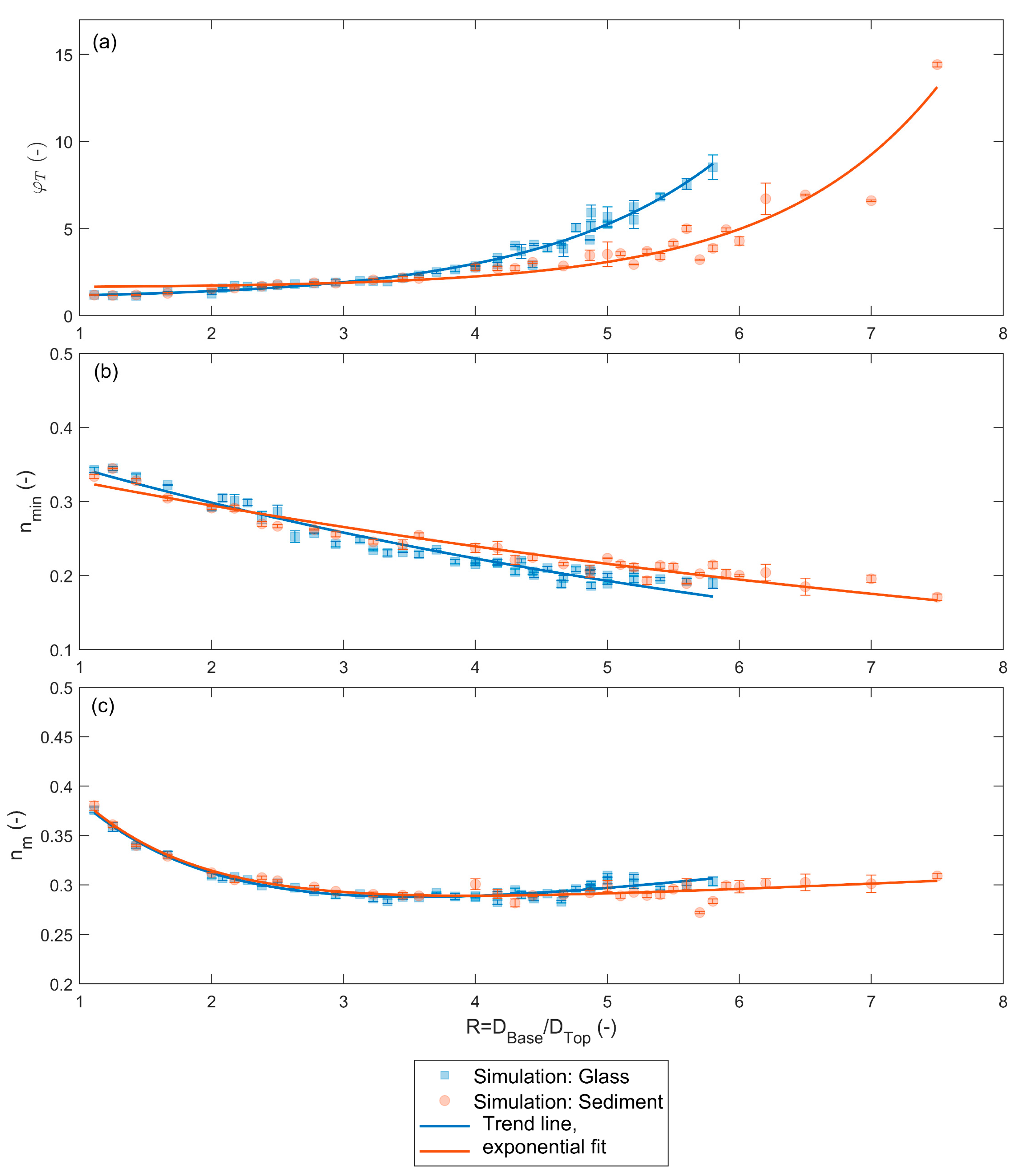
The numerical simulation results using high inter-particle friction coefficients to represent natural sediments in this study are compared with the glass bead simulation results from Part I in Figure 5.
Figure 5.
(a) Relationship between dimensionless transition layer length φT and R; (b) relationship between minimum porosity within the transition layer nmin and R, and (c) relationship between average porosity of the transition layer nm and R for stratified samples numerically generated using glass beads (Data from Part I) and natural sediment.
The effects of particle material (natural sediment or glass beads) on the transition layer length, as well as the average and minimum porosity of the sediment within the transition layer are analyzed. The transition layer boundaries were uniformly determined using the method introduced in Section 3.1.2 (density threshold = 0.02). Except for the defined density threshold of 0.02, the determination of the transition layer length and the average porosity within the transition layer is free from other subjective influences.
Transition Layer Length: As shown in Figure 5a, the relationship between the normalized transition layer thickness φT and the grain-size ratio R for natural sediments can be described by an exponential function. The average measurement error of φT is 0.13. Compared to glass beads, natural sediment samples exhibit significantly lower φT values when R > 3, highlighting the strong inhibitory effect of higher inter-particle friction. In the simulations, the friction coefficient of natural sediment is approximately 2.66 times that of glass beads, which substantially limits the infiltration depth of fine particles. As a result, the critical grain-size ratio R’ for unlimited penetration increases to around 8, consistent with the value of 9.01 reported by []. Notably, simulations at R = 8 show variability—some trials indicate unlimited penetration, while others yield finite depths—suggesting stochastic behavior near the threshold. Therefore, a more stable range of R = 0 to 7.5 was used for curve fitting. Within this range, the relationship between φT and R for natural sediments is well captured by the following empirical equation:
Sediment (1 ≤ R ≤ 7.5):
The influence of inter-particle friction on the percolation of top-layer particles will be discussed in Section 4.1.
Minimum Porosity in the Transition Layer: As shown in Figure 5b, the average measurement error of the minimum porosity nmin for natural sediment is 0.004. For both natural sediment and glass beads, nmin within the transition layer decreases with increasing grain-size ratio R. At R = 1, the minimum porosity is approximately 0.35, which aligns closely with the theoretical porosity of a uniform packing (~0.36). As R approaches the critical grain-size ratio R′, nmin stabilizes around 0.19.
The lower limit of minimum porosity appears to be largely independent of material type. However, across the entire range of R, natural sediment consistently exhibits slightly higher nmin values than glass beads. This difference is likely due to the looser packing arrangement of fine natural sediment particles as they infiltrate the base layer, possibly influenced by higher surface friction. The relationship between nmin and R for natural sediment is captured by the following empirical formula:
Sediment (1 ≤ R ≤ 7.5):
Average Porosity in the Transition Layer: As shown in Figure 5c, the average measurement error of the transition layer average porosity nm is 0.003 for both materials. The results indicate that, within the range R = 1 to 4.5, the average porosity in the transition layer is nearly identical for natural sediment and glass bead samples. In both cases, nm reaches its minimum at approximately R = 3.5, followed by a gradual stabilization around 0.3.
The relationship between nm and R for natural sediment is described by the following empirical equation:
Sediment (1 ≤ R ≤ 7.5):
3. An Empirical Porosity Predictor for Layered Sphere Packings
Based on the dataset generated through numerical simulations, this study further aimed to develop empirical formulas capable of predicting the porosity of stratified sediment structures. It is important to emphasize that, given the focus of this research on the effects of stratification in natural sediments, the derivation of the empirical models presented in this section relies exclusively on simulation data in which the material properties—such as friction and restitution coefficients—were representative of natural sediments, rather than idealized glass spheres from part I.
In principle, the empirical Formulas (5) and (7) presented in Section 3.2 can be applied to determine the unknown values and in the porosity calculation model (Equation (1)), thereby allowing the computation of the average porosity of a stratified system. This straightforward approach was indeed adopted in Part I. However, while effective for porosity estimation, it does not permit the determination of the volume fractions of different particle sizes within a given region, limiting its applicability for analyzing grain-size composition in stratified samples. Consequently, it cannot be integrated with existing models that predict porosity of randomly packed sediments based on particle volume fractions, making it impossible to compare porosity differences between stratified and random samples of the same sediment composition. To address this, the present study attempts to predict the density distribution of the top-layer particles using R as an input parameter. Meanwhile, the density distribution of the base-layer sediment is determined by averaging over multiple samples. By combining these density distributions within a defined region, it becomes feasible to calculate not only the average porosity but also the volume fractions of particles of varying sizes. This methodology is detailed in Section 4.1.
3.1. Methodology
3.1.1. Density Distribution Prediction for Top and Base Layer Particles Based on R
Prediction of Top-Layer Particle Density Distribution: As introduced in Section 3.1.2, the density distribution of top-layer particles between the base matrix surface and the penetration begin line follows a compressed exponential distribution, while below the penetration begin line, it follows a second-order exponential distribution. By analyzing the density of top-layer particles at the penetration begin line ρ1 across different particle size ratios R, it was found that the relationship between ρ1 and R can be well approximated by a second-order polynomial function (Figure A1 in Appendix B, the distribution of ρ1 with respect to R will be further discussed in Section 4.2):
Therefore, for a given R, ρ1 can be determined first. The density of top-layer particles at the base matrix surface ρ0, i.e., the beginning of the transition layer, can be considered a known value (ρ0 = 1 − n0, n0 = 0.36–0.4). For the region from the base matrix surface to the penetration begin line, this implies that the compressed exponential distribution function has known values at φ = 0 and φ = 1. Incorporating these boundary conditions, Equation (2) can be rewritten as:
C is the only remaining unknown parameter.
For the region below the penetration begin line, the density distribution of the top-layer particles is given by Equation (4), where a, b, c, and d are unknown parameters. Among them, a + c must always equal 1 to ensure that ρTop approaches zero as φ approaches infinity. Thus, Equation (4) can be rewritten as:
a, b and d are the remaining unknown parameters.
By varying the value of R and fitting the top-layer particle density distributions derived from numerical simulations using Equations (9) and (10), the values of a, b, d and C for each R can be obtained. Since R is the only variable differing between samples, an attempt is made to establish the relationships between a, b, d, C and R:
To maintain consistency with the mathematical expression in Equation (8), polynomial functions were also chosen for f2 through f5. The fitting results for each parameter are presented in Appendix B. The accuracy of the predicted top-layer particle density distribution based on Equations (8)−(11) will be analyzed in detail in Section 3.2.1.
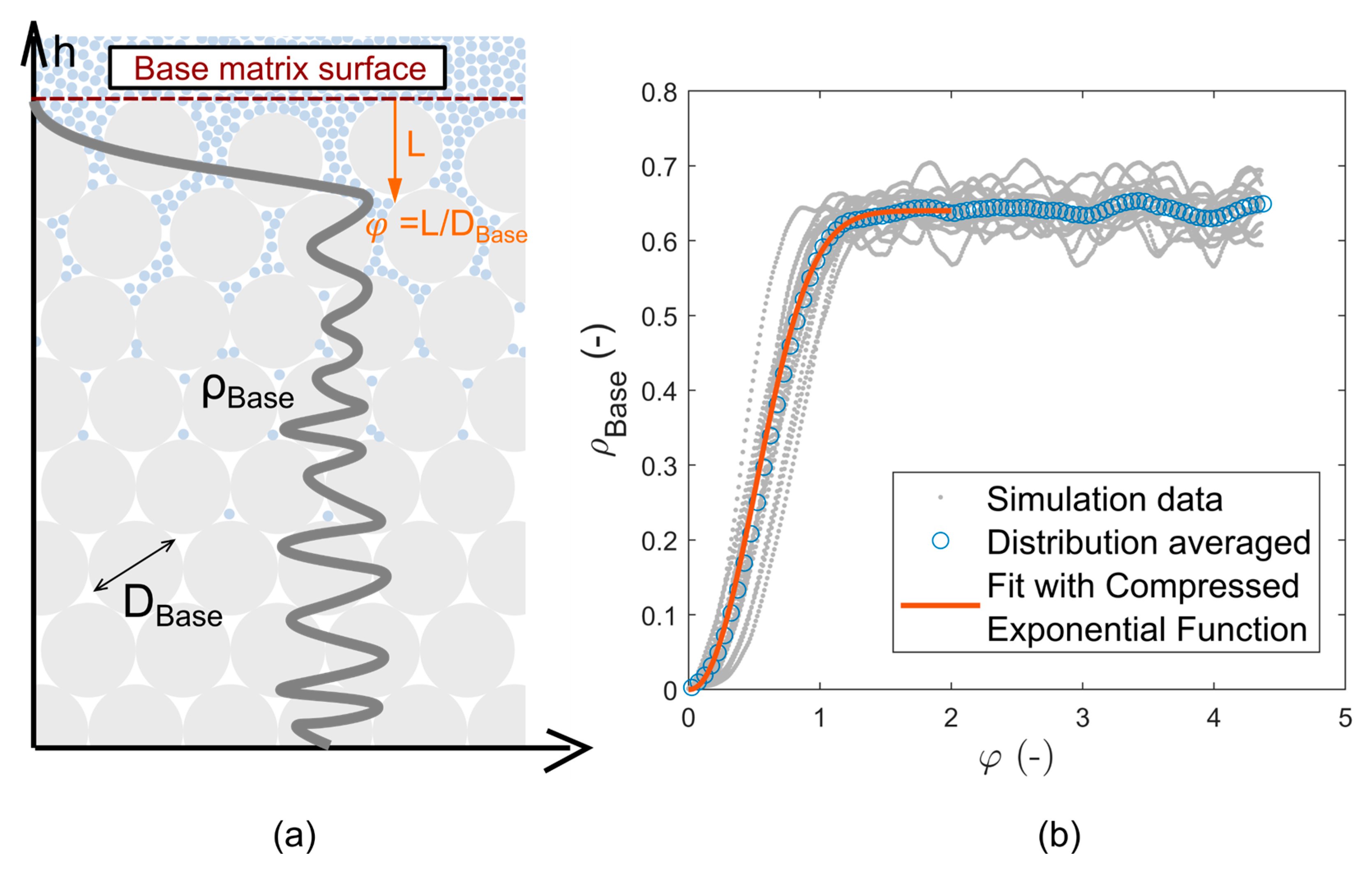
Prediction of Base-Layer Particle Density: Unlike the top-layer particle density distribution introduced in the previous section, the base-layer density distribution ρBase is independent of the particle size ratio R. By analyzing the average base-layer density distribution from over 50 numerically simulated samples (Figure 6), a compressed exponential function was used to describe the relationship between ρBase and the dimensionless depth φ (RMSE = 0.005, R2 = 0.985):
Figure 6.
(a) Distribution of base-layer particle density. (b) Statistical averaging of base-layer particle distributions from multiple samples and exponential fitting of the averaged distribution.
Based on this, within a transition layer of length φT, the average porosity nm, the minimum porosity nmin, and the volume fraction ratio of top-layer to base-layer particles XTop/XBase can be calculated using the following formulas:
3.1.2. Coupling with Yu & Standish—Predictor
To investigate the porosity differences between layered and random samples composed of the same sediments, this study couples the density-distribution-based porosity prediction model introduced in the previous section with the Yu & Standish model [,]. This section considers two limiting cases of layered sediment structures:
No homogeneous sediment layers: This case corresponds to the homogeneous strata 1, 2, and 3 in Figure 1 having zero thickness. It can be regarded as a simplified model of natural sediment deposits where grain size gradually decreases upward without distinct layering. Following previous studies [,] that used sieve analysis to determine sediment composition, this study divides particle sizes from 0.063 mm to 125 mm into 22 groups based on the 0.5 phi sieve set. Sediments within each group are considered uniform in size, with the representative diameter defined as Di = (Dupper × Dlower)0.5, where Dupper and Dlower are the upper and lower diameter bounds of the group (Figure 7a).
Figure 7.
(a) Division of particle sizes within the 0.063–125 mm range into 22 groups. (b) Random selection of N groups as the particle size composition of a stratified sample, in which the homogeneous layer thickness is zero and the sample consists entirely of multiple transition layers. (c) Calculation of the length of each transition layer, the volume fraction of the top-layer and base-layer particles within each transition layer, and the average porosity of the transition layer. (d) Since the base-layer particle size of the (k − 1)-th layer is the same as the top-layer particle size of the k-th layer, the total volume of particles with this size in the entire sample is obtained by summing its volumes in both layers.
Using a MATLAB R2024b program, N groups are selected from these 22 representative diameters, where N ranges between 2 and 22. The selected diameters decrease sequentially from bottom to top to generate layered samples (Figure 7b, with the number of transition layers n = N − 1). This process produces 1000 different grain size combinations. During this, it is ensured that the ratio of diameters between adjacent base- and top-layer sediments does not exceed the critical value R′, thereby preventing infinite penetration.
In the k-th transition layer, the grain diameter of the top-layer sediment is denoted as DTop,k, and that of the base-layer sediment as DBase,k (Figure 7c). The average porosity nm,k within this transition layer can be calculated using Equation (13). Considering the absence of homogeneous sediment layers, the entire sample consists solely of transition layers, so the overall porosity of the sample is given by
where φT,k is the dimensionless thickness of the k-th transition layer. The volume fractions X of the top-layer sediment and base-layer sediment within this transition layer, relative to the entire sample, are given by:
and denote the density distribution curves of the top-layer and base-layer particles, respectively, within the k-th transition layer as functions of φ.
It is worth noting that the grain size of the base-layer sediment in the (k − 1)-th transition layer is identical to that of the top-layer sediment in the k-th transition layer (Figure 7d). Therefore, the volume ratios calculated separately for these two layers need to be summed:
Based on this, the porosity of the stratified sample nstratified with no homogeneous sediment layers and upward-decreasing grain size can be calculated using Equation (16). The volume fraction XD of each grain size within the sample can be determined from Equation (19). These volume fractions are then used as input to the Yu & Standish model to calculate the porosity of the corresponding well-mixed sediment sample nwell-mixed. The two results are compared by computing the ratio k = nstratified/nwell-mixed.
Infinite Homogeneous Sediment Layers: Given that the length of a transition layer φT is a fixed value for a specific grain size ratio, it does not increase with the continued accumulation of the overlying sediment. Therefore, when the thickness of the homogeneous sediment layers becomes much greater than that of the transition layers, the average porosity of the stratified deposit asymptotically approaches n0 (Equation (1)).
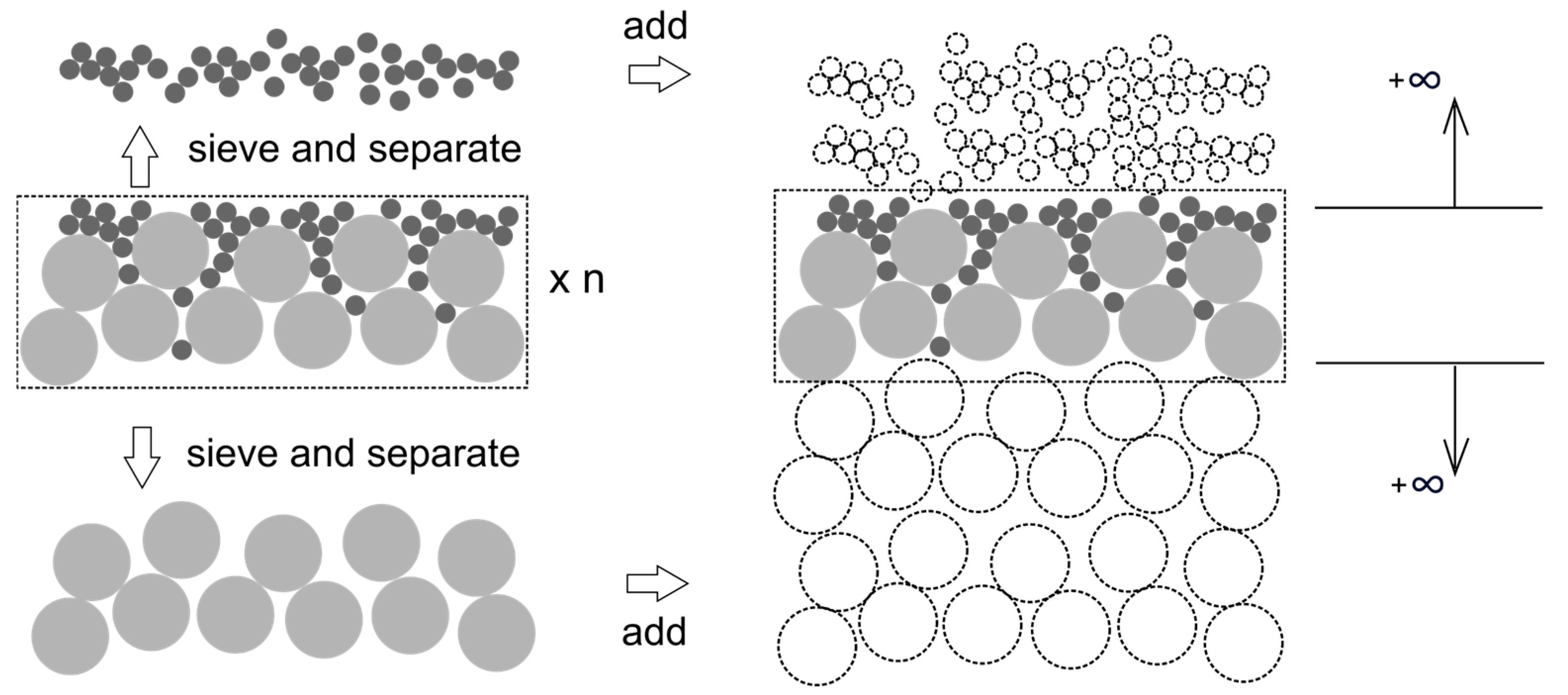
Based on the 1000 grain-size-decreasing sediment samples without homogeneous layers generated in the previous section, this study investigates the limiting case where the thickness of each homogeneous layer is gradually increased while maintaining constant volume fractions for each grain size. As the thickness approaches infinity, nstratified approaches n0. This scenario is conceptually feasible: as illustrated in Figure 8, imagine duplicating a transition layer n times, separating the upper and lower particles by sieving. These sorted particles are then added to the respective upper and lower homogeneous layers to continuously increase their thickness. Throughout this process, the volume fractions of the various grain sizes remain unchanged.
Figure 8.
Schematic diagram illustrating the increase in top- and base-layer sediment thickness while maintaining a constant volume ratio between different particle sizes.
Since the grain size composition remains constant, the porosity of a well-mixed sediment sample calculated via the Yu & Standish model, nwell-mixed, remains constant. The porosity ratio under this limiting condition, k = nstratified/nwell-mixed = n0/nwell-mixed, is then computed.
3.2. Results of Empirical Predictor
3.2.1. Performance Check
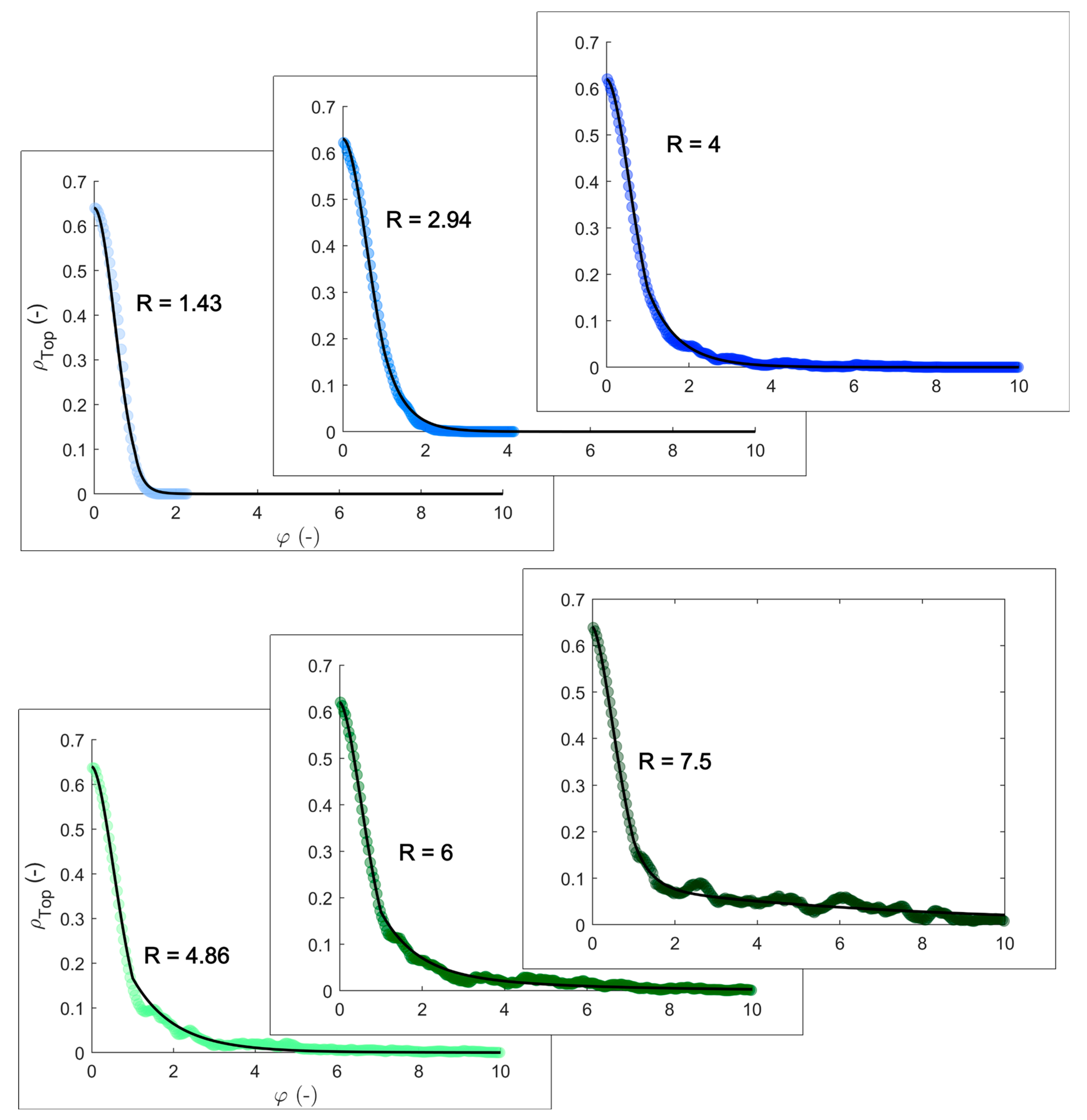
Using the empirical models (8)–(11), the density distribution curves of infiltrating top-layer particles can be predicted. As shown in Figure 9, six measured infiltrating particle density curves for different R values from the numerical simulations are presented as examples. For comparison, the predicted distribution curves from the empirical models are shown as black solid lines. It can be observed that the predicted curves closely match the measured ones.
Figure 9.
A comparison between the measured and predicted distributions of top-layer particle density is presented, where the predicted distributions are shown as black solid lines, and the measured distributions are represented by circular markers.
By comparing all measured and predicted curves and calculating the RMSE and correlation coefficient R2 between them, the prediction error for the ρTop distribution ranges from 0.004 to 0.08. The correlation coefficients between predicted and measured curves lie between 0.96 and 0.99. Therefore, empirical models (8)–(11) are considered capable of accurately predicting the density distribution of infiltrating top-layer particles within the base sediment layer.
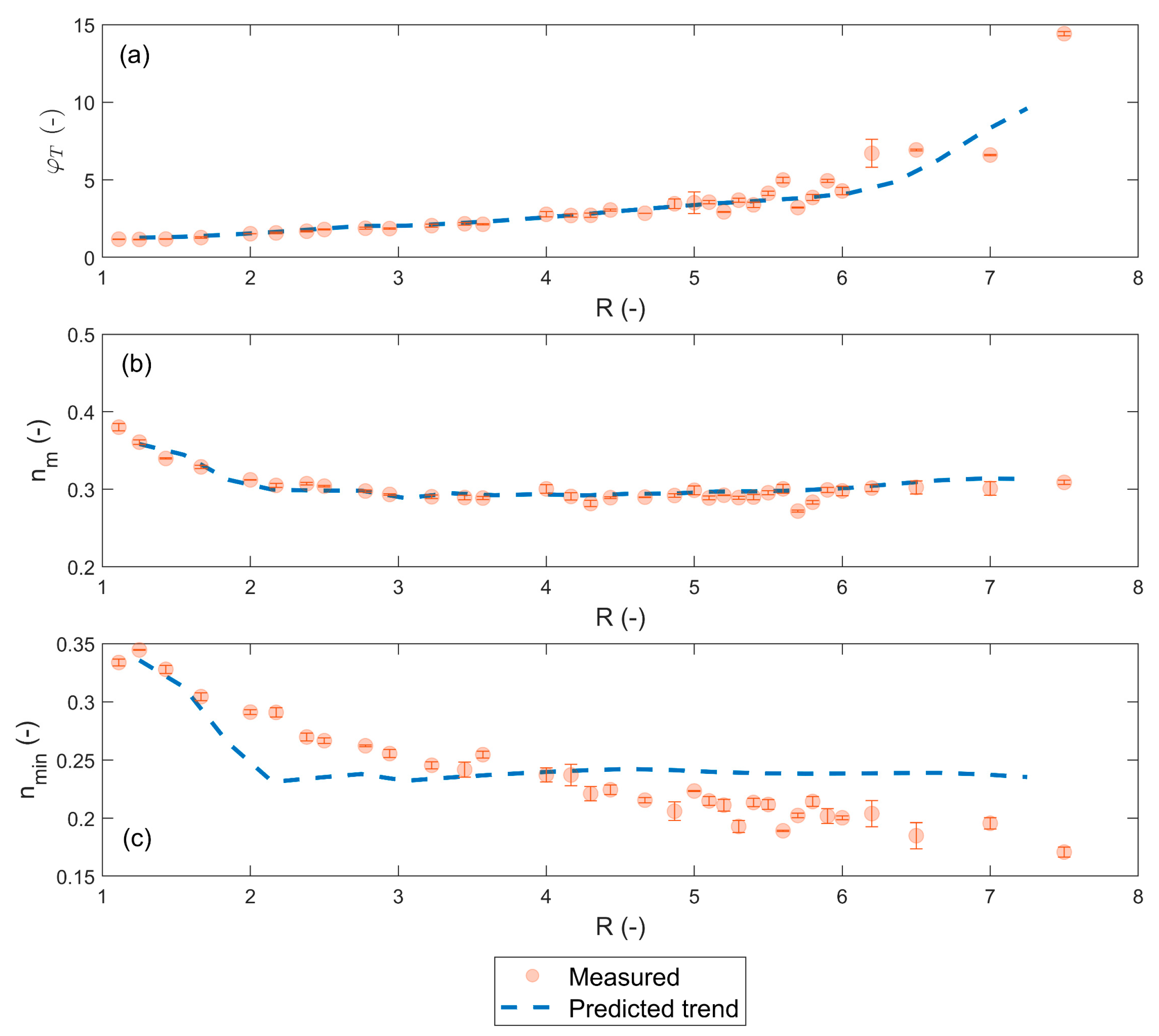
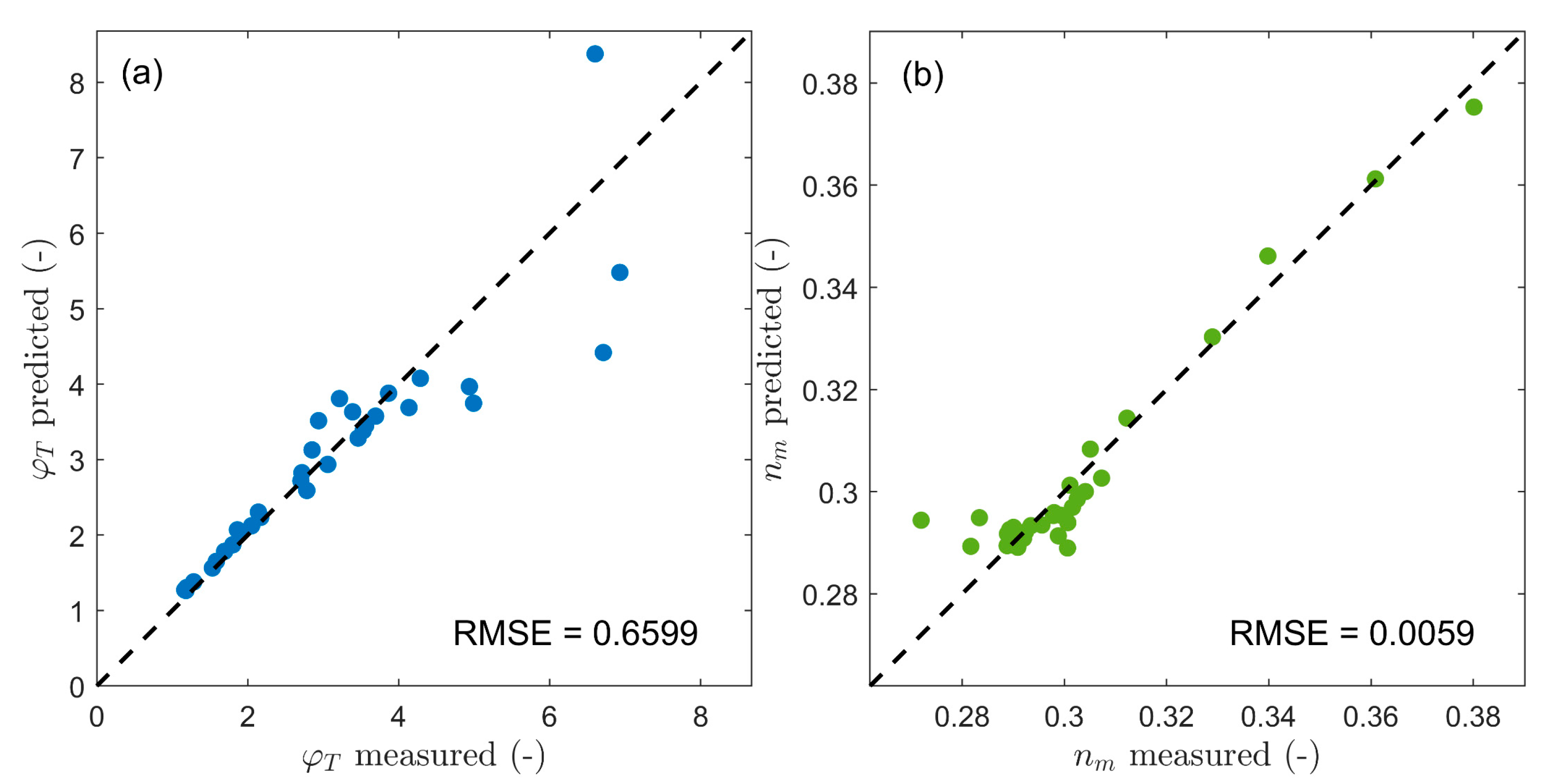
Based on the empirical models (8)–(12), this study further calculated the predicted transition layer length φT for each R value. Simultaneously, predictions for nmin and nm were obtained using Equations (13) and (14). In Figure 10 and Figure 11, the measured values of these three parameters are compared with their corresponding predictions from the empirical formulas.
Figure 10.
(a) Comparison between measured values and predictions from the empirical model for dimensionless transition layer length φT; (b) comparison between measured values and predictions for average porosity of the transition layer nm, and (c) comparison between measured values and predictions for minimum porosity nmin within the transition layer as functions of R.
Figure 11.
(a) Comparison of measured and empirical model predicted values of dimensionless transition layer length φT. (b) Comparison of measured and empirical model predicted values of average porosity within the transition layer nm.
It is worth noting that the use of the empirical models requires specifying the density of top-layer particles ρ0 at the start of the transition layer. Since all sediment samples generated in this study’s numerical simulations are dense, a uniform value of ρ0 = 0.64 (ρ0 = 1 − n0, n0 = 0.36 for dense packing) was adopted for further calculations.
As shown in Figure 10a, the empirical model can accurately predict the transition layer length φT within the range of R = 1 to 6 (corresponding to φT values less than 5). When R exceeds 6, due to the large variability observed in the measured data itself, the absolute error between the predicted and measured values increases (corresponding to points where φT is greater than 5 in Figure 11a). However, the upward trend in the measured data is still well captured by the predictions.
Similarly, the measured and predicted average porosity values nm nearly coincide (Figure 10b), with an RMSE of only 0.006. The empirical formula accurately predicts the average porosity for each R value.
In contrast to the accurate predictions for φT and nm, the empirical model shows a significant deviation when predicting the minimum porosity nmin, which represents a major limitation of the empirical models introduced in Section 4. The causes of this deviation will be further discussed in Section 4.3. According to Equation (1) for calculating the overall porosity of the layered sample, the total porosity is influenced only by the average porosity of each transition layer. Therefore, this limitation in accurately predicting nmin does not affect the model’s applicability for calculating the total porosity of layered samples.
3.2.2. nstratified Versus nwell-mixed
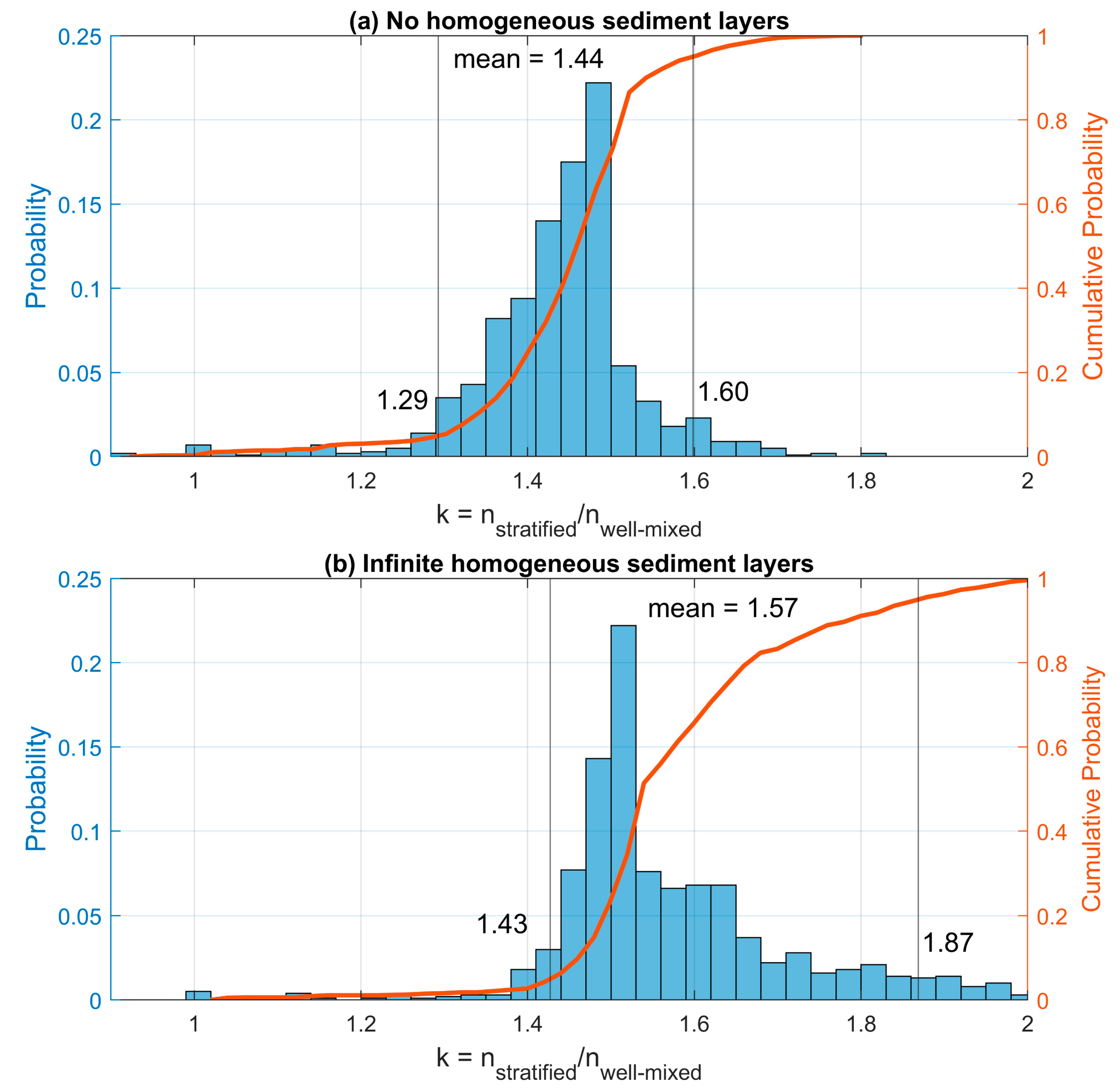
The porosity differences between the layered samples and the well-mixed samples under no homogeneous sediment layers and infinite homogeneous layers are presented in Figure 12a,b.
Figure 12.
(a) Probability distribution of the porosity ratio k between stratified samples with no homogeneous layers and well-mixed samples with the same sediment composition; (b) Probability distribution of k between stratified samples with infinite homogeneous layers and well-mixed samples.
Cases without homogeneous sediment layers: The statistical analysis of the parameter k (defined as k = nstratified/nwell-mixed) was conducted. The probability distribution of k shows a clear left skew, and the Kolmogorov–Smirnov test [] indicates a non-normal distribution (p-value = 0 ≤ 0.05). Therefore, the cumulative probability curve of the k distribution was plotted. The k values corresponding to the 5% and 95% cumulative probabilities were read as 1.29 and 1.60, respectively, meaning 5% of the samples have k values below 1.29 and 5% above 1.60, thus excluding 10% of extreme values. It can be seen that for 90% of the layered samples without homogeneous layers, the porosity is 1.29 to 1.6 times that of the well-mixed samples with the same sediment composition. After excluding extremes, the average k value is 1.44. This confirms the hypothesis that sediment layering indeed leads to increased porosity due to insufficient mixing of particles of different sizes.
It is worth noting that increasing the sample size from 1000 to 2000 did not show a significant change in the probability distribution of k, indicating that the sample size is sufficiently large to ensure statistical reliability and robustness of the conclusions.
Cases with infinite homogeneous sediment layers: The probability distribution of k is clearly right-skewed, with more values above the mean. The k values at 5% and 95% cumulative probabilities are 1.43 and 1.87, respectively. After excluding extremes, the average k value is 1.57. This extreme sediment layering condition further increases the total sediment porosity.
Under realistic conditions, layered sediments are considered to fall between these two extremes. Based on the theoretical calculations of this study, compared with fully mixed sediments, layering phenomena in sediments may lead to a porosity increase ranging from 144% to 157%.
4. Discussion
4.1. Discussion on the Influence of Inter-Particle Friction on the Transition Layer Length
Before discussing the influence of the friction coefficient on the transition layer length, it is necessary to briefly explain the infiltration process of top layer small spheres into the base layer sediment. According to elementary geometry, smaller particles can percolate through the pores between larger particles. When percolation is possible, the particle size ratio between the large and small spheres is referred to as the critical size ratio Rc. In the case of cubic packing of spheres (porosity 0.476), Rc equals 2.42; for tetrahedral packing (porosity 0.260), Rc equals 6.45. Since the porosity of random uniform sphere packings lies between 0.36 and 0.4, the corresponding Rc should be between 2.42 and 6.45. Simulation results (Figure 5a) show that when R is greater than 3, the transition layer length significantly increases, and infiltration of top layer particles becomes pronounced. It is thus inferred that the Rc of the random sample is approximately 3.
It is important to emphasize that R > Rc only indicates that small particles can pass through the pores between large particles. However, because the channels formed by pores between large particles are winding and tortuous, particles moving within them may encounter “dead-end-pores” and stop moving forward. When many small particles need to pass through the same channel, a “bridging effect” may occur due to particle shape and frictional interactions, clogging the channel and limiting further infiltration.
The bridging or clogging effect—where smaller particles accumulate at the entrances of larger pores and inhibit further infiltration—is a widely recognized phenomenon across granular flow and sediment transport studies [,,,,]. Experimental and theoretical work has shown that when the pore throat size is only marginally larger than the infiltrating particle diameter, stable particle arches can form, obstructing deeper penetration [,]. The larger the small particles, the higher the probability of bridging. Conversely, smaller particles reduce the likelihood of bridging and increase infiltration depth.
When more small spheres accumulate at the blockage, the additional gravitational force may exceed the frictional force supporting the bridge, breaking it and allowing particles to continue infiltrating. When the inter-particle friction coefficient increases, the probability of blockage rises while the likelihood of breaking the bridge decreases, leading to a significant reduction in infiltration depth. However, correspondingly, due to the difficulty of infiltration under high friction, unlimited infiltration only occurs when the small particles become sufficiently small. Compared to glass spheres, natural sediment has a friction coefficient approximately 2.66 times higher. This explains why natural sediment exhibits significantly shallower infiltration depths than glass spheres, yet possesses a larger critical R′ value.
4.2. Discussion on the Empirical Porosity Predictor for Stratified Packings
Structure of the Empirical Model: When predicting the infiltration density curve of the top layer sediment, the empirical model divides the distribution curve into two segments: from the base matrix surface to the penetration begin line 0 ≤ φ ≤ 1, and below the penetration begin line φ ≥ 1. The density of the top layer sediment at φ = 0, ρ0, can be determined from the theoretical porosity n0 of a uniform random packing, which ranges from 0.36 to 0.4 (ρ0 = 1 − n0). It was later found that the density of the top layer sediment at φ = 1, denoted as ρ1, can also be expressed by an empirical formula. These two values, ρ0 and ρ1, therefore serve as known control points for the infiltration density profile of the top layer sediment.
In fact, it is theoretically possible to use only ρ0 as a known quantity to predict the density distribution in the segment 0 ≤ φ ≤ 1 and solve for ρ1, then use ρ1 to further predict the distribution for φ ≥ 1. However, lacking ρ1 as a known control value at the connection of the two segments may cause errors in predicting the density in the segment 0 ≤ φ ≤ 1 to accumulate into the segment φ ≥ 1, thereby reducing the overall accuracy of the model prediction.
It is worth mentioning that although the initial reason for dividing the distribution curve into segments was the inability to fit a single function over the entire range φ ≥ 0, a possible theoretical explanation for this segmentation can be provided. In Figure 5a, the φT-R curve shows that even when R is less than Rc (approximately 3 for random samples, see previous section), the measured transition layer length is not zero but roughly stable at φT = 1. This indicates that top layer particles, which theoretically should not be able to pass between the base layer particles, can still move across the surface of the base matrix and accumulate within a range of approximately one DBase below it. This phenomenon mainly occurs because near the base matrix surface, the porosity and inter-particle voids increase significantly. This sediment layer, characterized by noticeably looser packing, is commonly defined as the surface layer. Wooster et al. [] pointed out that the thickness of this layer is typically about twice DBase.
However, through studying the average base sediment density distributions of over 50 numerically simulated samples (Figure 6), it was found that the base sediment density distribution follows . Calculations show that: ρBase(φ = 1)/ρBase(φ = ∞) = 0.909, ρBase(φ = 1.5)/ρBase(φ = ∞) = 0.997. This means that at a depth of one DBase below the base matrix surface, the particle packing density has already reached about 90% of its maximum value, and by 1.5 × DBase, the particles are arranged nearly as densely as possible. Because this loosely packed surface layer is relatively thin, when the particle sizes of the top and base layers are similar, top layer particles can only accumulate within approximately one DBase below the base matrix surface and are unable to infiltrate deeper.
Based on this, the study proposes the following summary: For the range 0 ≤ φ ≤ 1, the transition layer forms mainly through the filling of pores in the loosely packed surface layer of the base matrix by top layer particles—referred to as the filling mechanism. The segment can already build when 1 ≤ R ≤ Rc. For φ ≥ 1, small particles infiltrate through the pores between larger base particles and penetrate to varying depths—referred to as the infiltration mechanism. The existence of this segment requires that the size ratio R exceeds the critical value Rc.
Density ρ1 at Penetration Begin Line: As mentioned in the previous section, the density ρ1 at the penetration begin line can be determined empirically as a function of R, with its distribution detailed in Appendix B. The ρ1-R relationship shows that when R > 3, ρ1 stabilizes at approximately 0.18 (Figure A1).
In fact, based on the previously described filling mechanism, a theoretical estimation of ρ1 can be attempted. At the penetration begin line (i.e., one DBase below the base matrix surface), the packing density of the base layer particles is nearly equivalent to that in the deeper part of the sample. Assuming a base layer porosity nBase = 0.36, the available pore volume for infiltration particles at this location is nBase × V, where V is the control volume encompassing both solid particles and pores. Given that the top layer sediment settles without any additional vibration, the top-layer particles in the pores of base-layer particles is presumed to form a loose to very loose packing [], with a porosity n ranging from 0.40 to 0.44. Thus, the volume of infiltrating particles within the control volume is approximately nBase × V(1 − n), which yields a theoretical density value for ρ1 between 0.202 and 0.216 (calculated by nBase × (1 − n)).
The experimentally observed ρ1 is slightly lower. This discrepancy is likely due to the high inter-particle friction coefficient used in the simulation and the absence of vibration, both of which hinder the small particles from fully occupying the pore space between larger particles. Furthermore, each large particle acts as a rigid boundary to the surrounding small particles, creating a wall effect that results in looser local packing and thus increases n. It is therefore inferred that the actual n may be closer to 0.49–0.50, in which cases the theoretical density matches the observed ρ1 values more closely.
Model Limitations: As discussed in Section 3.2.1 on the predictive accuracy of the empirical model, the model exhibits a noticeable deviation when estimating the minimum porosity within the transition layer (Figure 10c). This minimum value is calculated using the equation: . Here, the distribution of ρBase is derived by averaging the base layer density distributions from over 50 numerical simulation samples, and fitting the result to an empirical function. This distribution represents a statistical average, which inevitably differs from the ρBase distribution in any individual sample. In other words, for a given size ratio R, a slight mismatch may exist between the predicted distributions of ρTop and ρBase compared to the actual sample.
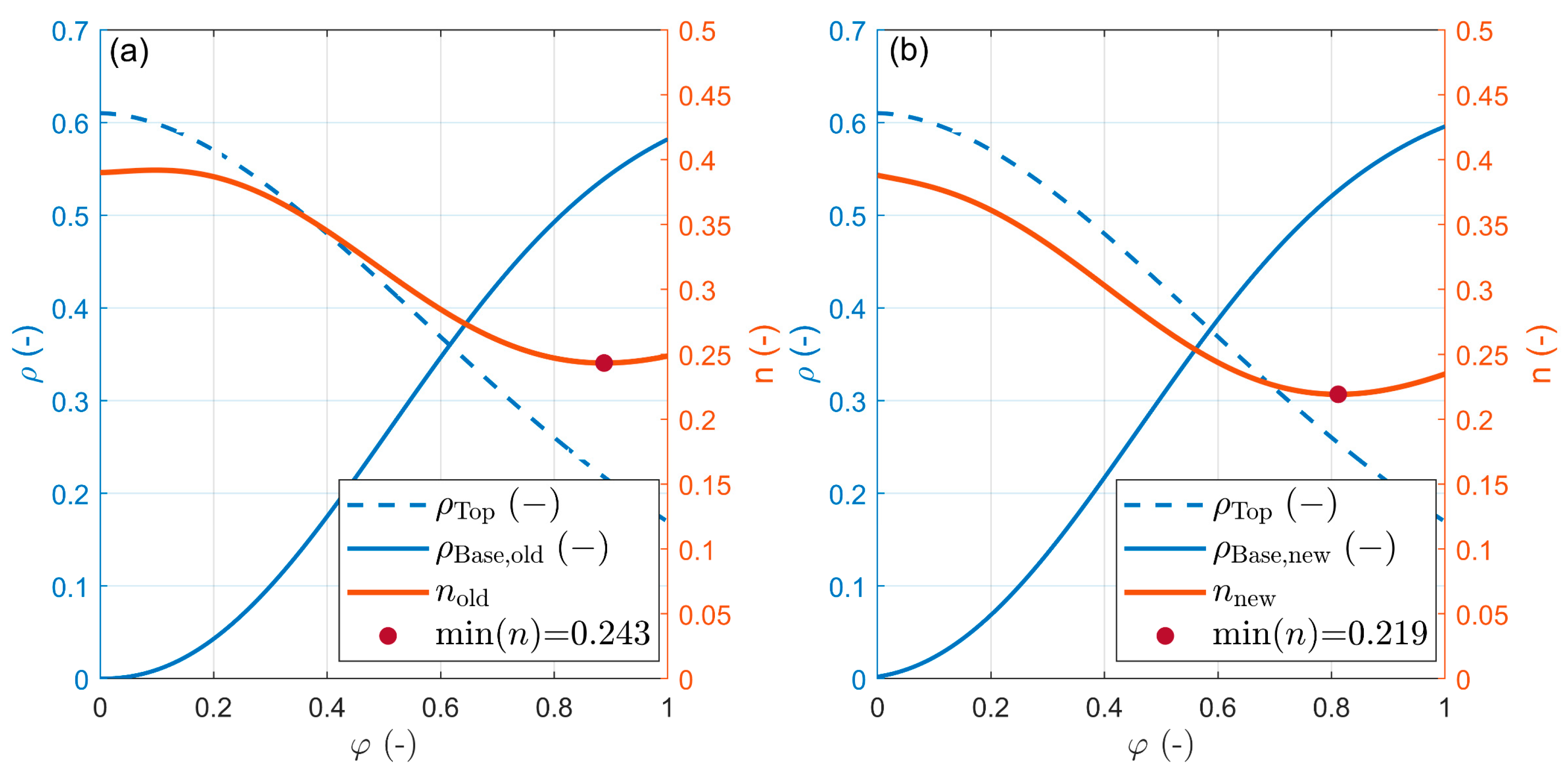
Figure 13a illustrates the process of computing nmin for R = 5 using the empirical model. In comparison, Figure 13b shows a case where the ρBase,new distribution is shifted 0.05 units to the left relative to the original ρBase,old in Figure 13a. This small misalignment directly reduces the predicted minimum porosity from 0.243 to 0.219, bringing it much closer to the measured value. This demonstrates that the prediction of nmin is highly sensitive to any offset between the ρTop and ρBase distributions.
Figure 13.
Calculation of the minimum porosity within the transition layer based on the density distributions of top- and base-layer particles, where in (b) the base-layer particle density distribution is shifted 0.05 units to the left relative to the base-layer density distribution in (a).
However, as shown in Figure 10b, such minor misalignments do not significantly affect the accuracy of the predicted average porosity within the transition layer. This is because a slight shift in ρBase does not substantially alter the volume fraction of base layer particles over an extended region. To support this, the volume fractions were calculated by integrating both ρBase,old and ρBase,new over the range [0, φ] where φ = 1, 2, 3, …, 10. The results, summarized in Table 2, show that the prediction error in base layer volume fraction caused by the shift in ρBase diminishes rapidly as the transition layer length increases. Even in the case of φ = 1, where the maximum error is 0.03, the impact on the porosity prediction using the Yu & Standish model [,] for a well-mixed mixture is almost negligible.
Table 2.
Comparison of volume fractions of base-layer particles within the same range, each calculated based on base-layer particle density distributions with a phase difference of 0.05.
4.3. Discussion on the Effect of Stratification on Packing Porosity
This study compares the porosity of stratified sediment with that of homogeneously mixed sediment of the same grain-size composition by coupling the empirical model with the Yu & Standish model [,]. The results reveal that stratification can lead to a 144% to 157% increase in porosity. As hypothesized, low porosity only occurs within the transition layer of stratified samples due to the mixing of particles with different grain sizes. In contrast, the homogeneous layers maintain porosity values between 0.36 and 0.4. Because the different-sized particles are not well mixed, the voids between large particles cannot be effectively filled by smaller ones, resulting in an overall increase in porosity.
It is important to note that the aim of this study was to generate samples with the maximum possible infiltration depth of top-layer particles. To this end, sample generation were conducted under low sediment dropping rate. Additionally, the infiltration process was not influenced by shear stress from water flow. However, previous studies (e.g., [,,,]) have shown that higher sediment dropping rate and flow-induced shear forces tend to reduce sediment infiltration depth. Furthermore, the irregular shapes of natural sediment particles may promote bridging effects during infiltration, which can block the infiltration pathways and shorten the transition layer. As the transition layer becomes thinner, the proportion of homogeneous layers increases, resembling the limiting case of an infinitely homogeneous sediment layer. Therefore, it is inferred that in natural river environments, the porosity increase due to stratification may be closer to the upper bound of 157%.
Taken together, these findings underscore the importance of accounting for particle-scale and process-scale parameters when modeling sedimentary structures and properties. While the empirical model presented here successfully predicts porosity variations under controlled conditions, its application to natural environments requires further refinement. In particular, incorporating the effects of grain shape and hydrodynamic conditions during deposition will be crucial for improving model reliability. Future research should aim to systematically quantify these variables and their interactions, offering a more holistic understanding of sediment infiltration and packing behavior in stratified deposits.
5. Conclusions and Outlook
This second part of the study expands upon Part I by incorporating realistic friction coefficients representative of natural sediments into DEM simulations to assess their impact on stratification-induced porosity patterns. The key findings and conclusions of this study are as follows:
Results confirm that higher inter-particle friction significantly reduces fine-particle infiltration depth and increases the critical grain-size ratio required for unrestricted penetration. Empirical formulas were derived to predict transition layer thickness and porosity metrics.
A density-distribution-based empirical model was developed to compute the volume fractions and porosity of stratified deposits. By coupling this model with the Yu & Standish predictor for well-mixed sediments, the porosity increase due to stratification was quantitatively evaluated. Findings show that stratified structures exhibit porosity increases of up to 57% compared to uniformly mixed packings.
The introduced density-distribution-based empirical model performs reliably in predicting average porosity and transition layer extend, though limitations exist in estimating minimum porosity due to statistical variability in base-layer density distributions.
The insights gained from this study provide a deeper understanding of how stratification and particle-scale interactions affect porosity in natural sediments. These highlight the importance of considering sediment stratification when modeling riverbed porosity and pave the way for improved sediment transport and hydraulic predictions. Future work should aim to incorporate additional factors such as grain shape and hydrodynamic forces to further enhance predictive capabilities.
Author Contributions
Conceptualization, W.X.; methodology, W.X.; software, W.X.; validation, W.X.; formal analysis, W.X.; investigation, W.X.; resources, W.X.; data curation, W.X.; writing—original draft preparation, W.X.; writing—review and editing, C.B.; visualization, W.X.; supervision, C.B. All authors have read and agreed to the published version of the manuscript.
Funding
This study was funded by the German Research Foundation (Deutsche Forschungsgemeinschaft, Grant Number SCHU 1054/6-2).
Institutional Review Board Statement
Not applicable.
Informed Consent Statement
Not applicable.
Data Availability Statement
The original data presented in the study are openly available in Zenodo at (https://zenodo.org/records/15680592).
Acknowledgments
The effort of the crew of the Model construction and the Metrology during the laboratory experiments is appreciated. We deeply thank our students (Mingxuan Bao, Zhen Wei and Yan Chen) for their support during the numerical simulations.
Conflicts of Interest
The authors declare no conflicts of interest.
Abbreviations
The following abbreviations are used in this manuscript:
| DTop and DBase | diameter of the top-layer and base-layer spheres |
| DGrain | diameter of spheres in a measurement container |
| DContainer | diameter of the measurement container |
| n | porosity value measured within a container of finite size |
| n0 | porosity value measured in an infinitely large container |
| nm | the average porosity of the transition layer |
| nmin | the minimum porosity within the transition layer |
| ntotal | porosity value in a slice (1 − ρSolid) |
| nstratified | average porosity of a stratified structure |
| nwell-mixed | porosity of a well-mixed sediment sample |
| ρBase | density of the base-layer particles in a slice |
| ρTop | density of the top-layer particles in a slice |
| ρsolid | density of all particles in a slice (ρBase + ρTop) |
| ρcut-off | density threshold to identify the lower boundary of the transition layer |
| ρ0 | density of top-layer particles at the base matrix surface |
| ρ1 | density of top-layer particles at the penetration begin line |
| R | size ratio between the top-layer and base-layer spheres (DBase/DTop) |
| Rc | critical size ratio between the large and small spheres when percolation of small particles is possible |
| R′ | critical value of R corresponding to the onset of unlimited percolation of top-layer particles |
| LTransition_Layer | length of the transition layer |
| φ | dimensionless penetration depth |
| φT | dimensionless transition layer length (LTransitionLayer/DBase) |
| X | volume fraction of particles with a certain size |
Appendix A
Table A1.
Particle size ratios used in the numerical simulations.
Table A1.
Particle size ratios used in the numerical simulations.
| Simulation with Natural Sediments | |||
|---|---|---|---|
| DBase - Dtop (mm) | R | DBase - Dtop (mm) | R |
| 10-9 | 1.11 | 14-3 | 4.67 |
| 10-8 | 1.25 | 14.6-3 | 4.87 |
| 10-7 | 1.43 | 15-3 | 5.00 |
| 10-6 | 1.67 | 15.3-3 | 5.10 |
| 10-5 | 2.00 | 15.6-3 | 5.20 |
| 10-4.6 | 2.17 | 15.9-3 | 5.30 |
| 10-4.2 | 2.38 | 16.2-3 | 5.40 |
| 10-4 | 2.50 | 16.5-3 | 5.50 |
| 10-3.6 | 2.78 | 16.8-3 | 5.60 |
| 10-3.4 | 2.94 | 17.1-3 | 5.70 |
| 10-3.1 | 3.23 | 17.4-3 | 5.80 |
| 10-2.9 | 3.45 | 17.7-3 | 5.90 |
| 10-2.8 | 3.57 | 18-3/21-3.5 | 6.00 |
| 12-3 | 4.00 | 21.7-3.5 | 6.20 |
| 12.5-3 | 4.17 | 19.5-3/22.75-3.5 | 6.50 |
| 12.9-3 | 4.30 | 21-3/24.5-3.5 | 7.00 |
| 13.3-3 | 4.43 | 26.25-3.5 | 7.50 |
Appendix B
The density ρTop(φ) is defined piecewise as:
Given:
- ρ0 = 1 − n0 (n0 = 0.36–0.4)
- ρ1 = k1R3 + k2R2 + k3R + k4
- a = log(ρ1/ρ0)
- b = k5R + k6
- c = k7R2 + k8R + k9
- d = k10R2 + k11R + k12
- f = 1 − c
- g = k13R2 + k14R + k15
Table A2.
Empirical coefficients.
Table A2.
Empirical coefficients.
| Coefficient | R ≤ 2 | 2 < R < 3 | R ≥ 3 |
|---|---|---|---|
| k1 | 0 | 0 | 0 |
| k2 | 0.1258 | 0.0020 | 0.0020 |
| k3 | −0.2797 | −0.0193 | −0.0193 |
| k4 | 0.2355 | 0.2132 | 0.2132 |
| k5 | −0.0575 | −0.0575 | −0.0575 |
| k6 | 2.0429 | 2.0429 | 2.0429 |
| k7 | 0 | 0 | −0.0420 |
| k8 | −0.5149 | −0.5149 | 0.4277 |
| k9 | 1.4955 | 1.4955 | −0.2786 |
| k10 | 0 | 0 | −0.2931 |
| k11 | 1.4343 | 1.4343 | 3.0952 |
| k12 | −6.5978 | −6.5978 | −9.1680 |
| k13 | −2.5594 | −2.5594 | −0.0827 |
| k14 | 14.7797 | 14.7797 | 1.2033 |
| k15 | −23.3567 | −23.3567 | −4.5205 |
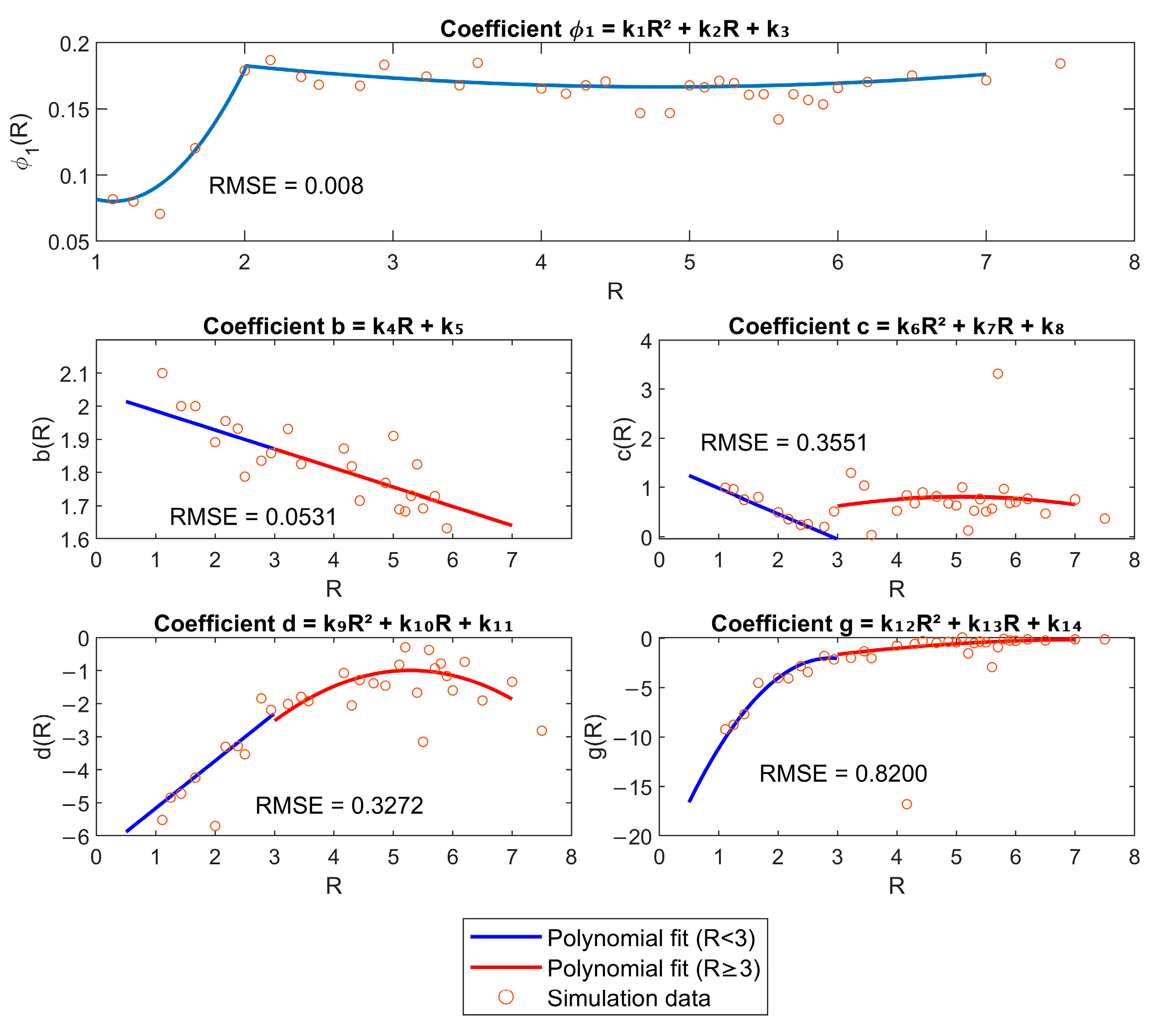
Figure A1.
Determination of different coefficients of the empirical model through fitting.
References
- Chwang, A.T.; Chan, A.T. Interaction Between Porous Media and Wave Motion. Annu. Rev. Fluid Mech. 1998, 30, 53–84. [Google Scholar] [CrossRef]
- Ting, C.-L.; Lin, M.-C.; Cheng, C.-Y. Porosity effects on non-breaking surface waves over permeable submerged breakwaters. Coast. Eng. 2004, 50, 213–224. [Google Scholar] [CrossRef]
- Frings, R.M.; Kleinhans, M.G.; Vollmer, S. Discriminating between pore-filling load and bed-structure load: A new porosity-based method, exemplified for the river Rhine. Sedimentology 2008, 55, 1571–1593. [Google Scholar] [CrossRef]
- Frings, R.M. Sedimentary Characteristics of the Gravel-Sand Transition in the River Rhine. J. Sediment. Res. 2011, 81, 52–63. [Google Scholar] [CrossRef]
- Vollmer, S.; Kleinhans, M.G. Predicting incipient motion, including the effect of turbulent pressure fluctuations in the bed. Water Resour. Res. 2007, 43, W05410. [Google Scholar] [CrossRef]
- El Kadi Abderrezzak, K.; Die Moran, A.; Tassi, P.; Ata, R.; Hervouet, J.-M. Modelling river bank erosion using a 2D depth-averaged numerical model of flow and non-cohesive, non-uniform sediment transport. Adv. Water Resour. 2016, 93, 75–88. [Google Scholar] [CrossRef]
- Miwa, H.; Parker, G. Effects of sand content on initial gravel motion in gravel-bed rivers. Earth Surf. Process. Landf. 2017, 42, 1355–1364. [Google Scholar] [CrossRef]
- Mulatu, C.A.; Crosato, A.; Moges, M.M.; Langendoen, E.J.; McClain, M. Morphodynamic Trends of the Ribb River, Ethiopia, Prior to Dam Construction. Geosciences 2018, 8, 255. [Google Scholar] [CrossRef]
- Frings, R.M.; Hillebrand, G.; Gehres, N.; Banhold, K.; Schriever, S.; Hoffmann, T. From source to mouth: Basin-scale morphodynamics of the Rhine River. Earth-Sci. Rev. 2019, 196, 102830. [Google Scholar] [CrossRef]
- van Bui, H.; Bui, M.D.; Rutschmann, P. Advanced Numerical Modeling of Sediment Transport in Gravel-Bed Rivers. Water 2019, 11, 550. [Google Scholar] [CrossRef]
- Hatch, C.E.; Fisher, A.T.; Ruehl, C.R.; Stemler, G. Spatial and temporal variations in streambed hydraulic conductivity quantified with time-series thermal methods. J. Hydrol. 2010, 389, 276–288. [Google Scholar] [CrossRef]
- Athy, L.F. Density, Porosity, and Compaction of Sedimentary Rocks. Bulletin 1930, 14, 1–24. [Google Scholar] [CrossRef]
- Vollmer, S.; Ramos, F.d.L.S.; Daebel, H.; Kühn, G. Micro scale exchange processes between surface and subsurface water. J. Hydrol. 2002, 269, 3–10. [Google Scholar] [CrossRef]
- Noack, M.; Ortlepp, J.; Wieprecht, S. An Approach to Simulate Interstitial Habitat Conditions During the Incubation Phase of Gravel-Spawning Fish. River Res. Appl. 2017, 33, 192–201. [Google Scholar] [CrossRef]
- Aitken, M.J. An Introduction to Optical Dating. The Dating of Quaternary Sediments by the Use of Photon-Stimulated Luminescence; Oxford Science Publications; Oxford University Press: Oxford, NY, USA, 1998. [Google Scholar]
- Goff, J.A.; Kraft, B.J.; Mayer, L.A.; Schock, S.G.; Sommerfield, C.K.; Olson, H.C.; Gulick, S.P.; Nordfjord, S. Seabed characterization on the New Jersey middle and outer shelf: Correlatability and spatial variability of seafloor sediment properties. Mar. Geol. 2004, 209, 147–172. [Google Scholar] [CrossRef]
- Boggs, S. Principles of Sedimentology and Stratigraphy, 4th ed.; Pearson Prentice Hall: Upper Saddle River, NJ, USA, 2012. [Google Scholar]
- Al Ibrahim, M.A.; Kerimov, A.; Mukerji, T.; Mavko, G. Particula: A simulator tool for computational rock physics of granular media. Geophysics 2019, 84, F85–F95. [Google Scholar] [CrossRef]
- Cui, Y.; Wooster, J.K.; Baker, P.F.; Dusterhoff, S.R.; Sklar, L.S.; Dietrich, W.E. Theory of Fine Sediment Infiltration into Immobile Gravel Bed. J. Hydraul. Eng. 2008, 134, 1421–1429. [Google Scholar] [CrossRef]
- Dubuis, R.; de Cesare, G. The clogging of riverbeds: A review of the physical processes. Earth-Sci. Rev. 2023, 239, 104374. [Google Scholar] [CrossRef]
- Siriwardene, N.R.; Deletic, A.; Fletcher, T.D. Clogging of stormwater gravel infiltration systems and filters: Insights from a laboratory study. Water Res. 2007, 41, 1433–1440. [Google Scholar] [CrossRef]
- Vani, N.; Escudier, S.; Jeong, D.-H.; Sauret, A. Role of the constriction angle on the clogging by bridging of suspensions of particles. Phys. Rev. Res. 2024, 6, L032060. [Google Scholar] [CrossRef]
- Marin, A.; Lhuissier, H.; Rossi, M.; Kähler, C.J. Clogging in constricted suspension flows. Phys. Rev. E 2018, 97, 21102. [Google Scholar] [CrossRef]
- Yu, A.B.; Standish, N. Estimation of the porosity of particle mixtures by a linear-mixture packing model. Ind. Eng. Chem. Res. 1991, 30, 1372–1385. [Google Scholar] [CrossRef]
- Yu, A.B.; Standish, N. Limitation of proposed mathematical models for the porosity estimation of nonspherical particle mixtures. Ind. Eng. Chem. Res. 1993, 32, 2179–2182. [Google Scholar] [CrossRef]
- Xu, W.; Brüll, C.; Schüttrumpf, H.; Frings, R.M. The effect of imbrication on the porosity value of non-uniform gravel bed: A case study from the Buëch River, France. Granul. Matter 2025, 27, 39. [Google Scholar] [CrossRef]
- Hahn, J.K. Realistic animation of rigid bodies. Comput. Graph. 1988, 22, 299–308. [Google Scholar] [CrossRef]
- Mirtich, B.V. Impulsebased Dynamic Simulation of Rigid Body Systems. Ph.D. Thesis, University of California at Berkeley, Berkeley, CA, USA, 1996. [Google Scholar]
- Gavrea, B.I.; Anitescu, M.; Potra, F.A. Convergence of a Class of Semi-Implicit Time-Stepping Schemes for Nonsmooth Rigid Multibody Dynamics. SIAM J. Optim. 2008, 19, 969–1001. [Google Scholar] [CrossRef]
- Ridgway, K.; Tarbuck, K.J. Voidage fluctuations in randomly-packed beds of spheres adjacent to a containing wall. Chem. Eng. Sci. 1968, 23, 1147–1155. [Google Scholar] [CrossRef]
- Güntel, B.; Acar, A. Rockfall Modelling with Remedial Design and Measures along Part of a Mountainous Settlement Area, Southern Turkey. IOP Conf. Ser. Earth Environ. Sci. 2016, 44, 22013. [Google Scholar] [CrossRef]
- Schruff, T. Taking a Closer Look at the Causes and Impacts of Fine Sediment Infiltration into Gravel Beds. Ph.D. Thesis, RWTH Aachen University, Aachen, Germany, 2018. [Google Scholar]
- Frings, R.M.; Schüttrumpf, H.; Vollmer, S. Verification of porosity predictors for fluvial sand-gravel deposits. Water Resour. Res. 2011, 47, W07525. [Google Scholar] [CrossRef]
- Lopes, R.H.C. Kolmogorov-Smirnov Test. In International Encyclopedia of Statistical Science; Lovric, M., Ed.; Springer: Berlin/Heidelberg, Germany, 2011; pp. 718–720. [Google Scholar]
- Wooster, J.K.; Dusterhoff, S.R.; Cui, Y.; Sklar, L.S.; Dietrich, W.E.; Malko, M. Sediment supply and relative size distribution effects on fine sediment infiltration into immobile gravels. Water Resour. Res. 2008, 44, W03424. [Google Scholar] [CrossRef]
- Haughey, D.P.; Beveridge, G.S.G. Structural properties of packed beds—A review. Can. J. Chem. Eng. 1969, 47, 130–140. [Google Scholar] [CrossRef]
- Sakthivadivel, R.; Einstein, H.A. Clogging of Porous Column of Spheres by Sediment. J. Hydr. Div. 1970, 96, 461–472. [Google Scholar] [CrossRef]
- Gibson, S.; Heath, R.; Abraham, D.; Schoellhamer, D. Visualization and analysis of temporal trends of sand infiltration into a gravel bed. Water Resour. Res. 2011, 47, W12601. [Google Scholar] [CrossRef]
- Dermisis, D.; Papanicolaou, A.N.T. The effects of protruding rock boulders in regulating sediment intrusion within the hyporheic zone of mountain streams. J. Mt. Sci. 2014, 11, 1466–1477. [Google Scholar] [CrossRef]
Disclaimer/Publisher’s Note: The statements, opinions and data contained in all publications are solely those of the individual author(s) and contributor(s) and not of MDPI and/or the editor(s). MDPI and/or the editor(s) disclaim responsibility for any injury to people or property resulting from any ideas, methods, instructions or products referred to in the content. |
© 2025 by the authors. Licensee MDPI, Basel, Switzerland. This article is an open access article distributed under the terms and conditions of the Creative Commons Attribution (CC BY) license (https://creativecommons.org/licenses/by/4.0/).