Article

Stratification-Induced Porosity Variations in Granular Packings–Part I: From Laboratory Measurement to Numerical Modelling

Institute of Hydraulic Engineering and Water Resources Management, RWTH Aachen University, Mies-van-der-Rohe-Straße 17, 52074 Aachen, Germany
*
Author to whom correspondence should be addressed.
Geotechnics 2025, 5(4), 77; https://doi.org/10.3390/geotechnics5040077 (registering DOI)
Submission received: 11 September 2025 / Revised: 22 October 2025 / Accepted: 13 November 2025 / Published: 18 November 2025

Abstract

This study investigates how stratification—layering of particles of different sizes—affects porosity in granular sediment packings. While most existing porosity models are developed for well-mixed, homogeneous grain structures, natural riverbed sediments can be stratified, which may lead to significant deviations in porosity. To address this, a novel, cost-effective, and non-destructive laboratory method was developed to measure the vertical porosity distribution in stratified samples using glass beads. Results confirmed the presence of transition layers at the interface between coarse and fine sediments, where porosity follows a distinct trend of decrease and recovery. A Discrete Element Method (DEM)–based simulation model (Particula 1.3) was calibrated and validated against laboratory results, enabling broader parameter studies beyond the physical experiments. An improved algorithm based on a density threshold was also introduced to efficiently and objectively determine the transition layer extent in simulations. Empirical formulas linking transition layer thickness and porosity metrics to the grain-size ratio were derived, enabling the calculation of the average porosity of a stratified sample. Part I focuses on the experimental setup, model validation, and foundational insights into transition zone formation. A companion paper (Part II) will build on these results to develop predictive models for porosity in stratified sediment.

1. Introduction

Sediment porosity, defined as the ratio of pore volume to total volume, is a fundamental structural property of the riverbed. It plays a crucial role in multiple disciplines [1,2]. Morphologically, porosity is a key parameter in sediment transport modeling, influencing the initiation of sediment motion and bed level changes [3,4,5,6,7,8,9,10,11,12]. Geologically, it governs the storage capacity of oil, gas, and groundwater [13] and is closely linked to other properties such as permeability [14]. Geotechnically, porosity affects the acoustic characteristics of the riverbed, thereby influencing measurements such as grain size estimation using multibeam echo sounders [15,16]. Ecologically, it controls the functionality of the hyporheic zone and its suitability as a habitat for aquatic organisms [17,18]. Given its wide-ranging implications, inaccurate estimation of porosity can lead to systematic errors in research and practice, with potential societal and economic consequences.
Extensive studies have established the porosity characteristics of uniform sphere packings. Theoretical, experimental, and numerical results confirm a minimum porosity of n = 0.26 for rhombohedral packing [19,20] and a typical porosity range of 0.36–0.40 for random packings [20,21,22,23]. Meanwhile, the understanding of the porosity value of non-uniform sphere packings is also increasing. Empirical models relate porosity to parameters such as median size (D50) and sorting coefficient (σ) [24,25,26,27], while theoretical approaches link it to full grain-size distributions by considering the filling and occupation mechanism between spheres of different sizes [28,29,30,31]. Recently, DEM-based simulations have provided physics-based insights into packing processes by resolving particle motion and collisions [20,32,33,34]).
Most existing models of non-uniform sphere packings focus on well-mixed, homogeneous grain assemblies, whereas the porosity of non-homogeneous packings—such as layered grain arrangements—remains largely unexplored. Consequently, models developed for homogeneous systems are inherently biased and fail to reproduce the porosity of natural, stratified sediments, as evidenced by their inability to match the in-situ measurements of [27]. Hence, this study investigates the effect of stratification, a representative form of non-homogeneous packing, on the porosity of fluvial sediments. We hypothesize that stratification increases average porosity relative to well-mixed packings, as fine particles cannot fully occupy the voids between coarse particles, thereby reducing overall structural compactness.

1.1. Stratification

Stratification is a fundamental sedimentological feature, referring to the layering of sedimentary rocks or deposits formed through successive sediment accumulation over time [35] (pp. 76–79). Each layer, or stratum, represents distinct depositional conditions such as variations in sediment supply, energy, or environment [35] (p. 76). When individual strata exceed 1 cm in thickness, the arrangement is termed bedding [36], a primary indicator of sedimentary basin history [37] (p. 35).
In fluvial deposits, cross-bedding and graded bedding are two characteristic structures. Cross-stratification results from the downstream migration of ripples or dunes, whereas graded bedding forms under changing flow competency [35] (p. 80), [38] (pp. 49–57). During high-energy floods, coarse sediments settle first, followed by finer particles as flow wanes, producing an upward fining sequence from gravel or coarse sand to silt or clay [39,40,41,42]. Conversely, reverse grading—where grain size increases upward—occurs less frequently, typically under high-concentration or hyperconcentrated flows, where dispersive pressure and grain collisions buoy coarse particles upward [43,44,45,46]. In fluvial systems, reverse grading typically occurs within the lowermost few centimeters (basal part) of a bed and is often succeeded by normal grading [47] (p. 115). Given its limited extent and infrequent occurrence, this study focuses primarily on the influence of normal grading on sediment porosity.

1.2. Fine Particle Infiltration in Assemblage of Larger Grains

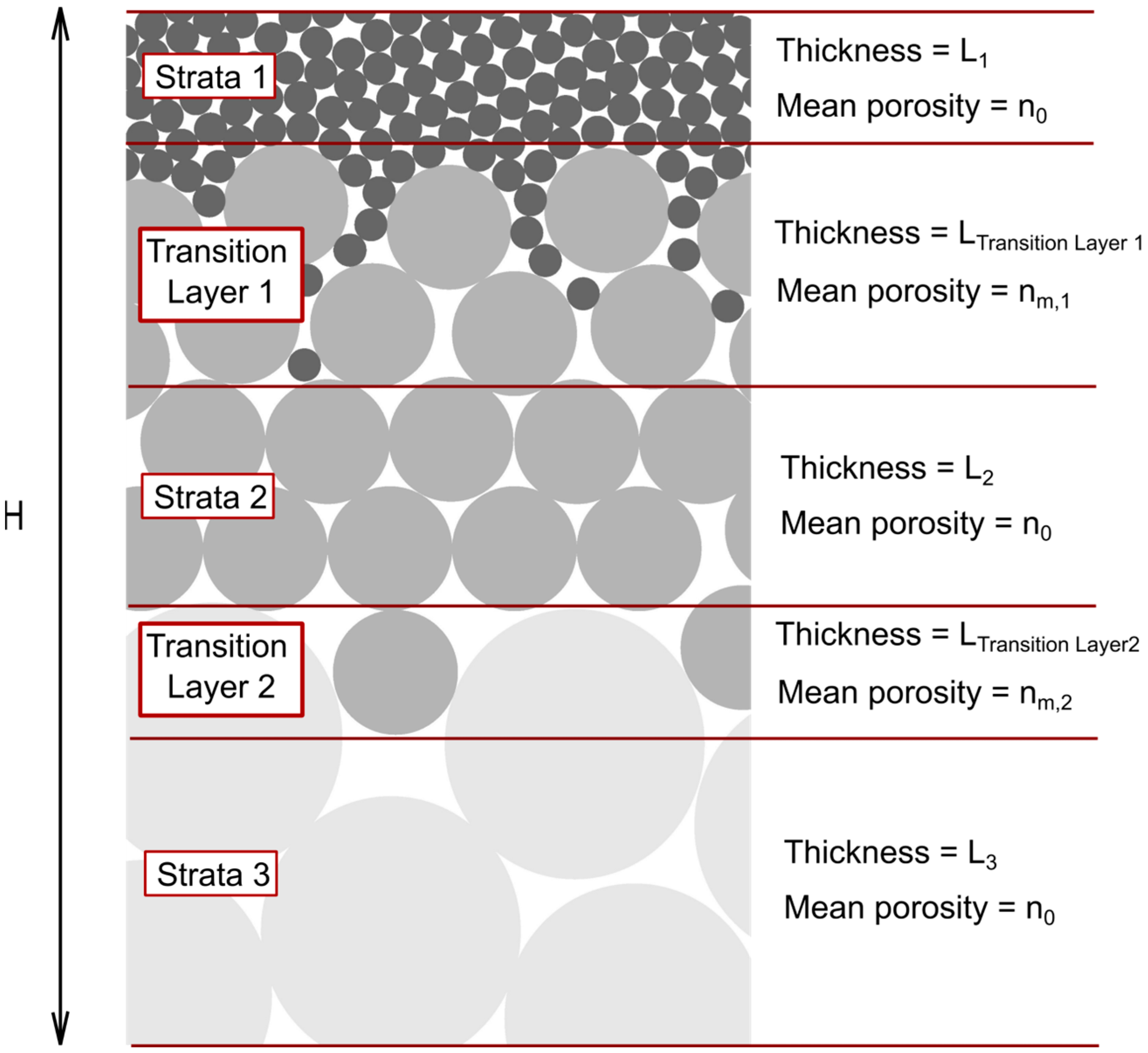
According to [48], a stratified deposit (with layers of different grain sizes) can be divided into two parts: the inhomogeneous transition layer between two neighbouring layers/strata and the homogeneous section of the strata that is unaffected by the intersection (Figure 1). The porosity distribution in the homogeneous section follows that in a uniform sphere packing, which should generally oscillate around a value between 0.36 and 0.4, as introduced above. Within the transition layer, the results of [48] showed that the overall porosity of the sediments has a decreasing and then increasing distribution.
Determining the length of the transition layer and the porosity distribution in it is therefore the key to investigating the porosity value of a layered system. Although the study in [48] gave an empirical relationship between the length of the transition layer and the ratio R of particle size from two neighbouring homogeneous layers, the distribution of porosity within the transition layer was limited to a few laboratory results.
When the upper-layer particles are smaller than those of the base layer—the main focus of this study—the transition layer primarily forms through the infiltration of fine particles into the coarse matrix. Unlike the empirical generalization in [48], ref. [49] provided the first theoretical description of this process, treating fine-sediment infiltration as stochastic. In their P-model, the probability P represents pore bridging by fine sediments, while [50] introduced the β-model, where the trapping coefficient β denotes the fraction of fines retained per unit vertical distance. Assuming constant β and sufficient sediment supply, the steady-state fine-sediment profile follows an exponential form: f = f0·exp (−βz) [51], where f0 is the fine sediment volume fraction at the bed surface and z is the depth.
However, both the P- and β-models have their limitations. The β-model predicts a finite infiltration depth in all cases, conflicting with experiments by [48,52], which showed unbounded infiltration when the size ratio between fine and coarse particles exceeded a critical value. Although the P-model can distinguish between finite and infinite infiltration, it requires accurate estimation of P and temporal evolution of the fine-sediment profile—measurements difficult to obtain experimentally, resulting in limited data. To address these challenges, the present study aims to conduct an empirical analysis of the porosity distribution in the transition layer directly, thereby avoiding the explicit determination of P or β.
It is worth noting that, in addition to the geometric characteristics of sediment particles in the top and base layers, deposition conditions also play a crucial role in the formation of the transition zone. Previous studies (e.g., [53,54]) have shown that higher sediment settling rates and flow-induced shear forces tend to reduce sediment infiltration depth. Furthermore, refs. [55,56] demonstrated that, as rough rock joint surfaces slide—corresponding to the downward infiltration of upper-layer sediments—the aperture and contact areas evolve, thereby altering interparticle flow paths and pressure losses. These hydraulic changes, in turn, affect the mechanical stresses acting on and within the fracture surfaces, potentially modifying the base matrix structure and influencing transition zone development.
The present study focuses primarily on the influence of sediment particle size in the upper and lower layers on the formation of the transition zone. Specifically, we examine cases where the transition zone fully develops under low sediment deposition rates and in the absence of flow-induced shear forces. These conditions provide a baseline for future investigations into the effects of deposition conditions and hydro-mechanical interactions.
This paper is the first in a two-part series. The primary objective of this part is to establish empirical relationships between the thickness of the transition layer (L) and the grain-size ratio (R), as well as between the porosity of the transition layer (nm) and R. Section 2 introduces a calculation model for determining the average porosity of stratified samples. Section 3 outlines the laboratory procedures and measurement methods, Section 4 presents the calibration and validation of the numerical model, and Section 5 provides a discussion of the results.

2. Calculation Model

For a stratified structure with a known total height H, it is assumed that the base-layer sediment is sufficiently thick and that the number of top-layer intruding particles is large enough for each transition layer to fully develop (Figure 2). Since all sediment layers outside the transition zones consist of uniform particle sizes, their porosity n0 lies between 0.36 and 0.4 and is therefore a known quantity. The average porosity of the stratified structure can be calculated using the following formula:
n s t r a t i f i e d = V p o r e V t o t a l = V p o r e ,   L a y e r 1 V t o t a l + V p o r e ,   L a y e r 2 V t o t a l + + V p o r e ,   L a y e r N V t o t a l = A · L 1 · n L a y e r 1 A · H + A · L 2 · n L a y e r 2 A · H + + A · L N · n L a y e r N A · H ,
H = L k .
Vpore,LayerK, nLayerK and LK represent the pore volume, the porosity and the length of Layer K. A denotes the cross-sectional area of a sufficiently large control volume. By classifying the layers into two categories—the transition layers and the homogeneous layers—the following relationship is obtained:
n s t r a t i f i e d = n 0 · H L T r a n s i t i o n _ L a y e r _ i + n m , i · L T r a n s i t i o n _ L a y e r _ i H
Here, L T r a n s i t i o n _ L a y e r _ i and n m , i represent the length of the i-th transition layer and the average porosity of the layer, respectively. By determining the relationships between L T r a n s i t i o n _ L a y e r _ i , n m , i , and the particle size ratio R between top- and base-layer particles, it becomes possible to predict the porosity of a stratified structure based on the particle size arrangement (i.e., ratio R) within the sample solely.

3. Laboratory Experiment

3.1. Methodology

3.1.1. Model Setup and Experiment Procedure

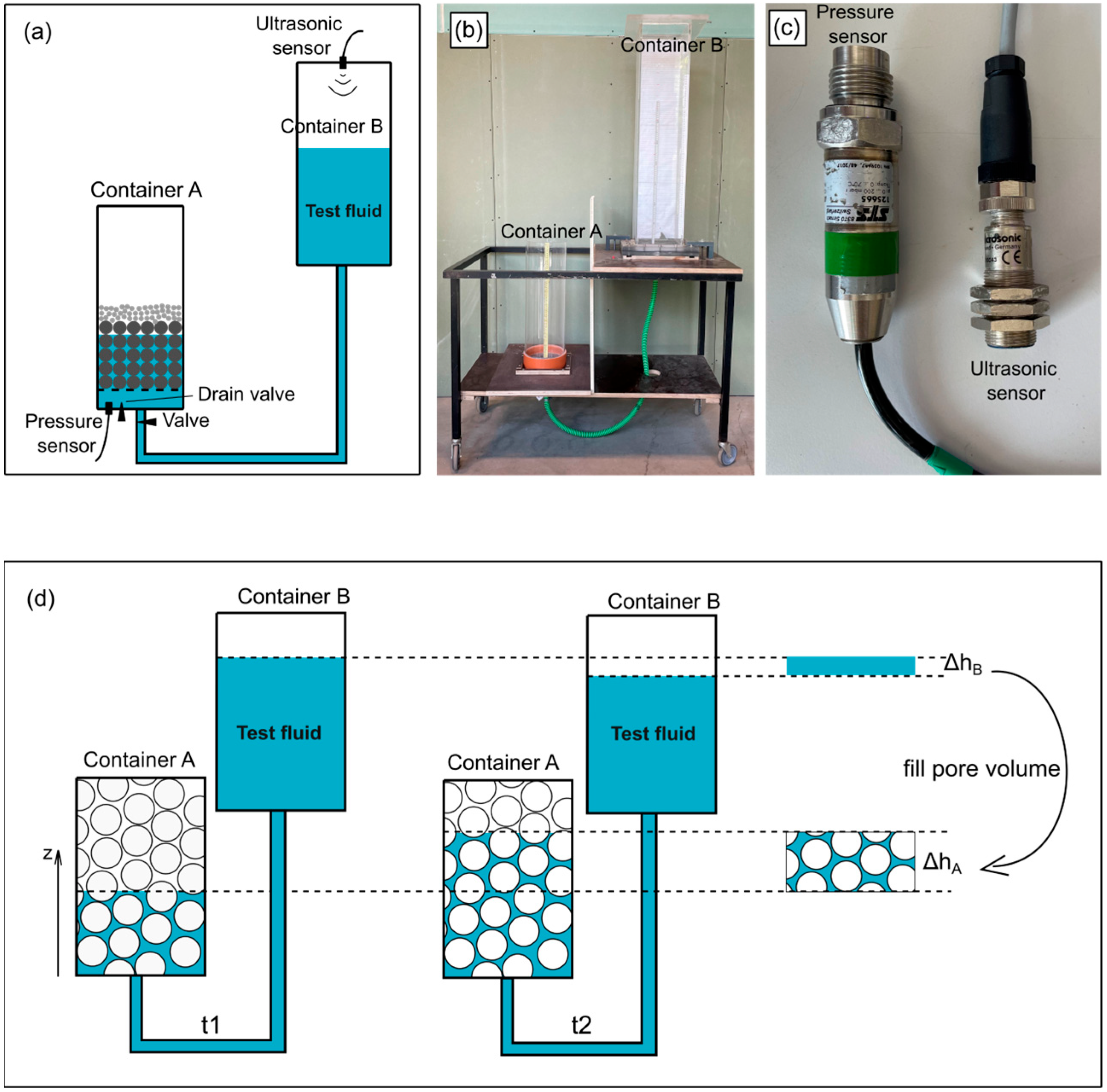
A custom-designed apparatus was developed to measure the vertical porosity distribution in sediment samples. It consists of two interconnected containers (Figure 3a,b). Container A, a cylindrical vessel (20 cm inner diameter, 60 cm height), holds the sample, while Container B, a rectangular reservoir (20 × 20 cm cross-section, 95 cm height), serves as the test fluid supply. During testing, the fluid level in B is maintained above that in A, generating a pressure difference that induces slow flow from B to A. As fluid infiltrates the sample, the corresponding volume change in B represents the pore-filling fluid. Fluid levels in A and B are monitored by a high-sensitivity pressure sensor and an ultrasonic probe, respectively.
The vertical distribution of porosity along the sample height can be calculated using the following equations:
n l o c a l = V p V t = A B · h B A A · h A =   A B · h B / Δ t A A · h A / Δ t =   A B · v B A A · v A ,
n ( z ) = A B · v B ( z ) A A · v A ( z )
Here, AA and AB represent the cross-sectional areas of containers A and B, respectively, while vA and vB denote the rates of fluid level change in containers A and B (Figure 3d).
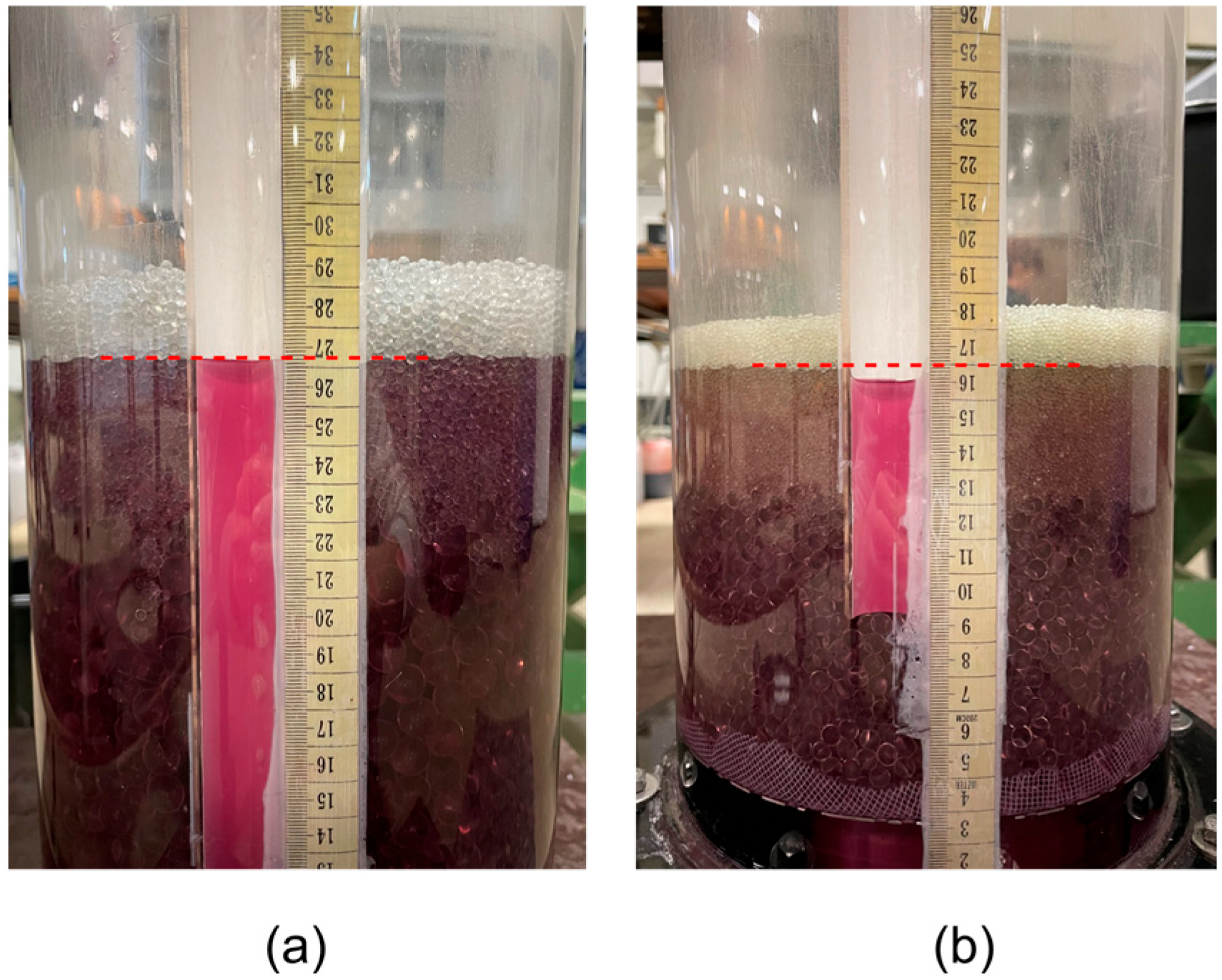
Given the porous nature of the samples, a mixture of water, ethanol, and a surfactant (Polysorbate 20) in a mass ratio of 70:25:5 was used as the test fluid to reduce capillary effects by lowering surface tension. Preliminary tests showed that in samples composed of 3 mm glass beads, the fluid level within the sample rose nearly parallel to that in the pressure tube, indicating negligible capillary influence (Figure 4a). In contrast, samples composed of 1.5 mm beads exhibited a fluid level significantly higher than that in the pressure tube, demonstrating a pronounced capillary effect (Figure 4b). Consequently, only glass beads with diameters ≥ 3 mm were used to prepare the samples in this study.
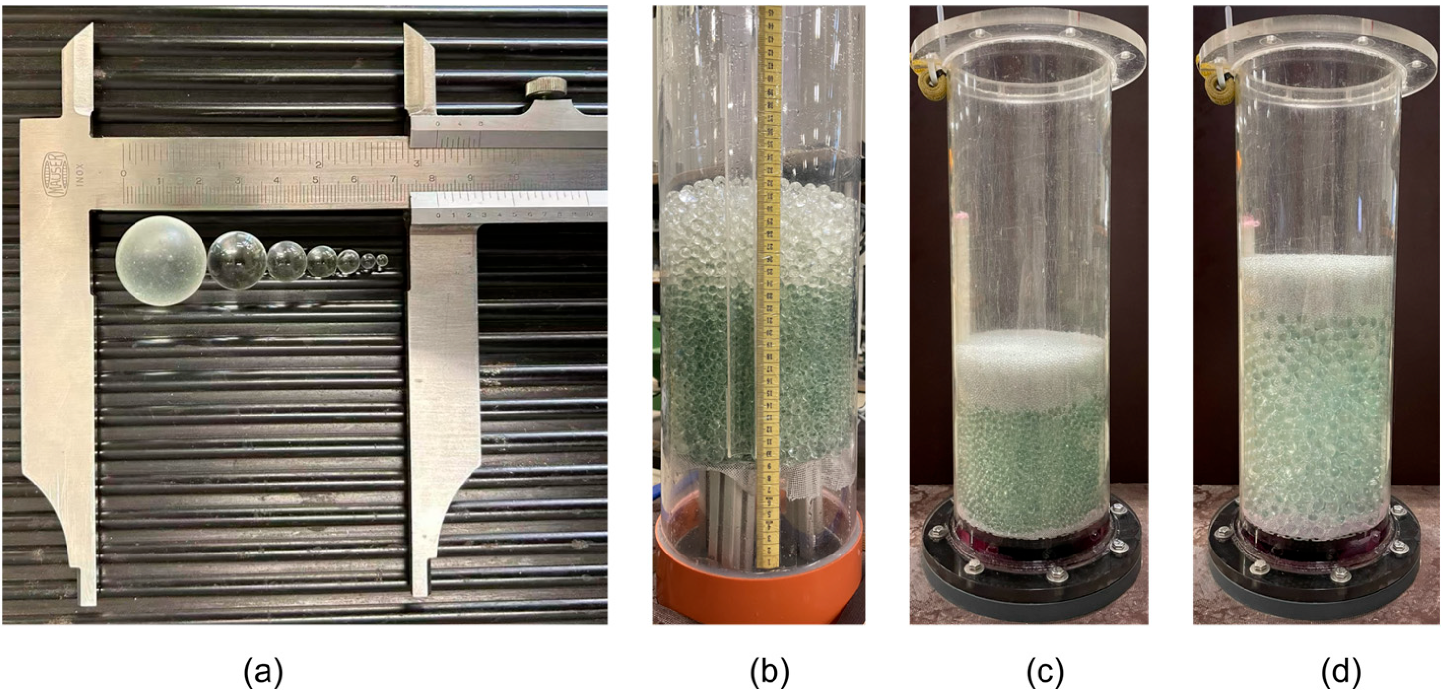
During the laboratory experiments, stratified samples were prepared by sequentially depositing glass beads of different sizes (Figure 5). Two depositional environments were tested: air and pure water. This comparison aimed to examine whether the damping effect of water on particle settling influences the thickness of the transition layer. Although the study primarily focuses on cases where the upper layer is finer than the base layer, several configurations with coarser upper layers were also tested to provide preliminary insights into transition-layer development under inverse stratification.
In-air deposition: The valve between containers A and B (Figure 3a) remained closed. Glass beads of diameter DBase were gently added in portions of approximately 250 g into the dry container A. During deposition, container A was lightly tapped, and the surface was stirred to prevent large pores caused by bridging between beads. When the sediment height reached roughly 20·DBase, deposition was stopped and the surface was leveled without compaction, forming the base layer. Subsequently, glass beads of diameter DTop were added in the same manner to form the top layer. The beads were released close to the sediment surface to minimize settling velocity. During top-layer deposition, container A remained vibration-free, so infiltration of the upper beads into the base layer occurred solely under gravity.
Wall effects arose from the rigid container boundaries, producing locally higher porosity within about five particle diameters of the wall [57]. As the container-to-particle size ratio increased, the relative influence of this effect decreased. Some upper-layer beads were observed to infiltrate through the larger wall-adjacent pores to the base of the sample; the potential impact of this phenomenon on transition-layer measurements is discussed in Section 5.4.
After sample formation, the valve between containers A and B was opened, allowing the test fluid to flow slowly from B to A. Fluid levels were recorded at 10 Hz by a pressure sensor and an ultrasonic probe. The valve was then closed once the sample was fully submerged. Container A was gently tapped to confirm full saturation—no bubbles were observed. The valve opening was adjusted to maintain a slow rise in fluid level (0.05–0.1 cm/s). Each particle-size combination was tested in triplicate under in-air deposition conditions.
In pure water deposition: The valve between containers A and B remained closed. Container A was first filled with pure water, and glass beads of diameters DBase and DTop were sequentially deposited using the same procedure as in the in-air experiments to form a stratified sample under water. After sample formation, the drainage valve at the bottom of container A (Figure 3a) was opened to slowly discharge the water. Pressurized heated gas was then introduced through the drainage outlet, and the sample was dried for 24 h. Once drying was complete, the valve between containers A and B was opened, and the fluid-level changes in both containers were measured using the pressure sensor and ultrasonic probe, following the same procedure as in the in-air deposition tests. Each particle-size combination was tested two to three times under in-water deposition conditions.
The combinations of DBase and DTop used in in-air and in pure water deposition are listed in Table 1:

3.1.2. Data Analysis–Determination of the Transition Layer Length, the Minimum and the Average Porosity Within the Transition Layer

Based on the recorded variations in the test-fluid levels in containers A and B, the rate of fluid-level change in each container was first determined, and the local porosity at different sample heights was then calculated using Equation (5). The length of the transition layer was subsequently obtained by analyzing the porosity distribution along the height. The minimum and average porosities within the transition layer were also derived. The detailed analysis process, illustrated in Figure 6 and Figure 7, is summarized below.
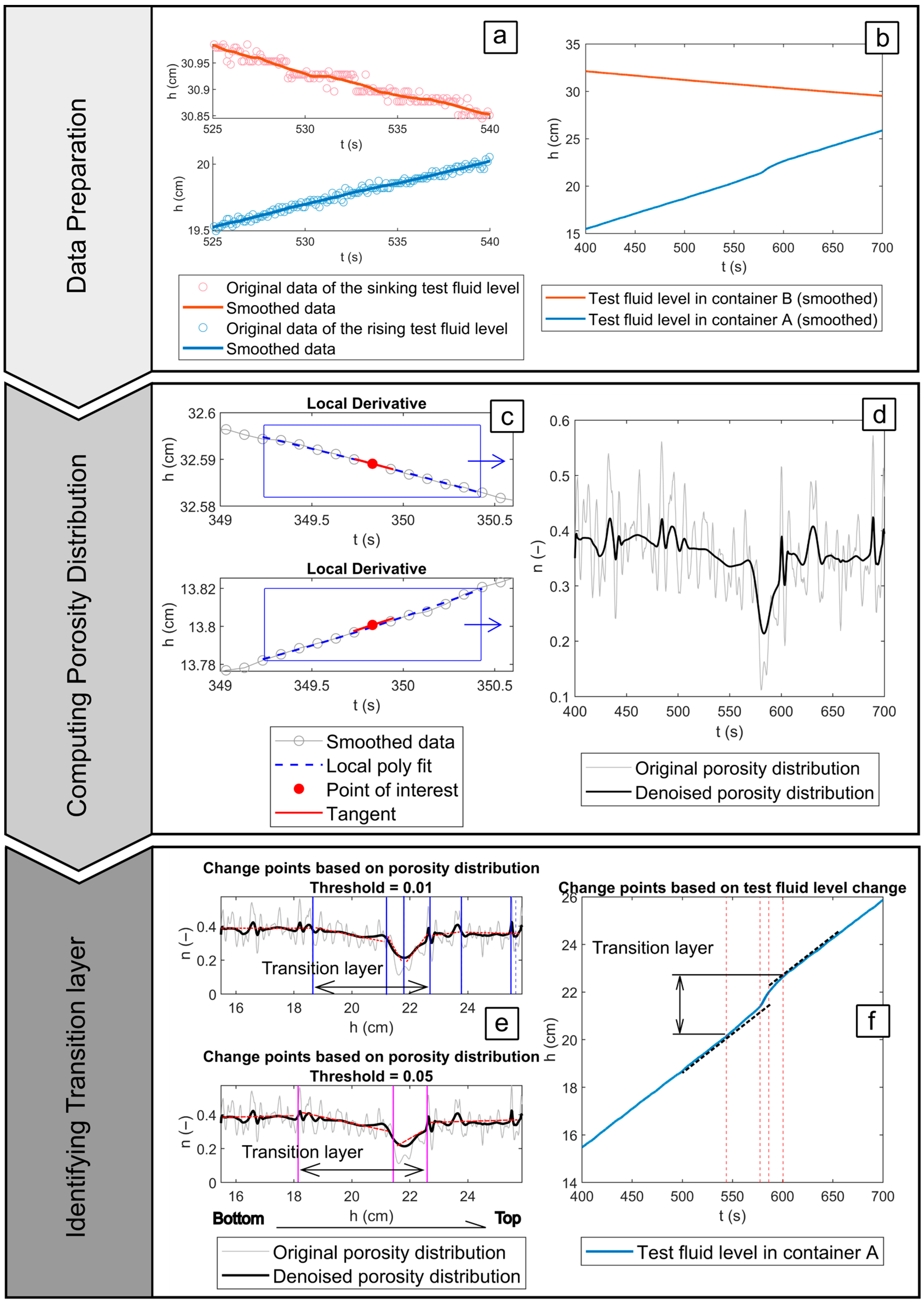
Data preparation: The raw experimental data comprise time series of the fluid levels in containers A and B, where the level in A gradually rises as that in B decreases (Figure 6a). As described in Section 3.1.1, both signals were recorded at 10 Hz using a pressure sensor and an ultrasonic probe. A simple moving average (SMA) was applied to smooth the discrete data, using a sliding window corresponding to a 10 mm fluid-level change (Figure 6b). The mean RMSE between the raw and smoothed data was 0.046 mm, indicating that smoothing did not distort the underlying trend.
Calculating porosity distribution: The rate of fluid-level change was obtained by differentiating the height–time relationship. Because the smoothed data remained discrete, a quadratic polynomial was fitted within a sliding window, and its derivative at the window midpoint was used to calculate the local rate (Figure 6c). From this, the temporal porosity variation n = n(t) was computed using Equation (4) (Figure 6d, gray line). Wavelet denoising was then applied to remove high-frequency noise and retain the main porosity trend (Figure 6d, black line). Given the one-to-one relationship between fluid level and time, the porosity distribution along the height was determined as n = n(h).
Identification of the transition layer: The porosity profile typically decreases from a constant value to a minimum before returning to its initial level (Figure 6e). The deviation from the constant porosity represents the intrusion of top-layer particles into the base layer and thus defines the transition layer. To quantify this region, piecewise linear segmentation [57] was applied to the porosity–height curve. Significant slope changes (“breakpoints”) were identified as the start and end of the transition layer. Because breakpoint detection depends on a user-defined threshold, two independent analysts performed the segmentation under different threshold settings, and the averaged results were used to reduce subjectivity. The same approach was applied to the fluid-level–time curve in container A (Figure 6f). When top-layer particles intrude into base-layer pores, local porosity decreases, accelerating the fluid rise in this area. This behavior produces distinct changes in the slope of the height–time curve, which correspond to the beginning and end of the transition layer. The final transition-layer length was determined by averaging the results from both the porosity–height and fluid-level–time analyses.
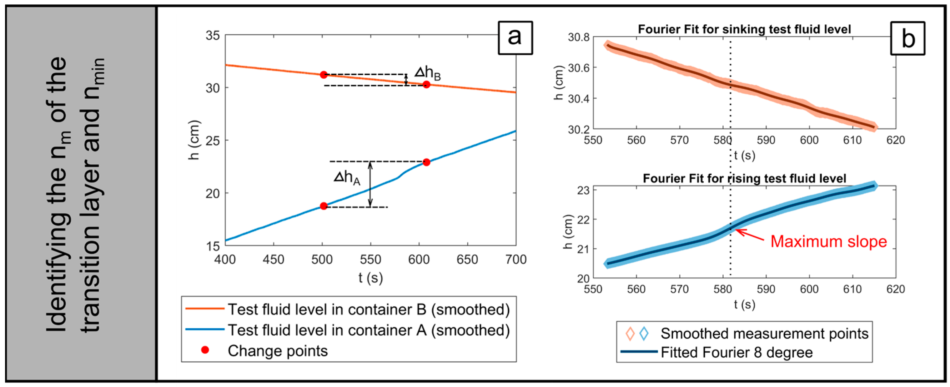
Identification of the minimum porosity and the average porosity within the transition layer: Based on the change points identified in Figure 6e,f, the thickness of the transition layer (ΔhA) was determined (Figure 7a). The corresponding drop in fluid level in container B (ΔhB) represents the volume of test fluid required to fill the pores within this layer. The average porosity was then calculated as nm = (AB·ΔhB)/(AA·ΔhA), where AA and AB represent the cross-sectional areas of containers A and B, respectively.
The local porosity estimation method shown in Figure 6c, which employs a sliding window, is sensitive to measurement noise and can introduce significant uncertainty in identifying the minimum porosity within the transition layer. To improve accuracy, an alternative approach was adopted. Instead of a small sliding window, a fixed window approximately equal to the transition-layer thickness was applied to capture the relevant portion of the fluid-level curve (Figure 7b). A smooth curve was then obtained by fitting the data within this window using a Fourier function. As the minimum porosity occurs at the point of maximum rate of fluid-level rise, differentiation of the fitted function yielded the corresponding rate and thus the minimum porosity (nmin). This method offers two key advantages: it captures the overall trend of fluid-level variation, thereby reducing sensitivity to local noise, and it provides a stable estimate of nmin that is largely independent of the chosen window size, enhancing the robustness of the results.

3.1.3. Principle of Reliability Assessment of Measurement Results

Evaluation of Porosity Measurements: Since the method for determining the transition-layer length relies on the sample’s porosity distribution, the accuracy of porosity measurements—serving as the fundamental dataset—directly affects the reliability of the results. As noted in Section 1, the porosity of randomly packed uniform spheres typically ranges between 0.36 and 0.40, which provides a useful benchmark for identifying significant deviations in measured values. Furthermore, wall effects cause porosity near the container walls to be higher than at the center, making the measured porosity dependent on the ratio of container diameter to particle diameter [27]:
n = n 0 · e D G r a i n D C o n t a i n e r .
Here, n is the measured porosity value, and n0 is the porosity measurement in an infinitely large container. DGrain and DContainer represent the diameters of the spheres and the measurement container, respectively. The inner diameter of container A (DContainer) used in this experiment was fixed at 20 cm, while the diameters of the glass spheres (DGrain) varied from 3 mm to 20 mm. Excluding the transition layer (Figure 6e), the porosity corresponding to each DGrain was determined from the stable segments of the porosity distribution. Owing to the range of DGrain values, porosity measurements were obtained for various DGrain/DContainer ratios. These results were then compared with Equation (6) to evaluate the reliability of the measured porosity data.
Evaluation of Transition Layer Length Measurements: The measured transition layer lengths for each particle size combination are first nondimensionalized:
R =   D B a s e D T o p ,
φ T = L T r a n s i t i o n _ l a y e r D B a s e .
Here, DBase and DTop represent the diameters of the base- and top-layer spheres, respectively, and LTransition_layer denotes the transition layer length. The reliability of the measured transition layer lengths is evaluated by comparing the results of this study with the φTR distribution reported by [48].

3.2. Results of Laboratory Research

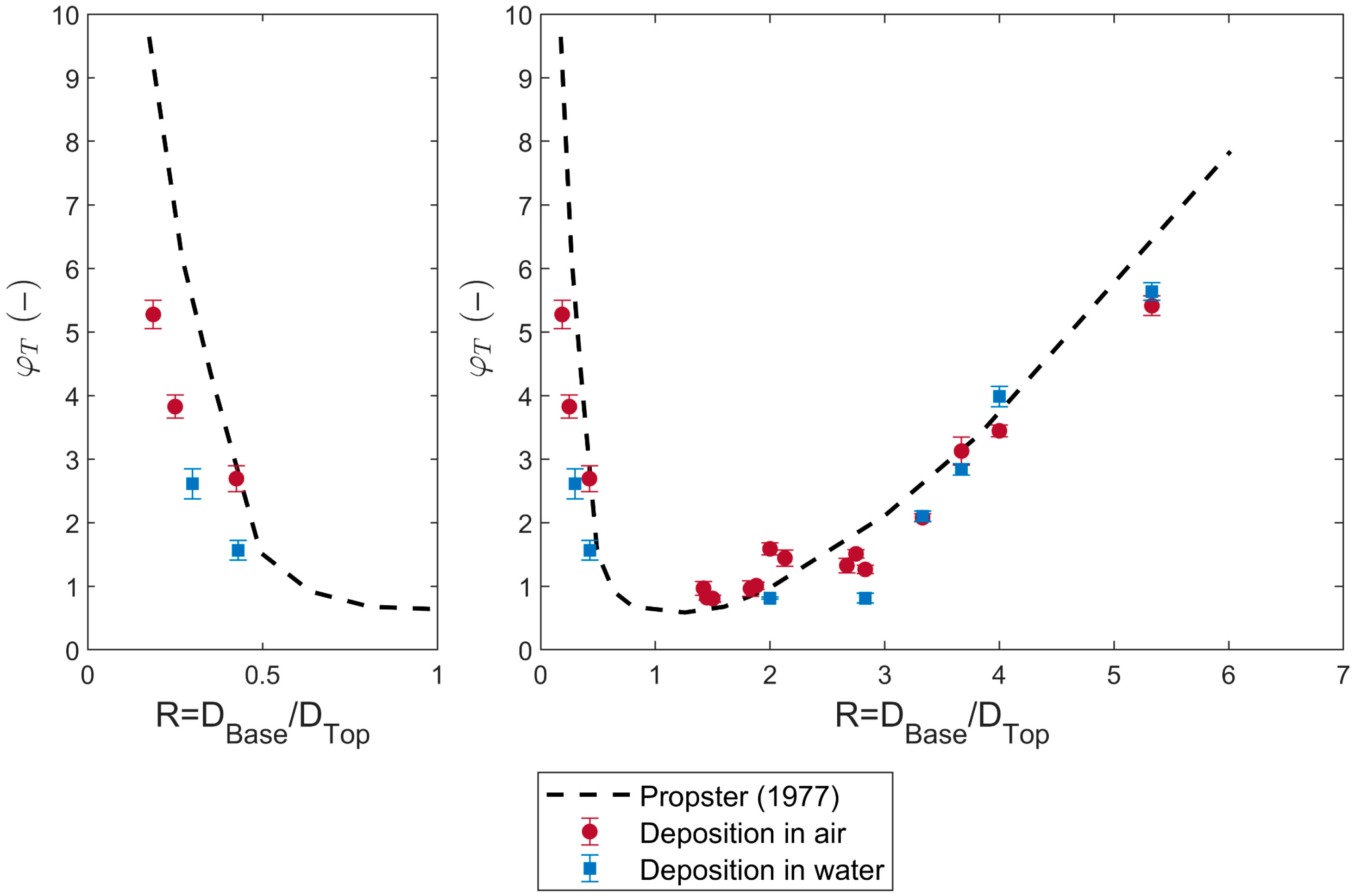
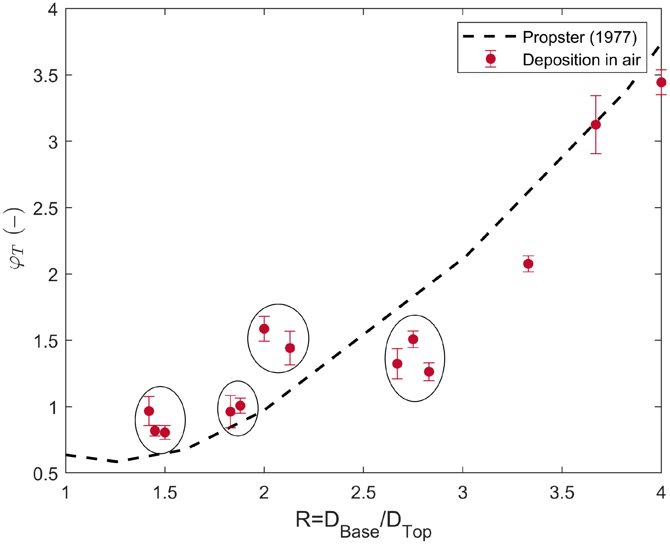
Figure 8 shows the relationship between the dimensionless transition layer length φT (=LT/DBase) and the grain-size ratio R between the top- and base-layer particles.
Deposition in air: When R is greater than 0 but less than 1, the top-layer particles are larger than the base-layer particles. In this case, the top-layer particles are unable to infiltrate the base layer. The transition layer forms primarily due to the disturbance of the base-layer surface caused by the larger top-layer particles [48]. As the size difference between the top- and base-layer particles decreases, the transition layer becomes progressively thinner. Compared to the experimental results of Propster [48], the transition layer lengths measured under dry conditions in this study are significantly shorter—by up to 35%.
When R exceeds 1, the top-layer particles are smaller than the base-layer particles and can infiltrate downward. The transition layer length in this regime is directly related to the downward penetration depth of the top-layer particles. As R increases, the infiltration capacity of the top-layer particles improves, and the measured transition layer length increases accordingly. For R values below 4, the measurements from this study closely match the results of [48]. However, as R increases further, the transition layer lengths obtained in this study tend to be slightly lower than those reported by [48], with deviations around 15%.
Comparison between in-air and in water deposition: When R is greater than 0 but less than 1, the transition layer formed in water is nearly 40% shorter than that formed under dry conditions.
When R exceeds 1, the influence of water on the penetration depth of the top-layer particles appears to diminish with increasing R. For R values below 3, the transition layer length formed under in-water deposition remains approximately 40% shorter than that under in-air conditions. However, when R exceeds 3, no significant difference is observed between the transition layer lengths formed under in-air and in-water deposition.
In different ranges of the R value, water appears to have varying effects on the formation of the transition layer, which will be discussed in detail in Section 5.5.
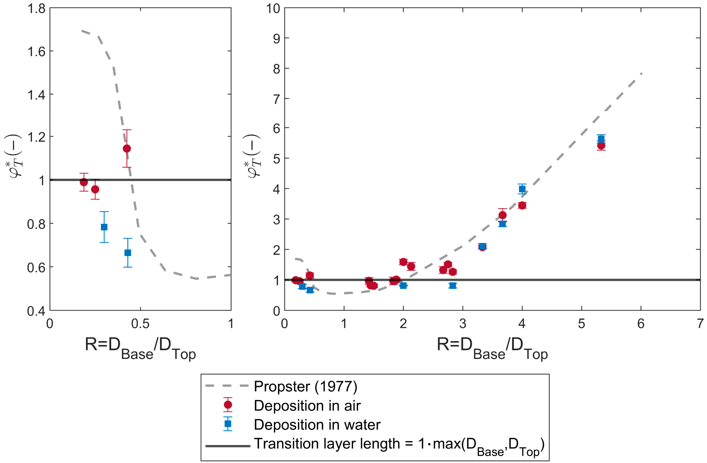
In Figure 9, to more clearly illustrate the embedding depth of top-layer coarse particles into the base-layer fines when R < 1, the dimensionless transition layer length φ*T (=LT/max(DBase, DTop) is recalculated. This adjustment does not affect the values for R > 1. For R < 1, φ*T = 1 corresponds to the full embedding of a single top-layer particle into the base-layer deposit. Results show that, under both in-air and in-water deposition, the embedding depth of top-layer particles remains limited when R < 1—typically no more than the diameter of a single particle. Although the experiments of [48] reported slightly deeper embedding at the same R, the depth still does not exceed two top-layer particle diameters.
Error analysis: by averaging the results from different analysts and repeated experiments at the same R values, the error in the φT values determined using the piecewise linear segmentation method presented here ranges from 0.04 to 0.22, with an average error of 0.12. Error bars corresponding to each R value are shown in Figure 8 and Figure 9. Although the piecewise linear segmentation method involves some subjectivity, the measurements from different analysts remain largely consistent.
Reliability assessment: In Figure 10, the porosity values of uniform samples composed of spheres with different diameters in a 20 cm diameter cylindrical container are compared with the experimental data from [27]. It can be observed that, besides all measured porosities falling within the theoretical range of 0.36 to 0.40, the decreasing trend of porosity with decreasing DGrain/DContainer ratio aligns well with Frings’ model. This confirms the accuracy of the porosity measurements as the foundational data for determining φT.
Moreover, the trend of φT versus R measured under dry conditions in Figure 8 (especially for R between 1 and 4) largely agrees with the existing data from [48], indicating that significant systematic errors in φT measurements can be essentially ruled out. Differences observed between laboratory results and those from [48] for R less than 1 and greater than 4 are considered to be attributed to variations in particle deposition methods and transition layer length determination approaches between the two studies; this will be discussed in detail in Section 5.2.

4. Numerical Simulation

A key limitation of the laboratory method is its inability to resolve the internal structure of the samples in detail. In contrast, numerical simulations provide access to the coordinates of every individual sphere within the packed structure, enabling detailed internal analysis of the sediment. On this basis, a DEM-based numerical model was calibrated and validated against the laboratory results, and subsequently employed to extend the experimental dataset. During this phase, the numerical simulations considered only cases in which the top-layer particles were smaller than those of the base layer.

4.1. Methodology

4.1.1. Particula 1.3

A simulator tool for computational rock physics of granular materials, Particula 1.3 [58], is a simulation tool designed for computational rock physics, particularly focusing on granular media. It employs the Discrete Element Method (DEM) [59,60] to model the mechanical behavior of granular assemblies, such as sediments and rock formations. The simulation framework encompasses three fundamental components: contact detection, contact resolution, and time-step integration.
Contact Detection: Particula 1.3 uses a two-phase approach for contact detection: the broad phase rapidly filters potential contact pairs using spatial partitioning [61], while the narrow phase performs precise geometric checks. To ensure robustness, especially for fast-moving particles, Particula 1.3 employs continuous collision detection (CCD) to anticipate and handle imminent contacts [58].
Contact Resolution: Particula 1.3 employs an impulse-based contact resolution method (e.g., [62,63]). Instead of resolving contact forces over time, this approach computes instantaneous impulses to enforce momentum conservation and non-penetration constraints at each contact point. The rigid body contact model and discretization used have been described in [58,64,65]. A brief summary is provided here:
For two contacting particles A and B, the relative velocity at the contact point is:
v r e l = v B + ω B × r B ( v A + ω A × r A ) .
v and ω are linear and angular velocity. r is the contact radius vector from the center of mass of a particle to the contact point.
The normal impulse J n is computed to eliminate the normal component of the relative velocity while accounting for restitution e (coefficient of restitution):
J n = ( 1 + e ) ( v r e l · n ) 1 m A + 1 m B + n · [ ( I A 1 ( r A × n ) ) × r A + ( I B 1 ( r B × n ) ) × r B ]
n is the contact normal vector, perpendicular to the contact surface at the point of contact.
Friction is handled by computing a tangential impulse J t that opposes the tangential velocity component and is clamped by Coulomb’s friction limit:
J t   μ J n
μ is the friction coefficient. The total impulse J =   J n + J t is then applied to update the linear and angular velocities of both particles:
v A , n e w = v A J m A ,     ω A , n e w = ω A   I A 1 r A × J
v B , n e w = v B + J m B ,     ω B , n e w = ω B + I B 1 r B × J
m denotes the mass of a particle. To resolve multiple simultaneous contacts, Particula 1.3 uses an iterative solver, which sequentially processes each contact pair and loops over all pairs for several iterations (typically fewer than 10) until convergence [65]. This approach enables efficient and stable simulation of dense granular systems with large time steps.
Time-Step Integration: Particula 1.3 employs a semi-implicit Euler integration scheme, which is well-suited for impulse-based simulations of rigid bodies. This method provides better numerical stability than the explicit Euler method, especially when handling stiff contact conditions or large time steps [66].
After resolving all contact impulses, particle velocities are updated, and then positions are advanced:
v t + t =   v t +   F e x t m t ,                                   ω t + t =   ω t +   I 1 τ e x t t
x t + t = x t + v t + t t ,                       q t + t = n o r m a l i z e ( q t + 1 2 ω t + t · q t · t )
F e x t and τ e x t are external forces (e.g., gravity) and torques. I is the inertia tensor. x and q are position and orientation quaternion. Angular motion is integrated via quaternion rotation.

4.1.2. Simulation Setup

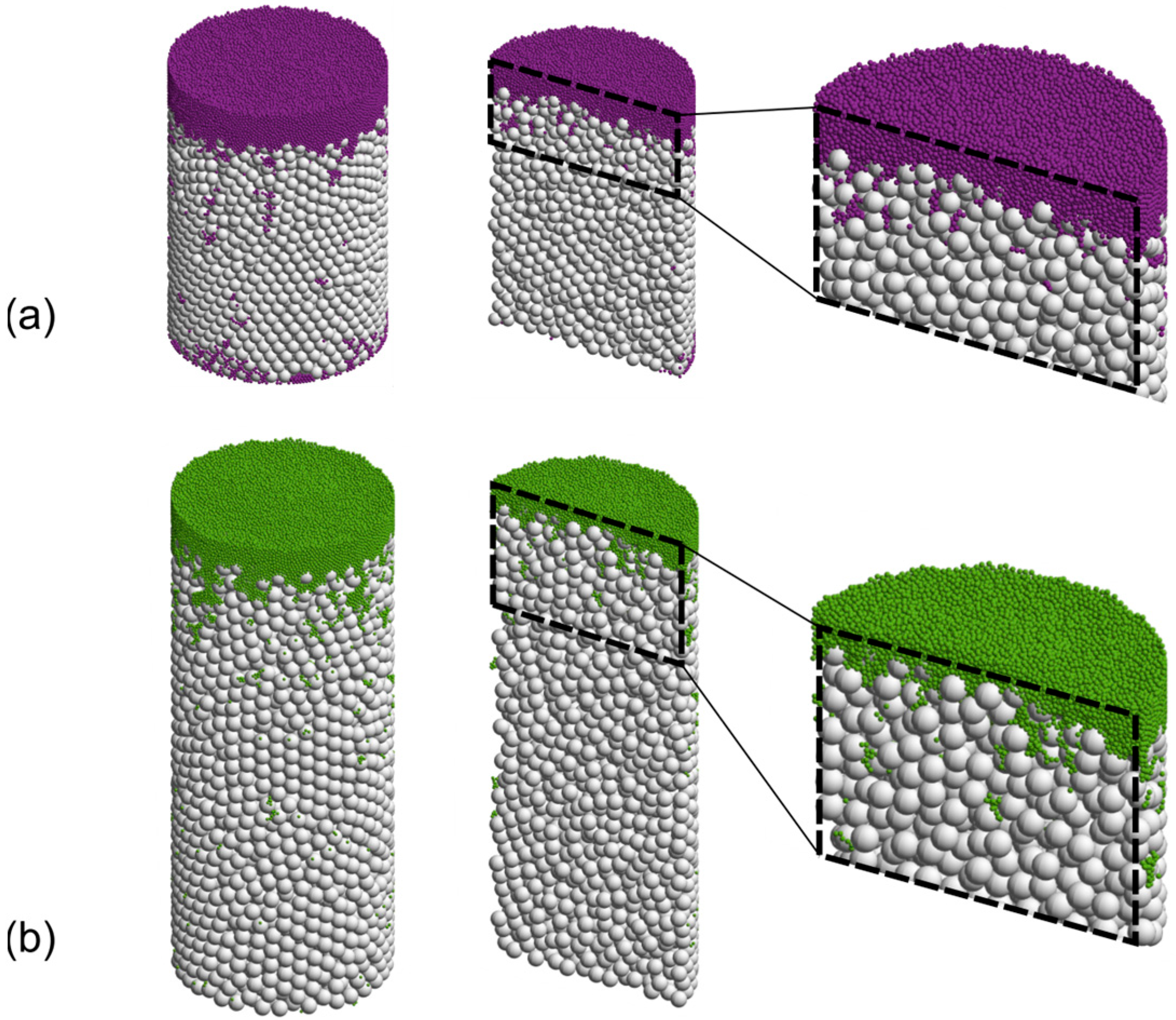
Consistent with the laboratory experiments, the numerical simulations produced stratified samples with a diameter of 20 cm by sequentially depositing spheres of different sizes into a cylindrical container (Figure 11). Particles settled freely under gravity, and their collisions—with other particles and with the container walls—and the resulting motions were computed using Equations (9)–(15). To achieve a dense base layer, vibrations were applied during the deposition of base-layer particles, whereas this vibration mode was deactivated during top-layer deposition to replicate the laboratory conditions.
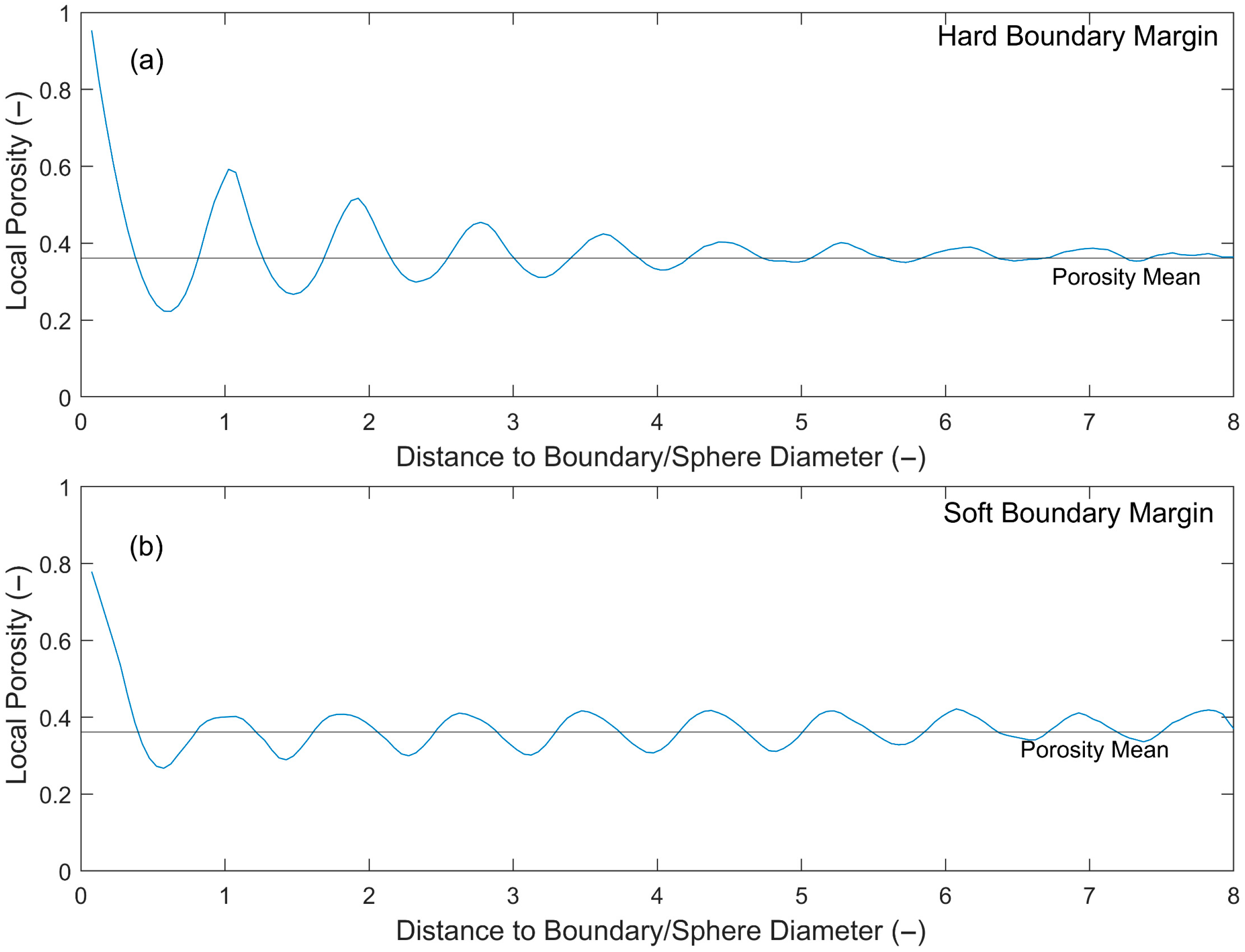
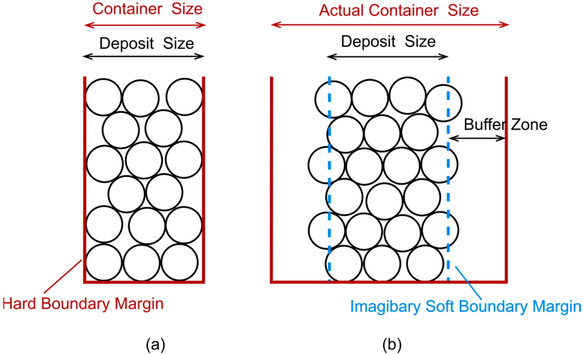
Particula 1.3 supports two boundary condition types: hard and soft boundaries, which are implemented by specifying different buffer-zone lengths. The buffer zone refers to a peripheral region of the model where particle deposition is restricted. When the buffer-zone length is set to zero, the deposit is in direct contact with the container wall. Under this condition, wall effects lead to locally elevated porosity within approximately five particle diameters from the boundary—consistent with the laboratory setup. When the buffer-zone length is greater than zero, particles do not contact the wall directly; instead, their outer arrangement is unconstrained, as if particles could partially pass through an imaginary boundary during deposition (Figure 12). This soft boundary condition substantially reduces the region influenced by wall effects (Appendix A).
In this study, different boundary conditions were applied in two distinct stages of the numerical simulations:
Model Calibration and Validation: At this stage, the numerical simulations replicated the in-air deposition experiments described in Section 3.1.1. Hard boundary conditions were applied to match the experimental setup, and the resulting layered deposits were cylindrical with a diameter of 20 cm.
The porosity distribution of each simulated sample was then extracted (see Section 4.1.3 for details). To ensure consistency in data processing, the piecewise linear segmentation method introduced earlier was applied to the porosity–height profiles, enabling direct comparison between experimental and simulated results.
Because the initial particle positions in the simulations were randomly generated, the deposition process was subject to stochastic variability. Accordingly, three replicate simulations were performed under identical conditions for each case to ensure statistical reliability.
Extension of Experimental Data: In this stage, numerical simulations were used to extend the limited set of experimental data by introducing a broader range of particle size ratios between the base and top layers, defined as R = DBase/DTop. The extended dataset enabled detailed investigation of the relationship between R and key transition layer properties, including the transition layer thickness φT, the average porosity of the transition layer nm, and the minimum porosity within the transition layer nmin. Additionally, the critical value of R′ corresponding to the onset of unlimited percolation of upper-layer particles was explored.
During this stage, cylindrical samples with a diameter of 20 cm were generated under soft boundary conditions. To eliminate the influence of wall effects, a central core with a diameter of 10 cm was extracted from each sample for analysis. An improved method for determining the length of the transition layer was employed (see Section 4.1.3), which enhanced objectivity and efficiency in data processing. Three repeated simulations were conducted for each set of conditions to account for stochastic variability.
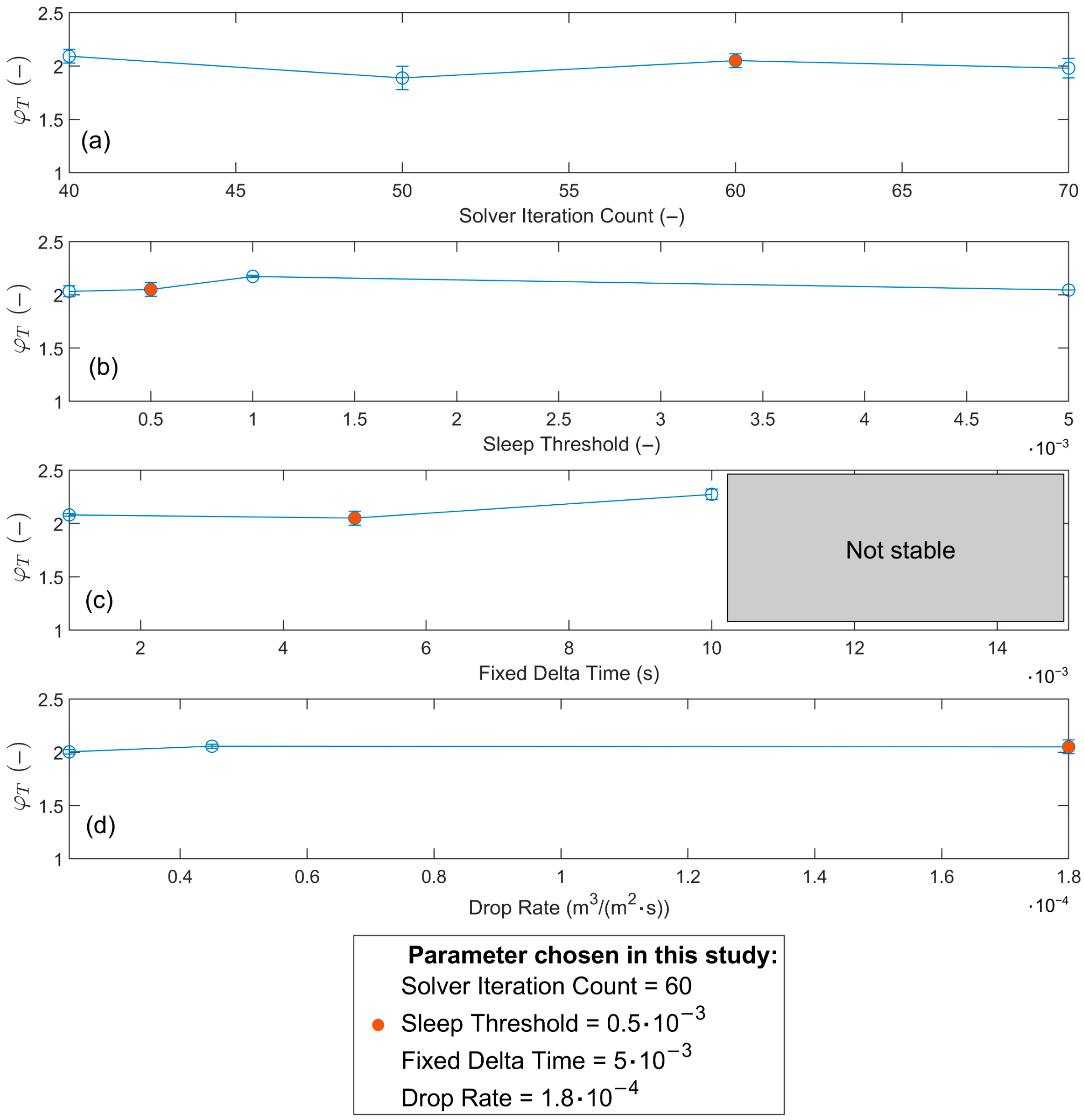
The simulation parameters used are summarized in Table 2. These parameters were determined based on a separate sensitivity analysis (Appendix B). The particle size ratios used in the experimental data extension and friction coefficient effect stages are listed in Appendix C.

4.1.3. Data Analysis—An Improved Method for the Identification of the Transition Layer

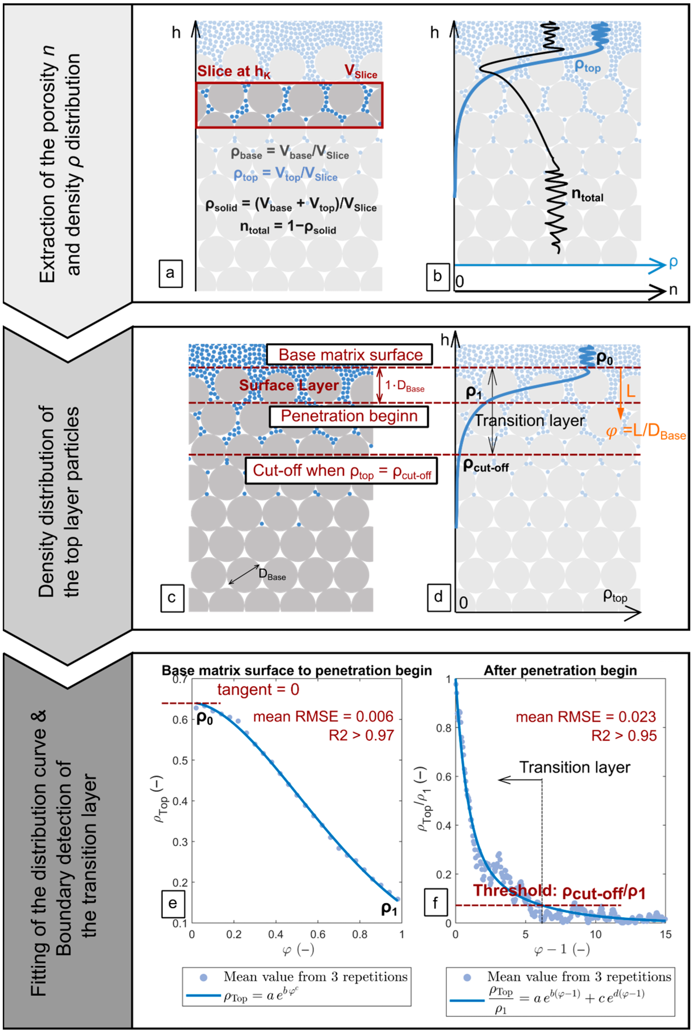
Determination of the transition-layer thickness using piecewise linear segmentation involves a degree of subjectivity. While employing multiple analysts can reduce this effect, it substantially decreases data-processing efficiency. Capitalizing on the ability of numerical simulations to provide the spatial coordinates of individual particles, a more objective and efficient method for determining the transition-layer thickness was developed. The procedure is illustrated in Figure 13.
Porosity and Density Distribution Extraction: The stratified samples generated in the numerical simulations were cylindrical in shape. The sample was divided along the vertical axis into a series of thin slices (Figure 13a), each with a thickness of min(DBase, DTop)/50. For each slice, the volume fractions of top- and base-layer particles were calculated separately to obtain their respective local densities, ρTop and ρBase. The sum of these densities represents the total solid density, ρs, and the local porosity was computed as ntotal = 1 − ρs. This yielded the porosity distribution along the sample height (black line in Figure 13b).
In addition, the height-dependent distribution of ρTop was extracted. For clarity, density rather than porosity was used to describe the top-layer particles, as the gradual decrease in ρTop with depth directly reflects the diminishing presence of intruding particles within the base layer (blue line in Figure 13b).
Improved Method for Determining the Transition Layer: Consistent with the β-model predictions introduced in Section 1, the density of top-layer particles (ρTop) decreases with increasing penetration depth (Figure 13b). The core concept of the improved method is to define a density threshold, ρcut-off. When ρTop falls below this threshold, the proportion of penetrating particles becomes sufficiently small that their influence on the total porosity can be neglected. The height corresponding to ρcut-off is therefore regarded as the lower boundary of the transition layer, while the upper boundary corresponds to the highest point of the base-layer particles (i.e., the base-matrix surface; Figure 13c,d).
In practical implementation, the ρTop distribution is divided into two segments by a user-defined “penetration-begin” line: (i) from the base-matrix surface down to the penetration-begin line, and (ii) below this line (Figure 13c,d). The density data in each segment are then fitted with smooth functions to describe the distribution trends (Figure 13e,f). The rationale for defining a penetration-begin line and applying curve fitting is as follows:
Curve fitting: As shown in Figure 13f, the discreteness of the top-layer particle density distribution increases markedly with penetration depth. Direct application of a density threshold to such discrete data would make the determination of the transition-layer lower boundary highly sensitive to noise. By fitting a smooth curve to the data, this method focuses on the overall trend of density variation with depth while minimizing the influence of random local fluctuations in porosity on transition-layer identification.
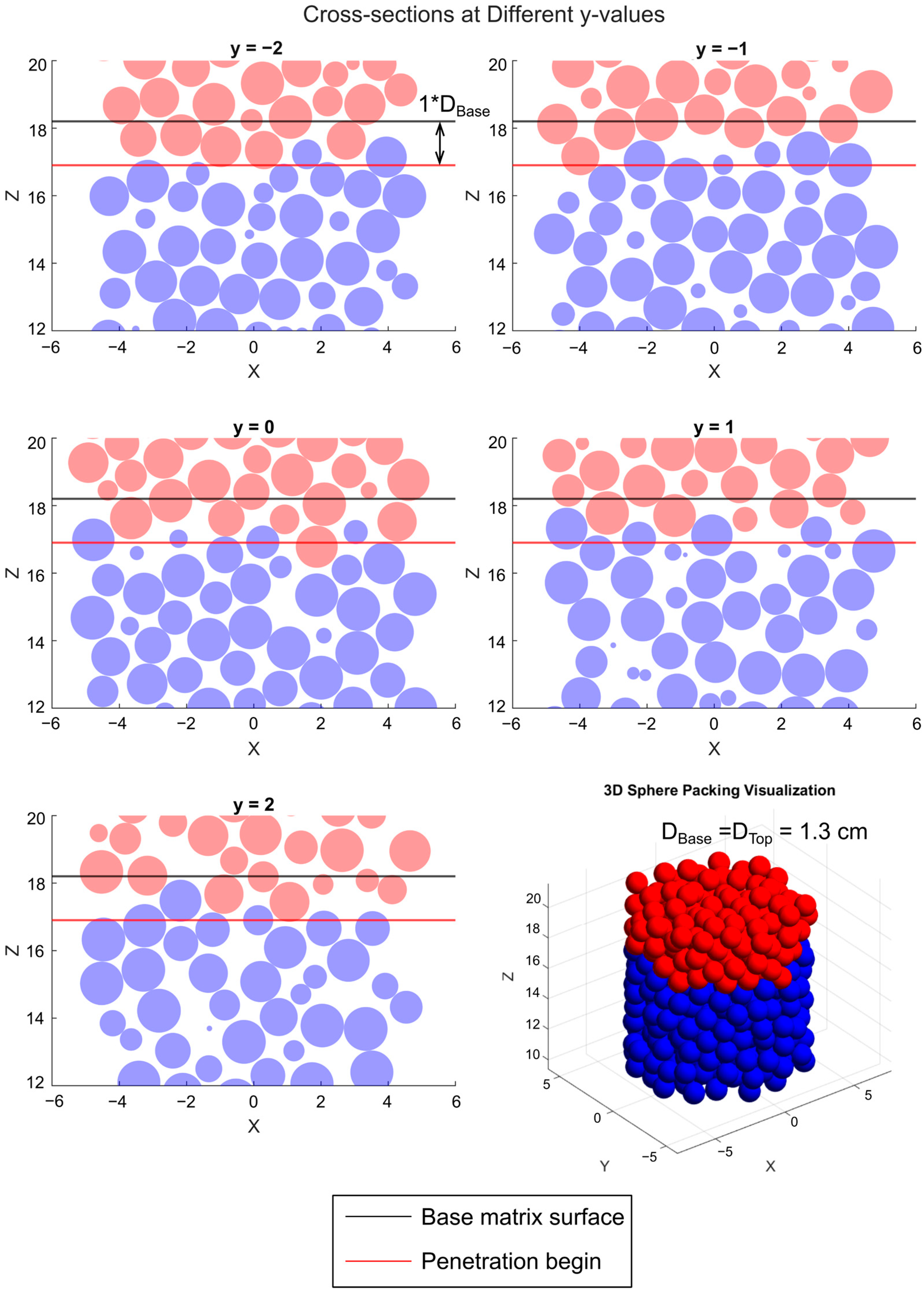
Penetration begins: Repeated tests revealed that a single exponential function cannot adequately represent the entire ρTop distribution. The density of top-layer particles decreases rapidly within approximately 1·DBase below the base-matrix surface, followed by a much slower decline. Preliminary results (Appendix D) indicate that even when DBase = DTop, top-layer particles can still move slightly below the base-matrix surface and accumulate within a region roughly equal to 1·DBase, but they do not penetrate deeper. On this basis, a surface layer is defined as the zone extending from the base-matrix surface to a depth of 1·DBase, where the packing of base-layer particles is relatively loose and larger top-layer particles can accumulate. Below this zone, porosity decreases, and only smaller top-layer particles can penetrate further. The lower boundary of the surface layer is therefore defined as the penetration-begin line.
The density distribution of top-layer particles within the region from the base matrix surface to the penetration begin line follows a compressed exponential distribution (R2 > 0.97, mean RMSE = 0.006):
ρ T o p = a · e b · φ c ,
φ = I n f i l t r a t i o n   D e p t h   f r o m   B a s e   M a t r i x   S u r f a c e D B a s e .
Here, ρTop represents the density of top-layer particles at a given depth, and φ denotes the dimensionless penetration depth (Figure 13d).
Below the penetration begin line, the density distribution of top-layer particles follows a second-order exponential function (R2 > 0.95, mean RMSE = 0.023):
ρ T o p ρ 1 = a · e b · ( φ 1 ) + c · e d · ( φ 1 ) .
Here, ρ1 denotes the density of top-layer particles at the penetration beginning line (Figure 13d). Equations (16) and (18) do not share the parameters a, b, and c.
Using Equations (16) and (18), this study tested three different density thresholds—0.01, 0.02, and 0.03—to determine the lower boundary of the transition layer. Compared to the porosity of uniform spheres (0.36), these thresholds correspond to physical implications where the influence of the penetrating top-layer particles on the local porosity reduction is about 3% (=0.01/0.36), 5% (=0.02/0.36), and 8% (=0.03/0.36), respectively. The transition layer lengths determined by this method were then compared with those derived from the laboratory experiments using the piecewise linear segmentation method.

4.2. Results of Numerical Simulations

4.2.1. Model Calibration and Validation

The first phase of the numerical simulation adopted the same experimental conditions as the laboratory in-air deposition experiments. The transition layer length was determined using the same piecewise linear segmentation method to maintain consistency with the laboratory data processing approach.
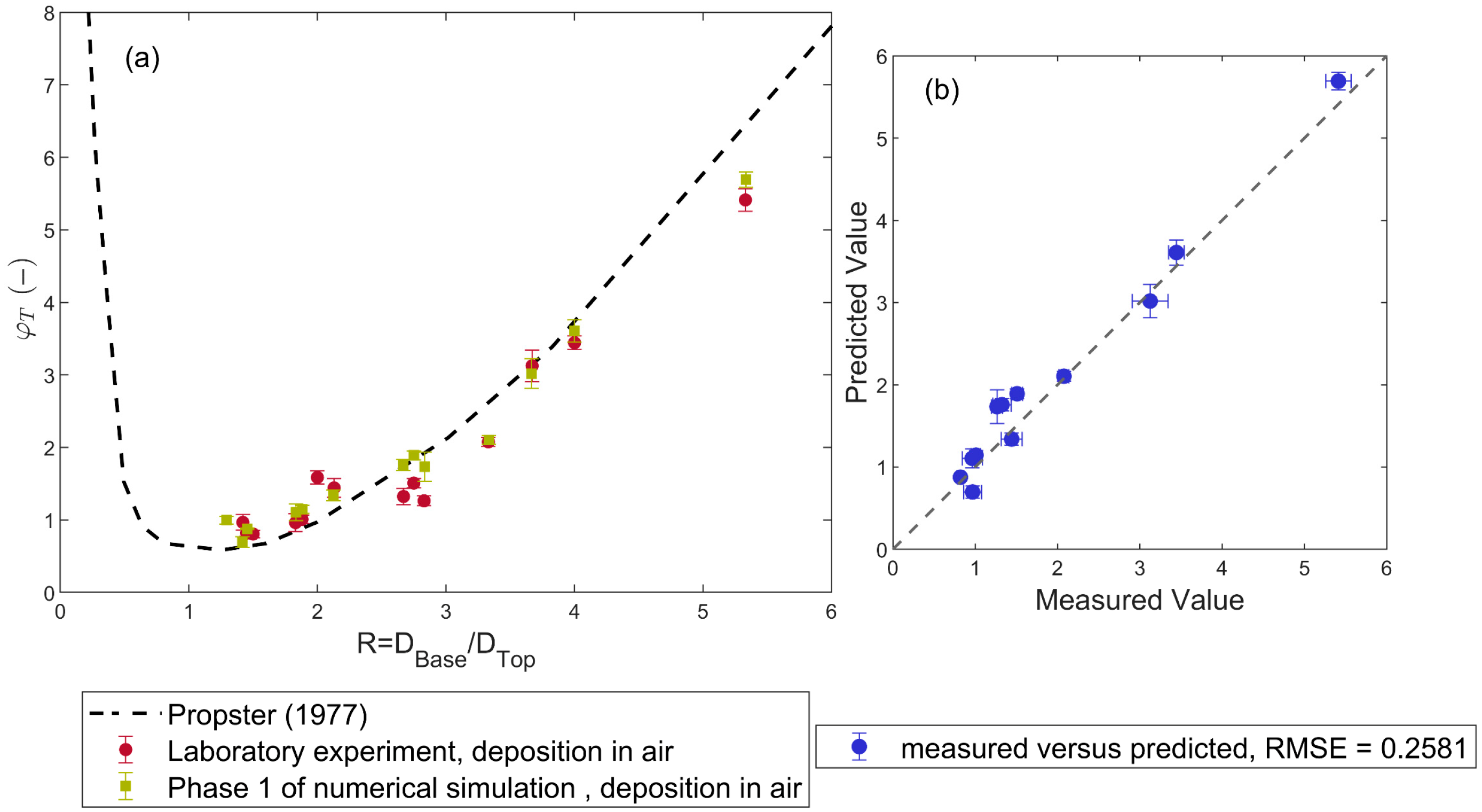
In Figure 14, results from the numerical simulation and laboratory experiments are compared. During the first phase of the simulation, three repeated experiments were conducted for each R value, with error bars representing the uncertainty of transition layer length measurements shown in Figure 14. The measurement errors range from 0.01 to 0.20, with an average error of 0.09. This small error indicates a high consistency among the three simulation repetitions for the same R value, effectively ruling out randomness as a factor influencing the results.
As shown in Figure 14, the φTR trend observed in the numerical simulation nearly overlaps with the laboratory results. The RMSE between the simulation predictions and laboratory measurements is 0.26. Based on the results of the preliminary calibration and validation, the Particula 1.3 software is considered to be capable of reproducing laboratory experiments and thus can be used to extend the existing laboratory data.

4.2.2. Comparison of the Two Different Methods for the Transition Layer Identification

During the second phase of the numerical simulations, a wider range of stratified samples with different R values was produced. The accuracy and efficiency of the improved density-threshold method (Section 4.1.3) were assessed and compared against those of the conventional piecewise linear segmentation method.
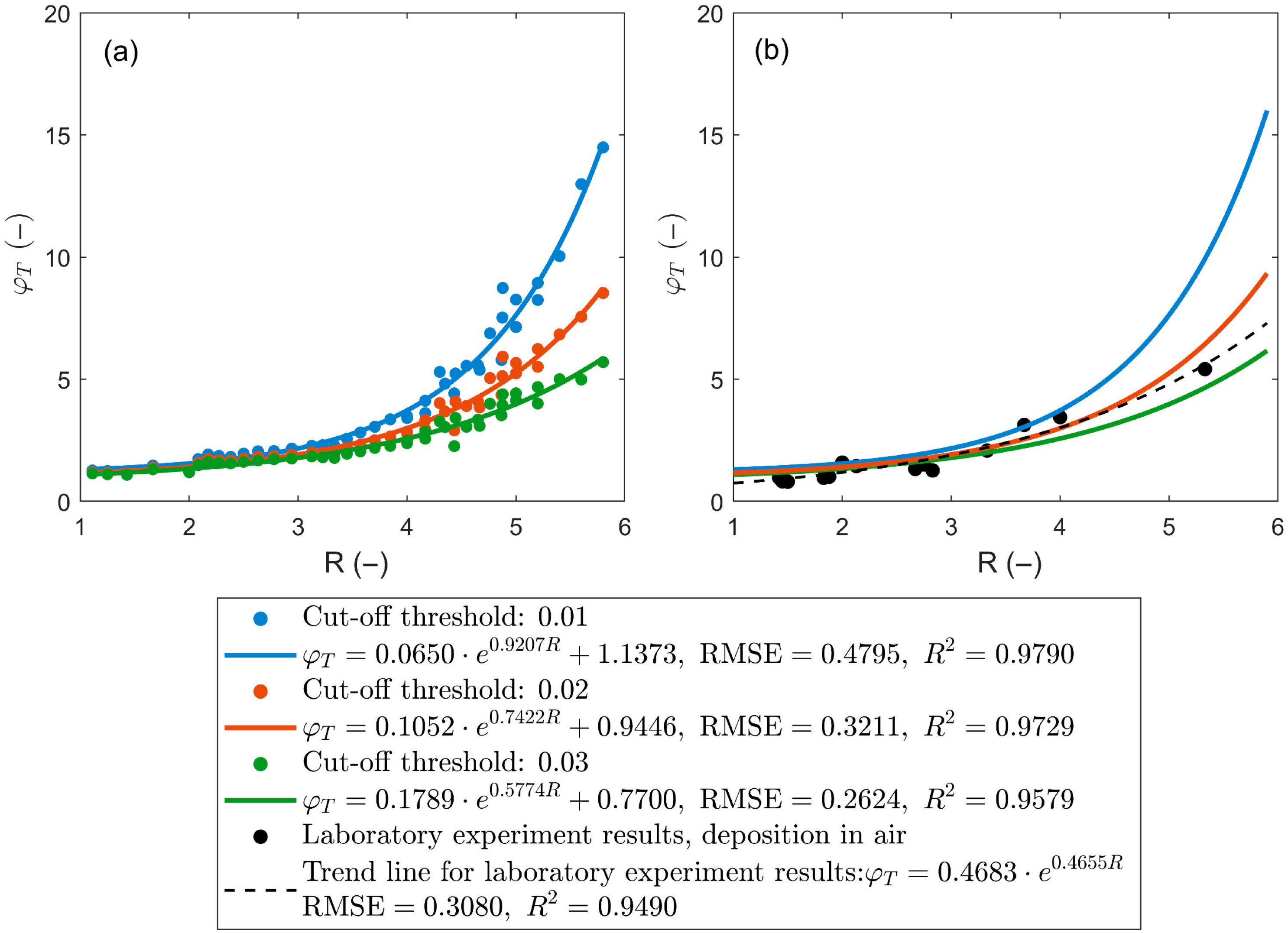
In Figure 15a, computed transition layer lengths are shown using thresholds of 0.01, 0.02, and 0.03 for the numerically generated samples. To minimize the influence of randomness, results from three repeated experiments for each R value are averaged. The error range for transition layer length determined by this new method lies between 0.005 and 0.90, with an average error of 0.16. The φTR trends determined using different density thresholds all follow an exponential distribution. As the density threshold decreases, the artificially defined lower boundary of the transition layer shifts downward, correspondingly increasing the transition layer length.
In Figure 15b, black scatter points and dashed line represent the laboratory results under in-air deposition using the piecewise linear segmentation method and the corresponding φT–R trend line determined. Comparing the four trend lines shows that when 0.02 is used as the density threshold, the results from the improved method align well with those determined by the piecewise linear segmentation method. To ensure comparability across datasets in this study, a uniform density threshold of 0.02 is adopted for analyzing the numerical simulation results with the improved method.
It is worth noting that there is no single “correct” density threshold. When a lower density threshold is selected, subtle influences of the top-layer infiltrating particles on the porosity of the base-layer sediment can be captured. Conversely, a higher density threshold focuses more on regions where the infiltrating particles have a significant impact on the porosity of the base sediment. The threshold value can be defined based on the specific research context.

4.2.3. Empirical Relationship for LTR, nmR and nminR

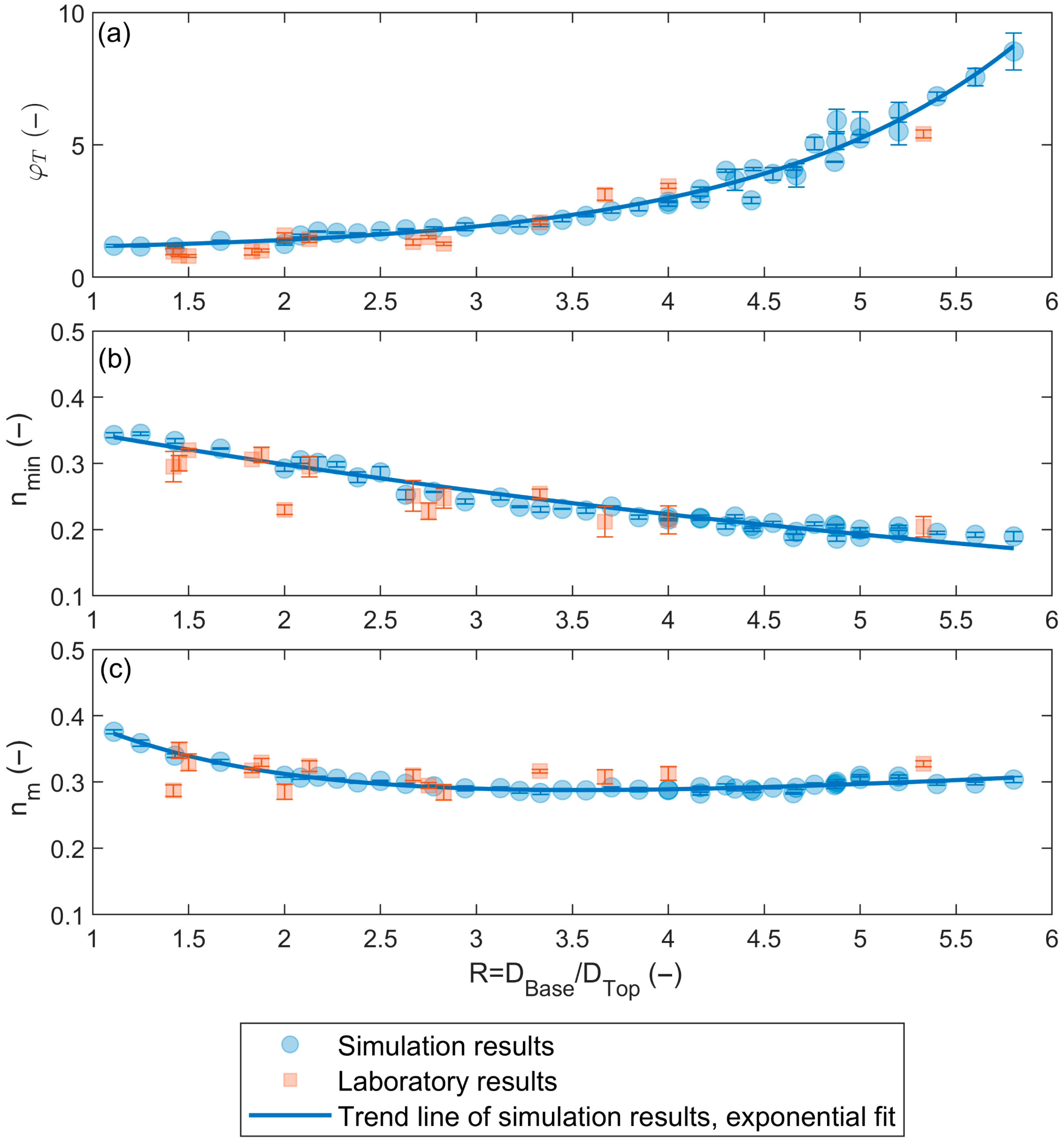
Based on the results presented in the last section, a 2% density threshold was applied throughout to process the simulation data generated during the second stage. This yielded the transition layer length and the average porosity corresponding to each grain-size ratio R. Figure 16 presents the relationships between R and three key parameters: the transition layer length, the minimum porosity, and the average porosity. For comparison, the corresponding laboratory measurement results (introduced in Figure 6 and Figure 7) are also included in the figure.
Transition Layer Length: As illustrated in Figure 16a, the relationship between the dimensionless transition layer length φT and the grain-size ratio R can be well described by an exponential function. Based on three repeated simulations, the average measurement error of φT is 0.16. For glass bead materials, numerical results indicate that when R > 5.8, the fine particles in the top layer achieve nearly unlimited penetration into the underlying coarse matrix. This threshold aligns closely with the critical grain-size ratio R′ = 6.1 reported by [48]. The relationship between φT and R can be described by the following empirical formula:
Glass beads (1 ≤ R ≤ 5.8):
  L T D B a s e = 0.1052 · e 0.7422 · R + 0.9446         ( R M S E = 0.321 ,   R 2 = 0.973 )
Minimum Porosity in the Transition Layer: Figure 16b shows that the minimum porosity nmin within the transition layer decreases with increasing R. At R = 1, nmin is approximately 0.35, which is consistent with the theoretical porosity of a uniform packing (0.36). As R approaches the critical threshold R′, the minimum porosity stabilizes at around 0.19. The average measurement error for nmin is 0.003. The empirical relationship is given by:
Glass beads (1 ≤ R ≤ 5.8):
n m i n = 0.3992 · e 0.1455 · R         ( R M S E = 0.011 ,   R 2 = 0.950 )
Average Porosity in the Transition Layer: As presented in Figure 16c, the average porosity nm within the transition layer initially decreases with increasing R, reaching a minimum around R = 3.5. Beyond this point, the average porosity remains relatively stable at approximately 0.3. The average error in nm measurements is 0.003. The corresponding empirical formula is:
Glass beads (1 ≤ R ≤ 5.8):
n m = 0.3526 · e 0.8938 · R + 0.2296 · e 0.0487 · R       ( R M S E = 0.006 ,   R 2 = 0.923 )
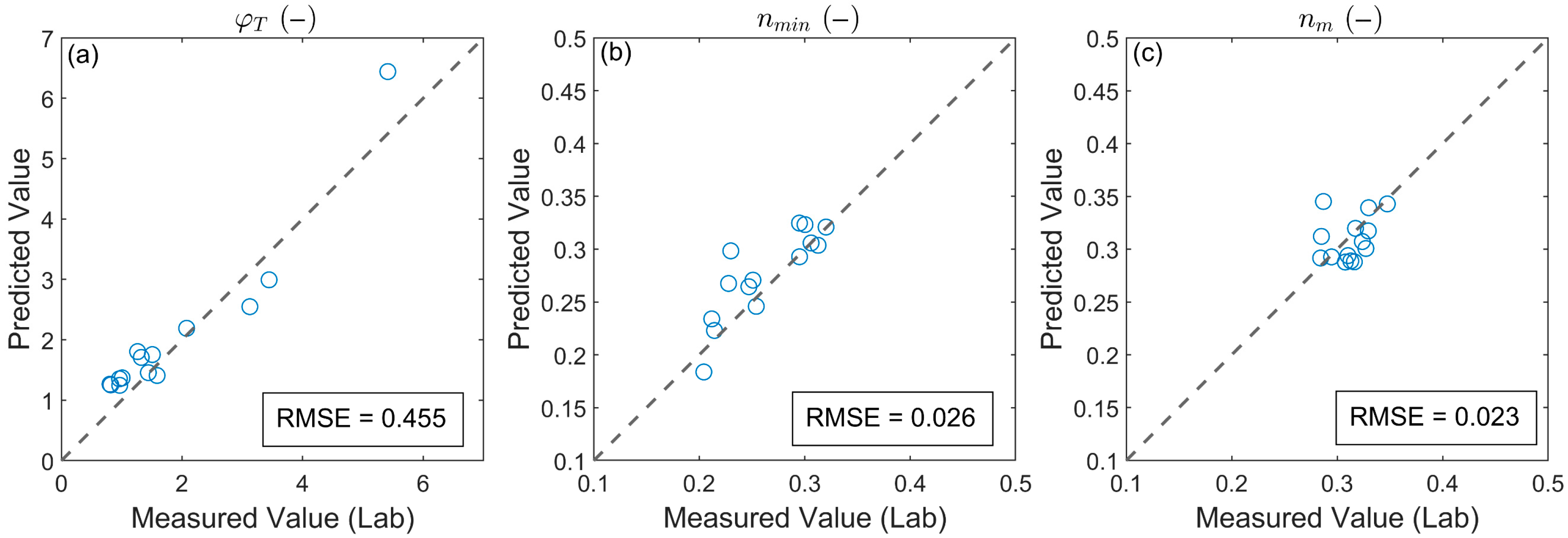
In addition, a comparison between the laboratory measurements and the numerical simulation results in Figure 16 shows that the two datasets are in close agreement. The comparison between the predictions using Equations (19)–(21) and the experimental values (Figure 17) reveals that the average prediction error for the transition layer length is less than half the diameter of the base-layer sediment particles. For both the minimum and average porosity within the transition layer, the average prediction error is only approximately 0.025. These results demonstrate that the empirical formulas derived from the numerical simulations provide accurate and reliable predictions.
Using Equations (19)–(21), we independently verified the accuracy of the model proposed in Section 2. The results show that the simplified porosity model can accurately estimate the average porosity of layered samples. Details are provided in Appendix E. It is worth noting that while the combination of the empirical Equations (19)–(21) and the calculation model (3) allows for the estimation of the average porosity of a stratified sample, it does not provide the volume fractions of each grain-size class within the sample. As a result, it cannot answer the following question: if the sediment in the stratified sample were fully mixed, what would be the porosity of the resulting homogeneous sample? Therefore, to quantitatively evaluate the porosity difference between stratified and uniformly mixed samples with identical sediment composition, further refinement of the calculation model is required.

5. Discussion

5.1. Advantages and Limitations of the Calculation Model

The calculation model proposed in Section 2 is based on a weighted average of the porosities of different sediment layers. Its main advantage lies in its simplicity: the average porosity of a stratified sample can be determined using only the total sample height and the internal grain-size arrangement, without measuring the thickness of each layer—a task difficult to accomplish accurately by visual inspection. This approach thus greatly simplifies field sampling and measurement. Furthermore, the model can be applied to stratified samples formed under flow conditions, since the effects of hydraulic and other depositional factors on transition-layer thickness (LT) and porosity (nm) can be incorporated by correcting the empirical LTR and nmR relationships given in Section 4.2.3, without altering the model structure.
The model, however, has certain limitations. It provides only the overall sample porosity and cannot reflect the minimum porosity within individual transition layers, making it unsuitable for analyzing localized low-permeability zones. Moreover, it assumes that all transition layers are fully developed—an idealization in which each layer consists of only two particle-size classes. In natural settings, a limited upper-layer sediment supply may lead to the premature deposition of finer particles before full transition-layer development. Transition layers containing multiple particle-size fractions, therefore, warrant further study and may require refinement of the present model.

5.2. Analysis of Discrepancies Between Experimental Findings and Existing Literature

To verify the reliability of the transition layer length determined in this study, a comparison with Propster’s results [48] is presented in Section 3.2. This subsection focuses on the deviations observed when R < 1 and R > 4 (Figure 8 and Figure 9).
For R < 1, where the top-layer particles are larger than those in the base layer, Propster’s experiments—though also conducted under dry conditions—involved freely falling large particles that impacted the base layer with significant momentum, resulting in deeper embedding. In contrast, this study placed large particles with zero initial velocity. This difference in deposition methods likely explains the longer transition layer reported by [48]. Clearly, when R < 1, the transition layer length depends not only on particle size ratio but also on the deposition method. Nevertheless, even under high-momentum conditions, Figure 9 shows the embedding depth never exceeded twice the particle diameter, suggesting a limited impact on overall porosity.
For R > 4, this study reports 15% shorter transition layers than [48], likely due to differences in measurement methods. Here, the piecewise linear segmentation method was used, which identifies the transition layer based on noticeable changes in porosity distribution caused by significant infiltration. In contrast, ref. [48] used vertical slicing to visually identify infiltrated particles, allowing even minimal infiltration to be recorded as part of the transition layer. Thus, infiltration depth may be underestimated in this study when small particles are few and do not cause a marked porosity shift.
Although discrepancies exist for R > 4, it is not possible to conclude which method is more accurate, as [48] did not define specific criteria for identifying the boundaries of the transition layer.

5.3. Discussion on the Improved Method for the Transition Zone Identification

The absence of a clear definition for the transition layer range has hindered the comparability of experimental results across studies. The method introduced in Section 4.1.3—based on a density threshold to define the transition layer boundaries—addresses this issue by enabling consistent and objective identification of both the upper and lower limits of the transition layer. This approach significantly improves the comparability of results obtained under different experimental conditions.
While applying a density threshold requires knowledge of the density distribution curves of both the top and base sediments, this information is readily obtainable in numerical simulations. In laboratory experiments, although more challenging, the same data can be acquired using the measurement setup described in Section 3.1.1. The proposed procedure is as follows: Specifically, after forming the base sediment layer, its porosity distribution should be measured immediately to derive its density profile. The fluid is then drained, and the base layer is dried without disturbing its internal structure. The top-layer particles are subsequently deposited to form the stratified sample, and a second porosity measurement is conducted to obtain the total density distribution. The difference between the two curves yields the density profile of the top sediment, from which the transition layer thickness can be calculated using the predefined density threshold.
This procedure demonstrates that the improved method for determining the transition layer range is broadly applicable to both numerical and experimental contexts, providing a more robust framework for comparative sediment studies.

5.4. Discussion on the Limitations of the Laboratory Experiment Method

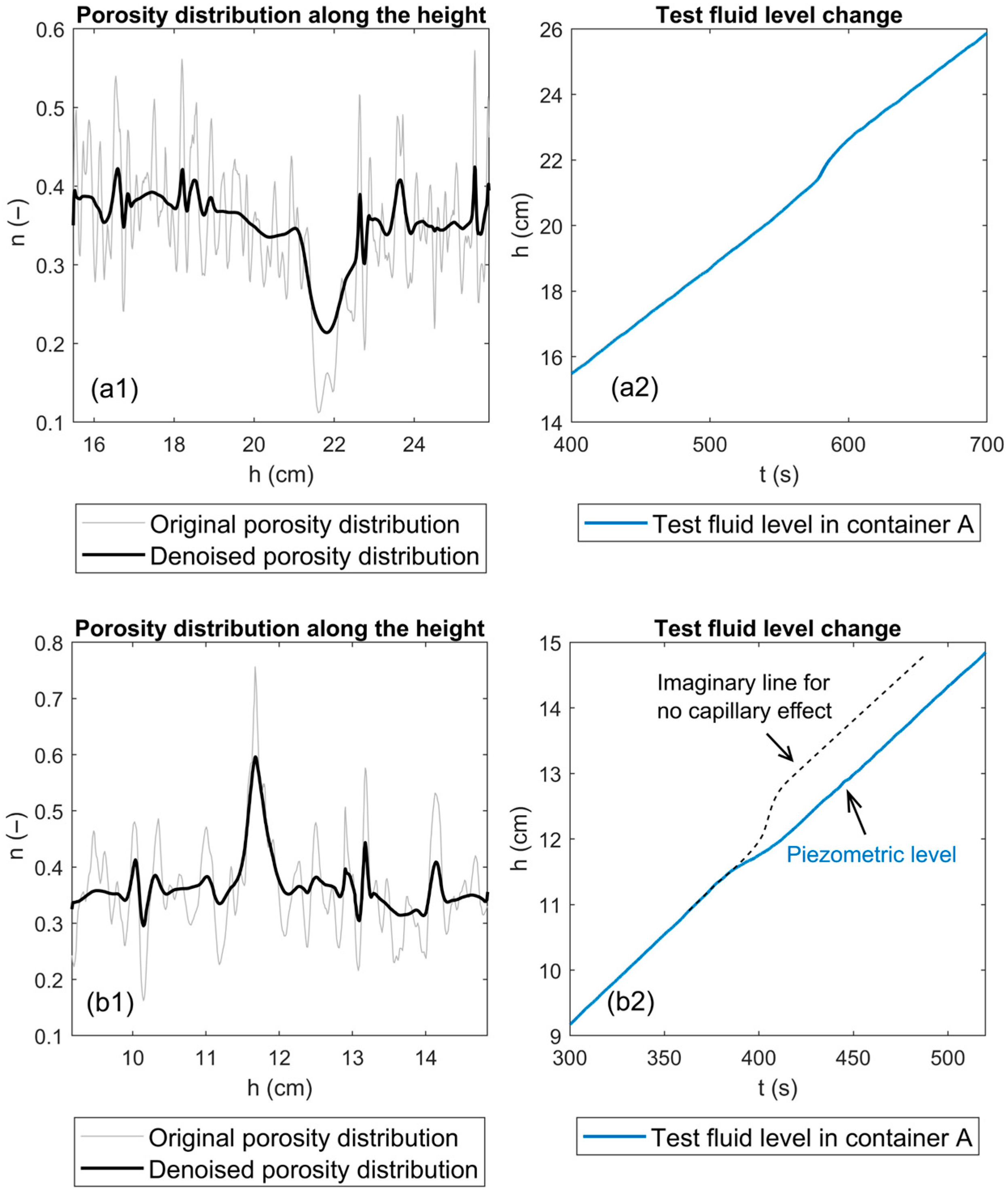
Impact of capillary action: As noted, the smallest particle diameter used in the laboratory experiments was 3 mm. When smaller particles are employed, capillary action significantly affects the test fluid level within the sediment, making the method unsuitable for determining transition layer thickness:
In the experiment shown in Figure 18(a1,a2), the fluid level in the sediment and pressure tube remained nearly identical throughout the measurement, confirming negligible capillary influence. In contrast, for the experiment shown in Figure 18(b1,b2), it was observed that as the measuring fluid approached the finer top layer (1.5 mm particles), the fluid level in the sediment began rising faster than in the pressure tube, stabilizing at a 4 mm difference once the measuring fluid fully entered the top layer (Figure 4). This led to a misinterpretation of the porosity trend in the transition zone: instead of the expected decrease followed by an increase (Figure 18(a1)), an incorrect increase–decrease trend was recorded (Figure 18(b1)). The underlying cause is that capillary action draws some fluid upward without contributing to hydrostatic pressure, effectively reducing the detectable volume change and slowing the apparent rise in pressure (Figure 18(b2)).
Impact of Wall Effect on Experimental Results: As discussed in Section 3.1.1, the use of a cylindrical container with rigid walls introduces a wall effect during sediment formation, leading to increased porosity near the container boundaries. The elevated porosity in this region may facilitate deeper infiltration of the top-layer particles. It is necessary to examine whether this phenomenon significantly affects the accuracy of transitional layer length measurements.
Figure 19 presents laboratory results obtained under dry conditions, grouping experiments with similar R values but differing base layer particle diameters DBase into four categories. Within each group, despite differences in DBase and the associated variation in the wall effect’s spatial extent, no significant differences in measured transitional layer lengths were observed.
These findings suggest that variations in base sediment porosity within the range of 0.36 to 0.4 do not exert a significant influence on the infiltration depth of overlying sediment particles. This result expands the applicability of the infiltration depth analysis, indicating that the conclusions drawn are robust across a range of base sediment porosities rather than being limited to a specific porosity condition.

5.5. Discussion on the Influence of Water on the Transition Layer Length

As shown in Figure 8 and Figure 9, when R is less than 3, the transition layer length of stratified samples formed under in-water deposition conditions is significantly lower than that under in-air deposition conditions. However, when R is greater than 3, no obvious difference is observed between the two conditions. The following discussion focuses on the influence of water on the formation of the transition layer within different R value ranges.
When R is less than 1, as introduced, the formation of the transitional layer results from the interference and embedding of the top-layer large spheres into the base-layer small spheres. The presence of water significantly reduces the embedding depth of the top-layer large spheres. The most direct hypothesis is that buoyancy reduces the mass of the top sediment layer, thereby decreasing the embedding depth. However, in cases where the top-layer spheres are larger than those in the base layer, this study continuously added top-layer particles until no further embedding was observed, indicating that the weight of the top sediment layer was sufficiently large and the embedding depth reached its limit. Therefore, the potential influence of buoyancy can be excluded. Moreover, since the top layer particles were placed onto the base layer sediment under zero initial velocity in both water and in-air conditions, the weakening effect of water on particle falling velocity and momentum can be disregarded in this study. Ishibashi et al. [68], through studying glass beads sliding on a glass surface and comparing dry conditions to fully water-submerged conditions, found that the static friction coefficient increased from ~0.162 (dry) to 0.277 (submerged), indicating that water hinders particle motion within sediment packings. This increase is partly due to hydrogen bonding between water molecules and particle surfaces, which enhances adhesion and friction [69]. Moreover, as pores saturate, any particle rearrangement must displace pore water, introducing viscous resistance. This resistance arises from the fluid’s viscosity and reflects viscous compaction mechanisms common in saturated sediment systems [70,71]. Taken together, under water deposition conditions, the base layer particles can be imagined as being partially fixed by a glue-like effect, weakening the interference and embedding of the top layer large spheres into the base sediment.
When R is greater than 1 but less than 3, although the top-layer particles are smaller than those in the base layer, experimental results show that the sediment infiltration depth is very limited, generally less than twice the diameter of the base-layer spheres (2·DBase). This is considered to be because the pore sizes between the base-layer particles are comparable to or slightly larger than the top-layer particle diameters, thereby restricting sediment infiltration. In this case, when top-layer small spheres enter pores of similar size to their own volume, it is accompanied by the complete expulsion of pore water. The relative movement between the expelled water and the infiltrating particles limits the rapid infiltration of particles. When particle velocity decreases to zero, the water-induced increase in static friction between glass particles further limits continued infiltration, resulting in a reduced transitional layer length.
When R increases further, the pore size between the base layer particles becomes much larger than the infiltrating particle size, and the effect of pore water expulsion on infiltration rapidly diminishes. The infiltration of top-layer particles then mainly depends on the dynamic and static friction coefficients between the glass particles. Compared to the in-air condition, the approximately 70% increase in friction coefficient under water appears to have only a limited effect on reducing sediment infiltration.
This analysis of the influence of water on the transitional layer length shows that when R is greater than 3, the effect of water is weak and can be neglected. This finding is meaningful for numerical simulations because it implies that to save computational cost, the interaction between water and particles can be omitted in simulations when R > 3. However, when R is less than 3, the influence of water increases, and to improve the accuracy of numerical simulations, the interaction between water (especially pore water) and settling particles needs to be considered.
For fluvial sediment, the empirical equations derived under in-air conditions in this paper can slightly overestimate the length of the transitional layer for stratified samples with R < 3. However, when the actual transition layer thickness L is smaller, the mean porosity nm of the transition layer correspondingly increases (because the amount of infiltrating sediment is limited, resulting in only a minor porosity reduction due to grain-size mixing). This implies that the product of L and nm may remain nearly constant, thereby having a limited impact on the porosity of stratified samples as calculated by Equation (3).

5.6. Advantages and Limitations of Numerical Simulations

The use of numerical simulations in this study, specifically via the DEM-based software Particula 1.3, offers several advantages alongside important limitations.
One of the key strengths of simulation with Particula 1.3 is its ability to resolve the internal structure of the sediment at the grain scale. Unlike laboratory measurements, the simulation provides spatial coordinates of each particle in a generated packing, enabling precise determination of porosity and density profiles. This capability supports the improved, density-threshold-based method for identifying transition layers, which enhances consistency and reduces subjectivity in data analysis.
Simulations also allow for controlled, repeatable testing across a broader range of conditions. In this study, they were used to extend the dataset beyond the practical limits of laboratory testing, particularly for high grain-size ratios (R). The resulting empirical relationships for transition layer thickness and porosity values are grounded in a far more diverse parameter space than would be feasible through experiments alone. The empirical relationships derived from the numerical samples (10 cm core) were fitted and validated against laboratory results (20 cm samples), showing satisfactory predictive accuracy.
Despite these advantages, numerical simulations with Particula 1.3 have limitations. Most notably, it is not currently possible to model fluid-particle interactions—such as pore water displacement—using Particula 1.3. This restricts the accuracy of simulations for low grain-size ratios (R < 3), where the influence of water on particle infiltration is shown to be significant. Additionally, the computational cost imposes practical constraints. On a normal computer equipped with an Intel i7/i9 processor and 64 GB of RAM, the maximum number of particles that can be simulated is approximately 65,000 based on our tests. This limits the achievable sample size, particularly when simulating fine particles or large-scale systems.

6. Conclusions and Outlook

As Part I of a two-part study, this paper integrates laboratory experiments and numerical simulations to investigate the development of transition layers and porosity distribution in stratified sediment samples.
The study demonstrates that a distinct transition layer forms between adjacent homogeneous layers, with its structure and extent governed by the grain-size ratio (R) between them. When fine sediments overlie coarser ones, the transition layer develops through particle infiltration, and its thickness increases with R.
Empirical relationships derived from calibrated numerical simulations provide a practical means to estimate both the transition-layer thickness and its average porosity, enabling the prediction of overall porosity in stratified samples based solely on R.
Beyond its methodological contributions, this work underscores that stratification-induced porosity variations can significantly influence permeability, water exchange, and nutrient transport in sedimentary environments. These insights establish a quantitative basis for linking microscopic grain interactions to macroscopic sedimentary behavior.
Although the empirical formulas proposed in this paper enable the estimation of the average porosity of stratified samples, they do not allow for the determination of the volume fractions of different grain-size classes within the sample. As a result, the porosity difference between a stratified sample and a well-mixed sample with the same sediment composition cannot be quantitatively assessed. Therefore, further refinement of the porosity calculation model introduced in this paper is necessary—this forms the core focus of Part II of the present study.

Author Contributions

Conceptualization, W.X.; methodology, W.X.; software, W.X.; validation, W.X.; formal analysis, W.X.; investigation, W.X.; resources, W.X.; data curation, W.X.; writing—original draft preparation, W.X.; writing—review and editing, C.B.; visualization, W.X.; supervision, C.B.; All authors have read and agreed to the published version of the manuscript.

Funding

This study was funded by the German Research Foundation (Deutsche Forschungsgemeinschaft, Grant Number SCHU 1054/6-2).

Institutional Review Board Statement

Not applicable.

Informed Consent Statement

Not applicable.

Data Availability Statement

The original data presented in the study are openly available in Zenodo at https://zenodo.org/records/15680592 (accessed on 22 October 2025).

Acknowledgments

The effort of the crew of the Model construction and the Metrology during the laboratory experiments is appreciated. We deeply thank Mingxuan Bao, Zhen Wei and Yan Chen for their support during the numerical simulations.

Conflicts of Interest

The authors declare no conflicts of interest.

Abbreviations

The following abbreviations are used in this manuscript:
Pthe probability of bridging the pores in the coarse matrix by fine sediment
βtrapping coefficient to compute the fraction of fine sediment trapped in the bed
ffine sediment volume fraction for P- and β-model
f0fine sediment volume fraction at the bed surface P- and β-model.
AA and ABthe cross-sectional areas of containers A and B
ΔhA and ΔhBwater level change in containers A and B
vA and vBthe rates of water level change in containers A and B
DTop and DBasediameter of the top-layer and base-layer spheres
DGraindiameter of spheres in a measurement container
DContainerdiameter of the measurement container
nporosity value measured within a container of finite size
n0porosity value measured in an infinitely large container
nmthe average porosity of the transition layer
nminthe minimum porosity within the transition layer
ntotalporosity value in a slice (1 − ρSolid)
nstratifiedaverage porosity of a stratified structure
nwell-mixedporosity of a well-mixed sediment sample
VSlicevolume of a slice including the volume of top-layer and base-layer particles and the pores.
VBasevolume of the base-layer particles in a slice
VTopvolume of the top-layer particles in a slice
ρBasedensity of the base-layer particles in a slice
ρTopdensity of the top-layer particles in a slice
ρsoliddensity of all particles in a slice (ρBase + ρTop)
ρcut-offdensity threshold to identify the lower boundary of the transition layer
ρ0density of top-layer particles at the base matrix surface
ρ1density of top-layer particles at the penetration beginning line
Rsize ratio between the top-layer and base-layer spheres (DBase/DTop)
Rccritical size ratio between the large and small spheres when percolation of small particles is possible
Rcritical value of R corresponding to the onset of unlimited percolation of top-layer particles
LTransition_layerlength of the transition layer
φdimensionless penetration depth
φTdimensionless transition layer length (LTransition layer/DBase)
φ*Tdimensionless transition layer length (LTransition layer/max(DBase, DTop))
Xvolume fraction of particles with a certain size
v r e l relative velocity at the contact point for two contacting particles
v linear velocity
ω angular velocity
r contact radius vector from the center of mass of a particle to the contact point
J n normal impulse
n contact normal vector, perpendicular to the contact surface at the point of contact
J t tangential impulse
J total impulse J =   J n + J t
m mass of a particle
F e x t external forces
τ e x t external torques
I inertia tensor
x position quaternion
q orientation quaternion

Appendix A

Figure A1. (a) Wall effect influence range under hard boundary conditions. (b) Wall effect influence range under soft boundary conditions.
Geotechnics 05 00077 g0a1

Appendix B

Figure A2. Sensitivity study based on R = 3.33: Comparison of dimensionless transition layer length measurements under different (a) Solver Iteration Count, (b) Sleep Threshold, (c) Fixed Delta Time, and (d) Drop Rate conditions.
Geotechnics 05 00077 g0a2
Solver Iteration Count: to solve the conservation of momentum equations on multiple contacts. The number of iterations required is typically less than 10 to obtain reasonable results [58]. Indeed, the change in Solver Iteration Count from 40 to 60 has little effect on the experimental results.
Sleep Threshold: If a grain’s energy (divided by a reference energy) falls below this threshold, it’s considered at rest and excluded from future solver iterations until reactivated by interaction. This helps reduce computational cost. The results show that even when the Sleep Threshold is further reduced below 0.5·10−3—the value used in this study—the measured thickness of the transition layer remains largely unchanged.
Fixed Delta Time: the simulation advances in uniform time intervals. A smaller delta time increases accuracy and stability, especially in fast or stiff systems, but also increases simulation time. The sensitivity study found that when the time interval exceeds 10·10−3 (s), the numerical simulation becomes unstable, primarily manifested by particles penetrating the soft boundary during settling. In contrast, when the time interval is below 5·10−3 (s), the measured thickness of the transition layer shows no significant variation.
Drop Rate: When the Drop Rate is less than 1.8·10−4 (m3/(m2·s)), the measured thickness of the transition layer shows no significant variation. This confirms that the value of Drop rate used in this study is sufficiently small to ensure that the transition layer thickness is not reduced by an excessively high sediment supply rate.

Appendix C

Table A1. Particle size ratios used in the numerical simulations.
Simulation with Glass Beads
DBase − DTop (mm)RDBase − DTop (mm)R
10 − 91.1112 − 34.00
10 − 81.2510 − 2.44.17
10 − 71.4312.5 − 34.17
10 − 61.6712.9 − 34.30
10 − 52.0010 − 2.34.35
10 − 4.82.0813.3 − 34.43
10 − 4.62.1710 − 2.254.44
10 − 4.42.2710 − 2.24.55
10 − 4.22.3810 − 2.154.65
10 − 42.5014 − 34.67
10 − 3.82.6310 − 2.14.76
10 − 3.62.7814.6 − 34.87
10 − 3.42.9411.7 − 2.44.88
10 − 3.23.1310 − 2.054.88
10 − 3.13.2310 − 2.05.00
10 − 33.3315 − 35.00
10 − 2.93.4511.44 − 2.25.20
10 − 2.83.5715.6 − 35.20
10 − 2.73.7016.2 − 35.40
10 − 2.63.8516.8 − 35.60
10 − 2.54.0017.4 − 35.80

Appendix D

Figure A3. Vertical cross-sections of stratified samples at different y-positions under the condition R = 1.
Geotechnics 05 00077 g0a3

Appendix E

Appendix E.1. Method for Validating the Accuracy of the Calculation Model (3)
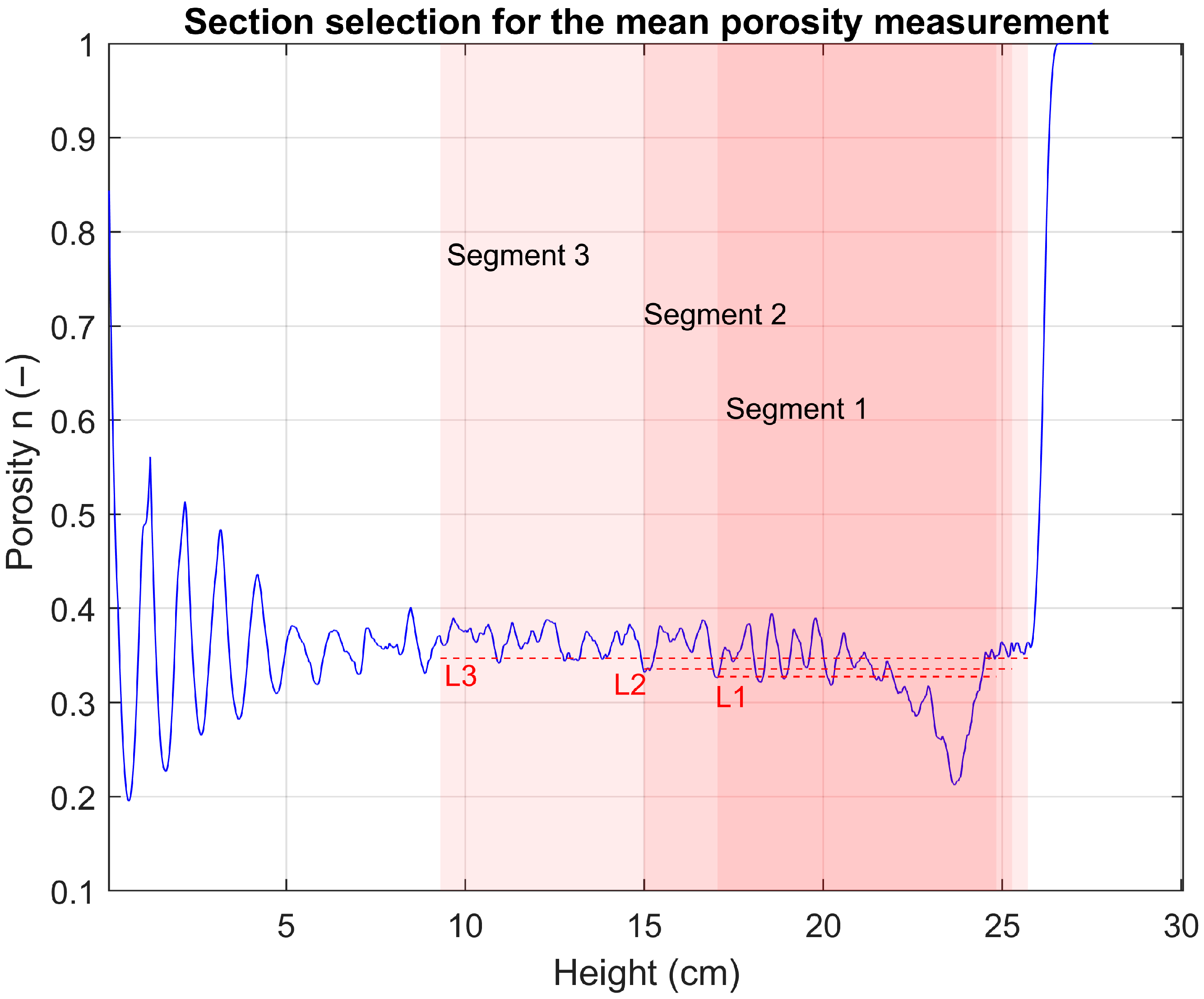
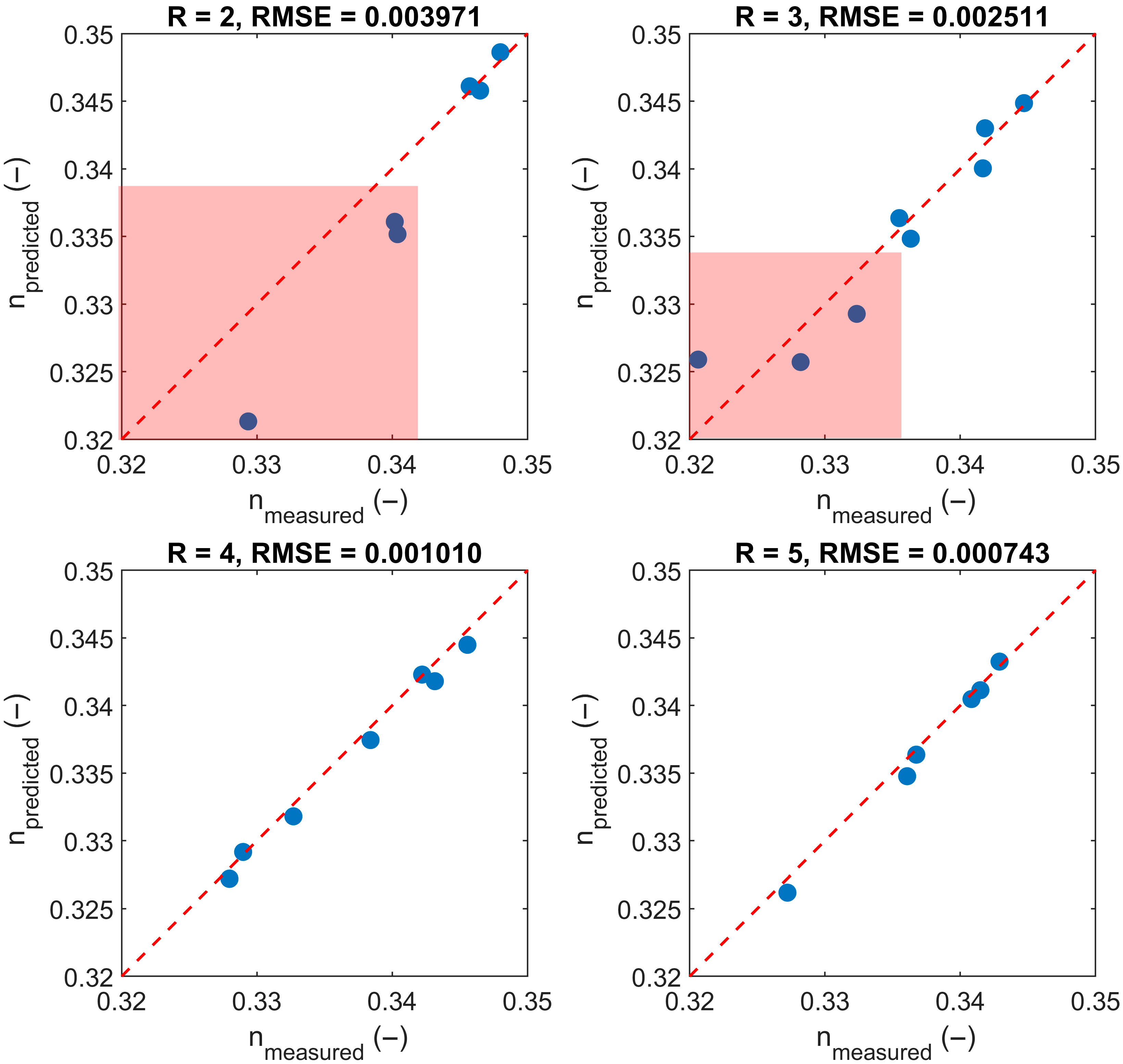
Numerically generated layered samples with R = 2, 3, 4, and 5 were adopted. For each R value, two samples were considered to reduce the influence of randomness.
For each layered sample, we first obtained its porosity profile along the vertical (height) direction (Figure A4). Using MATLAB R2024b, we extracted sub-segments of varying lengths from the same sample; each extracted segment was ensured to clearly include the transition layer. The measured average porosity of a segment, nmeasured, was then computed by averaging the porosity profile over that segment. The total segment length L and the intra-sample particle-size ratio R were also recorded.
Figure A4. Segments selected for the mean porosity measurement.
Geotechnics 05 00077 g0a4
Employing empirical Equations (19) and (21), we calculated the transition-layer thickness and its mean porosity, and used these quantities as known inputs to Calculation Model (3) to obtain the predicted porosity, npredicted. Finally, nmeasured and npredicted were compared across the different R values.

Appendix E.2. Results

The comparison results show that for all tested R combinations, the RMSE between nmeasured and npredicted is below 0.004, and the relative error remains below 2% in all cases. However, when R = 2 or R = 3, noticeably larger discrepancies appear between nmeasured and npredicted, particularly in the regions marked in Figure A5. These cases correspond to sample segments whose total length gradually approaches the thickness of the transition layer. Under such conditions, the lengths of the homogeneous layers in the stratified sample become significantly reduced, amplifying the influence of natural fluctuations in porosity on the measured porosity within that range. Consequently, nmeasured no longer remains stably around 0.36 but exhibits considerable oscillations.
This effect, however, is not accounted for in Model 3, which assumes that the porosity of the homogeneous layers remains constant at 0.36 regardless of their length. When R > 3, the transition layer thickness increases substantially, and its relative influence on the overall sample porosity becomes more pronounced. This, in turn, diminishes the impact of porosity fluctuations within the homogeneous layers, leading to noticeably smaller discrepancies between nmeasured and npredicted.
In summary, the consistently low error between nmeasured and npredicted confirms the applicability of Calculation Model 3.
Figure A5. Comparison between nmeasured and npredicted.
Geotechnics 05 00077 g0a5

References

  1. Pszonka, J.; Schulz, B. SEM Automated Mineralogy applied for the quantification of mineral and textural sorting in submarine sediment gravity flows. Gospod. Surowcami Miner. Miner. Resour. Manag. 2022, 38, 105–131. [Google Scholar] [CrossRef]
  2. Pszonka, J.; Godlewski, P.; Fheed, A.; Dwornik, M.; Schulz, B.; Wendorff, M. Identification and quantification of intergranular volume using SEM automated mineralogy. Mar. Pet. Geol. 2024, 162, 106708. [Google Scholar] [CrossRef]
  3. Chwang, A.T.; Chan, A.T. Interaction Between Porous Media and Wave Motion. Annu. Rev. Fluid Mech. 1998, 30, 53–84. [Google Scholar] [CrossRef]
  4. Ting, C.-L.; Lin, M.-C.; Cheng, C.-Y. Porosity effects on non-breaking surface waves over permeable submerged breakwaters. Coast. Eng. 2004, 50, 213–224. [Google Scholar] [CrossRef]
  5. Frings, R.M.; Kleinhans, M.G.; Vollmer, S. Discriminating between pore-filling load and bed-structure load: A new porosity-based method, exemplified for the river Rhine. Sedimentology 2008, 55, 1571–1593. [Google Scholar] [CrossRef]
  6. Frings, R.M. Sedimentary Characteristics of the Gravel-Sand Transition in the River Rhine. J. Sediment. Res. 2011, 81, 52–63. [Google Scholar] [CrossRef]
  7. Vollmer, S.; Kleinhans, M.G. Predicting incipient motion, including the effect of turbulent pressure fluctuations in the bed. Water Resour. Res. 2007, 43, W05410. [Google Scholar] [CrossRef]
  8. El Kadi Abderrezzak, K.; Die Moran, A.; Tassi, P.; Ata, R.; Hervouet, J.-M. Modelling river bank erosion using a 2D depth-averaged numerical model of flow and non-cohesive, non-uniform sediment transport. Adv. Water Resour. 2016, 93, 75–88. [Google Scholar] [CrossRef]
  9. Miwa, H.; Parker, G. Effects of sand content on initial gravel motion in gravel-bed rivers. Earth Surf. Process. Landf. 2017, 42, 1355–1364. [Google Scholar] [CrossRef]
  10. Mulatu, C.A.; Crosato, A.; Moges, M.M.; Langendoen, E.J.; McClain, M. Morphodynamic Trends of the Ribb River, Ethiopia, Prior to Dam Construction. Geosciences 2018, 8, 255. [Google Scholar] [CrossRef]
  11. Frings, R.M.; Hillebrand, G.; Gehres, N.; Banhold, K.; Schriever, S.; Hoffmann, T. From source to mouth: Basin-scale morphodynamics of the Rhine River. Earth Sci. Rev. 2019, 196, 102830. [Google Scholar] [CrossRef]
  12. van Bui, H.; Bui, M.D.; Rutschmann, P. Advanced Numerical Modeling of Sediment Transport in Gravel-Bed Rivers. Water 2019, 11, 550. [Google Scholar] [CrossRef]
  13. Athy, L.F. Density, Porosity, and Compaction of Sedimentary Rocks. AAPG Bull. 1930, 14, 1–24. [Google Scholar] [CrossRef]
  14. Hatch, C.E.; Fisher, A.T.; Ruehl, C.R.; Stemler, G. Spatial and temporal variations in streambed hydraulic conductivity quantified with time-series thermal methods. J. Hydrol. 2010, 389, 276–288. [Google Scholar] [CrossRef]
  15. Aitken, M.J. An Introduction to Optical Dating: The Dating of Quaternary Sediments by The Use of Photon-Stimulated Luminescence; Oxford Science Publications: Oxford, UK; Oxford University Press: New York, NY, USA, 1998. [Google Scholar]
  16. Goff, J.A.; Kraft, B.J.; Mayer, L.A.; Schock, S.G.; Sommerfield, C.K.; Olson, H.C.; Gulick, S.P.; Nordfjord, S. Seabed characterization on the New Jersey middle and outer shelf: Correlatability and spatial variability of seafloor sediment properties. Mar. Geol. 2004, 209, 147–172. [Google Scholar] [CrossRef]
  17. Vollmer, S.; de los Santos Ramos, F.; Daebel, H.; Kühn, G. Micro scale exchange processes between surface and subsurface water. J. Hydrol. 2002, 269, 3–10. [Google Scholar] [CrossRef]
  18. Noack, M.; Ortlepp, J.; Wieprecht, S. An Approach to Simulate Interstitial Habitat Conditions During the Incubation Phase of Gravel-Spawning Fish. River Res. Apps 2017, 33, 192–201. [Google Scholar] [CrossRef]
  19. Hales, T.C.; McLaughlin, S. A proof of the dodecahedral conjecture. arXiv 1998, arXiv:9811079. [Google Scholar]
  20. Donev, A.; Cisse, I.; Sachs, D.; Variano, E.A.; Stillinger, F.H.; Connelly, R.; Torquato, S.; Chaikin, P.M. Improving the density of jammed disordered packings using ellipsoids. Science 2004, 303, 990–993. [Google Scholar] [CrossRef] [PubMed]
  21. Man, W.; Donev, A.; Stillinger, F.H.; Sullivan, M.T.; Russel, W.B.; Heeger, D.; Inati, S.; Torquato, S.; Chaikin, P.M. Experiments on random packings of ellipsoids. Phys. Rev. Lett. 2005, 94, 198001. [Google Scholar] [CrossRef]
  22. Bernal, J.D.; Finney, J.L. Random close-packed hard-sphere model. II. Geometry of random packing of hard spheres. Discuss. Faraday Soc. 1967, 43, 62–69. [Google Scholar] [CrossRef]
  23. Haughey, D.P.; Beveridge, G.S.G. Structural properties of packed beds—A review. Can. J. Chem. Eng. 1969, 47, 130–140. [Google Scholar] [CrossRef]
  24. Carling, P.A.; Reader, N.A. Structure, composition and bulk properties of upland stream gravels. Earth Surf. Process. Landf. 1982, 7, 349–365. [Google Scholar] [CrossRef]
  25. Wu, W.; Wang, S.S.Y. Formulas for Sediment Porosity and Settling Velocity. J. Hydraul. Eng. 2006, 132, 858–862. [Google Scholar] [CrossRef]
  26. Wooster, J.K.; Dusterhoff, S.R.; Cui, Y.; Sklar, L.S.; Dietrich, W.E.; Malko, M. Sediment supply and relative size distribution effects on fine sediment infiltration into immobile gravels. Water Resour. Res. 2008, 44, W03424. [Google Scholar] [CrossRef]
  27. Frings, R.M.; Schüttrumpf, H.; Vollmer, S. Verification of porosity predictors for fluvial sand-gravel deposits. Water Resour. Res. 2011, 47, W07525. [Google Scholar] [CrossRef]
  28. Stovall, T.; de Larrard, F.; Buil, M. Linear packing density model of grain mixtures. Powder Technol. 1986, 48, 1–12. [Google Scholar] [CrossRef]
  29. Ouchiyama, N.; Tanaka, T. Porosity estimation for random packings of spherical particles. Ind. Eng. Chem. Fund. 1984, 23, 490–493. [Google Scholar] [CrossRef]
  30. Yu, A.B.; Standish, N. Estimation of the porosity of particle mixtures by a linear-mixture packing model. Ind. Eng. Chem. Res. 1991, 30, 1372–1385. [Google Scholar] [CrossRef]
  31. Yu, A.B.; Standish, N. Limitation of proposed mathematical models for the porosity estimation of nonspherical particle mixtures. Ind. Eng. Chem. Res. 1993, 32, 2179–2182. [Google Scholar] [CrossRef]
  32. Preclik, T.; Rüde, U. Ultrascale simulations of non-smooth granular dynamics. Comp. Part. Mech. 2015, 2, 173–196. [Google Scholar] [CrossRef]
  33. Schruff, T.; Liang, R.; Rüde, U.; Schüttrumpf, H.; Frings, R.M. Generation of dense granular deposits for porosity analysis: Assessment and application of large-scale non-smooth granular dynamics. Comp. Part. Mech. 2018, 5, 59–70. [Google Scholar] [CrossRef]
  34. Rettinger, C.; Rüde, U.; Vollmer, S.; Frings, R.M. Effect of sediment form and form distribution on porosity: A simulation study based on the discrete element method. Granul. Matter 2022, 24, 118. [Google Scholar] [CrossRef]
  35. Boggs, S. Principles of Sedimentology and Stratigraphy, 4th ed.; Pearson Prentice Hall: Upper Saddle River, NJ, USA, 2012. [Google Scholar]
  36. Mckee, E.D.; Weir, G.W. Terminology for Stratification and Cross-Stratification in Sedimentary Rocks. Geol. Soc. Am. Bull. 1953, 64, 381. [Google Scholar] [CrossRef]
  37. Miall, A.D. The Geology of Fluvial Deposits: Sedimentary Facies, Basin Analysis, and Petroleum Geology, 4th corrected printing; Springer: Berlin/Heidelberg, Germany, 2006. [Google Scholar]
  38. Nichols, G. Sedimentology and Stratigraphy, 2nd ed.; Wiley-Blackwell: Chichester, UK; Hoboken, NJ, USA, 2009. [Google Scholar]
  39. Benito, G.; Sánchez-Moya, Y.; Sopeña, A. Sedimentology of high-stage flood deposits of the Tagus River, Central Spain. Sediment. Geol. 2003, 157, 107–132. [Google Scholar] [CrossRef]
  40. Guccione, M.J. Grain-Size Distribution of Overbank Sediment and Its Use to Locate Channel Positions. In Alluvial Sedimentation; Marzo, M., Puigdefábregas, C., Eds.; Wiley: Hoboken, NJ, USA, 1993; pp. 185–194. [Google Scholar]
  41. Burns, C.E.; Mountney, N.P.; Hodgson, D.M.; Colombera, L. Anatomy and dimensions of fluvial crevasse-splay deposits: Examples from the Cretaceous Castlegate Sandstone and Neslen Formation, Utah, USA. Sediment. Geol. 2017, 351, 21–35. [Google Scholar] [CrossRef]
  42. Chamberlin, E.P.; Hajek, E.A. Fine-sediment Supply Can Control Fluvial Deposit Architecture: An Example From the Blackhawk Formation-Castlegate Sandstone Transition, Upper Cretaceous, Utah, USA. Sediment. Rec. 2022, 20, 1–10. [Google Scholar] [CrossRef]
  43. Li, P.; Hu, K.; Yu, J. Experimental Investigation on the Permeability and Fine Particle Migration of Debris-Flow Deposits with Discontinuous Gradation: Implications for the Sustainable Development of Debris-Flow Fans in Jiangjia Ravine, China. Sustainability 2024, 16, 10066. [Google Scholar] [CrossRef]
  44. Church, M.; Jakob, M. What Is a Debris Flood? Water Resour. Res. 2020, 56, e2020WR027144. [Google Scholar] [CrossRef]
  45. Asbury, H.; Sallenger, J.R. Inverse Grading and Hydraulic Equivalence in Grain-Flow Deposits. J. Sediment. Res. 1979, 49, 553–562. [Google Scholar] [CrossRef]
  46. Todd, S.P. Stream-driven, high-density gravelly traction carpets: Possible deposits in the Trabeg Conglomerate Formation, SW Ireland and some theoretical considerations of their origin. Sedimentology 1989, 36, 513–530. [Google Scholar] [CrossRef]
  47. Tucker, M.E. Sedimentary Rocks in the Field, 3rd ed.; John Wiley & Sons: Hoboken, NJ, USA, 2003. [Google Scholar]
  48. Propster, M.; Szekely, J. The porosity of systems consisting of layers of different particles. Powder Technol. 1977, 17, 123–138. [Google Scholar] [CrossRef]
  49. Sakthivadivel, R.; Einstein, H.A. Clogging of Porous Column of Spheres by Sediment. J. Hydr. Div. 1970, 96, 461–472. [Google Scholar] [CrossRef]
  50. Cui, Y.; Wooster, J.K.; Baker, P.F.; Dusterhoff, S.R.; Sklar, L.S.; Dietrich, W.E. Theory of Fine Sediment Infiltration into Immobile Gravel Bed. J. Hydraul. Eng. 2008, 134, 1421–1429. [Google Scholar] [CrossRef]
  51. Schruff, T. Taking a Closer Look at the Causes and Impacts of Fine Sediment Infiltration into Gravel Beds. Ph.D. Thesis, RWTH Aachen University, Aachen, Germany, 2018. [Google Scholar]
  52. Huston, D.L.; Fox, J.F. Clogging of Fine Sediment within Gravel Substrates: Dimensional Analysis and Macroanalysis of Experiments in Hydraulic Flumes. J. Hydraul. Eng. 2015, 141, 04015015. [Google Scholar] [CrossRef]
  53. Dermisis, D.; Papanicolaou, A.N.T. The effects of protruding rock boulders in regulating sediment intrusion within the hyporheic zone of mountain streams. J. Mt. Sci. 2014, 11, 1466–1477. [Google Scholar] [CrossRef]
  54. Gibson, S.; Heath, R.; Abraham, D.; Schoellhamer, D. Visualization and analysis of temporal trends of sand infiltration into a gravel bed. Water Resour. Res. 2011, 47, W12601. [Google Scholar] [CrossRef]
  55. Wang, L.; Zhang, Y. Interpreting correlations in stress-dependent permeability, porosity, and compressibility of rocks: A viewpoint from finite strain theory. Numer. Anal. Methods Geomech. 2024, 48, 2000–2019. [Google Scholar] [CrossRef]
  56. Zhu, X.; Si, G.; Zhang, C.; Moon, J.-S.; Oh, J. Numerical analysis of hydro-mechanical coupling behaviour during shearing of rock fractures based on an improved friction factor model. J. Rock Mech. Geotech. Eng. 2025, 17, 6079–6094. [Google Scholar] [CrossRef]
  57. Killick, R.; Fearnhead, P.; Eckley, I.A. Optimal Detection of Changepoints with a Linear Computational Cost. J. Am. Stat. Assoc. 2012, 107, 1590–1598. [Google Scholar] [CrossRef]
  58. Al Ibrahim, M.A.; Kerimov, A.; Mukerji, T.; Mavko, G. Particula: A simulator tool for computational rock physics of granular media. Geophysics 2019, 84, F85–F95. [Google Scholar] [CrossRef]
  59. Cundall, P.A.; Strack, O.D.L. A discrete numerical model for granular assemblies. Géotechnique 1979, 29, 47–65. [Google Scholar] [CrossRef]
  60. Pöschel, T.; Schwager, T. Computational Granular Dynamics: Models and Algorithms; Springer: Berlin/Heidelberg, Germany; New York, NY, USA, 2005. [Google Scholar]
  61. Terdiman, P. Memory-Optimized Bounding-Volume Hierarchies. 2001. Available online: https://www.codercorner.com/Opcode.pdf (accessed on 23 April 2025).
  62. Hahn, J.K. Realistic animation of rigid bodies. Comput. Graph. 1988, 22, 299–308. [Google Scholar] [CrossRef]
  63. Mirtich, B.V. Impulsebased Dynamic Simulation of Rigid Body Systems. Ph.D. Thesis, University of California at Berkeley, Berkeley, CA, USA, 1996. [Google Scholar]
  64. Anitescu, M.; Potra, F.A. Formulating Dynamic Multi-Rigid-Body Contact Problems with Friction as Solvable Linear Complementarity Problems. Nonlinear Dyn. 1997, 14, 231–247. [Google Scholar] [CrossRef]
  65. Tonge, R.; Benevolenski, F.; Voroshilov, A. Mass splitting for jitter-free parallel rigid body simulation. ACM Trans. Graph. 2012, 31, 105. [Google Scholar] [CrossRef]
  66. Gavrea, B.I.; Anitescu, M.; Potra, F.A. Convergence of a Class of Semi-Implicit Time-Stepping Schemes for Nonsmooth Rigid Multibody Dynamics. SIAM J. Optim. 2008, 19, 969–1001. [Google Scholar] [CrossRef]
  67. Tang, H.; Song, R.; Dong, Y.; Song, X. Measurement of Restitution and Friction Coefficients for Granular Particles and Discrete Element Simulation for the Tests of Glass Beads. Materials 2019, 12, 3170. [Google Scholar] [CrossRef] [PubMed]
  68. Ishibashi, I.; Perry, C.; Agarwal, T.K. Experimental Determinations of Contact Friction for Spherical Glass Particles. Soils Found. 1994, 34, 79–84. [Google Scholar] [CrossRef]
  69. Peng, L.; Hsia, F.-C.; Woutersen, S.; Bonn, M.; Weber, B.; Bonn, D. Nonmonotonic Friction due to Water Capillary Adhesion and Hydrogen Bonding at Multiasperity Interfaces. Phys. Rev. Lett. 2022, 129, 256101. [Google Scholar] [CrossRef]
  70. Shen, X.; Lin, M.; Pan, F.; Maa, J.P.-Y.; Ha, H.K.; Bi, Q.; Shao, Y.; Zhang, J.; Wu, Z. Viscosity of Cohesive Sediment-Laden Flows: Experimental and Empirical Methods. JGR Oceans 2024, 129, e2023JC020043. [Google Scholar] [CrossRef]
  71. van Elderen, P.; Erkens, G.; Zwanenburg, C.; Middelkoop, H.; Stouthamer, E. Viscous compression of clay and peat. Earth-Sci. Rev. 2025, 260, 104993. [Google Scholar] [CrossRef]
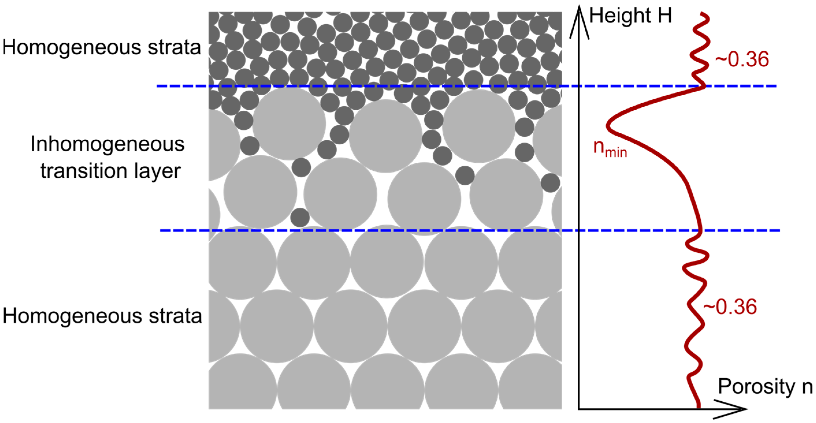
Figure 1. Sketch of a stratified sediment packing and the corresponding qualitative porosity distribution according to [48].
Geotechnics 05 00077 g001
Figure 2. Simplified model for calculating the porosity of a stratified sample.
Geotechnics 05 00077 g002
Figure 3. (a,b) Porosity measurement setup; (c) Pressure sensor and ultrasonic probe; (d) Principle of porosity measurement: The volume corresponding to the product of the cross-sectional area of container A and ΔhA includes both the volume of the sample particles and the pore volume between them. The volume of the test fluid required to fill these pores corresponds to the decrease in fluid volume in container B.
Geotechnics 05 00077 g003
Figure 4. (a) The rising test fluid level in the sample (uniform glass beads 3 mm) is level with that in the pressure tube; (b) Due to the effect of capillarity, the rising test fluid level in the sample (uniform glass beads 1.5 mm) is higher than that in the pressure tube.
Geotechnics 05 00077 g004
Figure 5. (a) Glass beads used in the experiment, with particle sizes from left to right: 20 mm, 16 mm, 11 mm, 8.5 mm, 6 mm, 4 mm, and 3 mm; (bd) Examples of stratified samples—(b) base layer: 8.5 mm, top layer: 11 mm; (c) base layer: 8.5 mm, top layer: 4 mm; (d) base layer: 16 mm, top layer: 4 mm.
Geotechnics 05 00077 g005
Figure 6. (a,b) Smoothed curves of the rising fluid level in container A and the falling fluid level in container B; (c) Determination of the fluid level change rate by calculating the slope of the fluid level–time curve; (d) Porosity distribution calculated based on the rate of fluid level change in containers A and B; (e) Determination of transition layer thickness using the piecewise linear segmentation method, with results shown for two different threshold values; (f) Piecewise linear segmentation of the fluid level–time relationship in container A.
Geotechnics 05 00077 g006
Figure 7. (a) The extent of the transition layer was determined in order to calculate its average porosity, nm. (b) Fourier fit for the rising and falling fluid levels within a fixed window. The point of maximum rise velocity of the fluid surface was identified, and the corresponding porosity value nmin at that location was calculated.
Geotechnics 05 00077 g007
Figure 8. Relationship between the measured dimensionless transition layer length φT and R for stratified samples prepared under in-air and in water deposition conditions. The dimensionless transition layer length φT is defined as the ratio of the transition layer length to the base-layer particle diameter. The dashed line in the figure is plotted based on [48].
Geotechnics 05 00077 g008
Figure 9. Relationship between the measured dimensionless transition layer length φ*T and R for stratified samples prepared under in-air and in water deposition conditions. The dimensionless transition layer length φ*T is defined as the ratio of the transition layer length to the larger of the top- and base-layer particle diameters. The dashed line in the figure is plotted based on [48].
Geotechnics 05 00077 g009
Figure 10. Comparison between the measured porosity of uniform samples at different DGrain/DContainer ratios in this study and the results reported by Frings [27] (the solid line and white diamonds in the figure).
Geotechnics 05 00077 g010
Figure 11. Examples of stratified samples generated by numerical simulation: (a) base layer 12 mm, top layer 3 mm; (b) base layer 15 mm, top layer 3 mm.
Geotechnics 05 00077 g011
Figure 12. Comparison between hard boundary (a) and soft boundary (b).
Geotechnics 05 00077 g012
Figure 13. (a) Slicing of a sample and calculation of the volumes of top-layer particles, base-layer particles, and all particles within each slice. (b) Calculation of the total porosity distribution of the sample and the vertical distribution of top-layer particle density. (c,d) Schematic illustration of the transition layer boundary determined based on the distribution of top-layer particle density. (e) Exponential fitting of the top-layer particle density distribution between the base matrix surface and the penetration begin. (f) Exponential fitting of the top-layer particle density distribution below the penetration begins.
Geotechnics 05 00077 g013
Figure 14. (a,b) Comparison of transition layer length measurements of stratified samples from laboratory experiments and numerical simulations (generated under the same conditions). The dashed line in the figure (a) is plotted based on [48].
Geotechnics 05 00077 g014
Figure 15. (a) Transition layer length measurements obtained using the improved method based on density thresholds of 0.01, 0.02, and 0.03. (b) Comparison of transition layer lengths obtained using the improved method and the linear segmentation method.
Geotechnics 05 00077 g015
Figure 16. (a) Relationship between dimensionless transition layer length φT and R for stratified samples numerically generated using glass beads. (b) Relationship between minimum porosity within the transition layer nmin and R and (c) Relationship between the average porosity of the transition layer nm and R. Data measured in laboratory experiments are plotted for comparison.
Geotechnics 05 00077 g016
Figure 17. (a) Comparison between the predicted dimensionless transition layer length φT using empirical formula and the measured values from laboratory experiments. (b) Comparison between the predicted minimum porosity within the transition layer nmin and the measured values. (c) Comparison between the predicted average porosity of the transition layer nm and the measured values.
Geotechnics 05 00077 g017
Figure 18. (a1,a2) Porosity distribution measured and rising fluid level versus time in container A without capillary effects (base-layer particle diameter 11 mm, top-layer particle diameter 3 mm). (b1,b2) Porosity distribution measured and rising fluid level versus time in container A with capillary effects (base-layer particle diameter 6 mm, top-layer particle diameter 1.5 mm).
Geotechnics 05 00077 g018
Figure 19. Four groups of stratified samples with similar R values but different base-layer particle sizes. The dashed line in the figure is plotted based on [48].
Geotechnics 05 00077 g019
Table 1. The combinations of DBase and DTop.
Deposition in AirDeposition in Water
DBase (mm)DTop (mm)R = DBase/DTopDBase (mm)DTop (mm)R = DBase/DTop
2063.332063.33
1611/8.5/6/4/31.45/1.88/2.67/4.00/5.33164/34.00/5.33
116/4/31.83/2.75/3.67116/31.83/3.67
8.56/4/31.42/2.13/2.838.532.83
64/31.50/2.00632.00
8.5200.438.5200.43
4160.256200.25
3160.19
Table 2. Simulation parameters.
Simulation ParametersModel Calibration and ValidationData Extension
Buffer length fraction (−)00.1
Fixed Delta Time (s)0.005
Solver Iteration Count (−)60
Sleep Threshold (−)0.0005
Shaking Fraction (−)0.001
Bounciness (−)0.926 [67]
Friction coefficient (−)0.16 [67]
Drop rate (m3/(m2·s))1.8·10−4
Density (kg/m3)2500
MaterialsGlass beads
Disclaimer/Publisher’s Note: The statements, opinions and data contained in all publications are solely those of the individual author(s) and contributor(s) and not of MDPI and/or the editor(s). MDPI and/or the editor(s) disclaim responsibility for any injury to people or property resulting from any ideas, methods, instructions or products referred to in the content.