Abstract
Water demand scenarios are defined assuming that the samples are complete. On the other hand, consumption measurements are often affected by a considerable number of missing data. This paper explores the problem of missing data and proposes an example of a data pre-processing technique. Afterwards, a deconstruction of the time series, without being influenced by the presence of gaps, is presented. For this purpose, the fast Fourier transform for nonuniform sampling is developed. This analysis allows us to generate ergodic and stationary samples, useful for pursuing the generation of water demand scenarios. An application is provided on a water consumption time series recorded in a suburban area of Naples, Italy.
1. Introduction
The water demand scenarios are indispensable and condition us to perform the procedures of design, calibration, and management of a water distribution network. Nevertheless, in the last two decades, several methodologies for water demand modelling have been proposed [1,2,3,4,5,6,7], while the methodologies suggested for the generation of water demand scenarios are still few [8,9].
The generation of water demand scenarios requires the presence of simultaneous measurements of consumption of several users to define the covariance matrix. However, the consumption measurements show missing data, due to transmission errors or the absence of users. The presence of an excessive number of missing data within the single time series nullifies the possibility of evaluating the covariance matrix.
The covariance matrix between users’ consumption must refer to the actual sociological conditions to generate reliable scenarios [10]. Nevertheless, sociological conditions have a rapid variability, so it is useless to try to solve the lack of contemporary data problem by extending the sampling period.
The covariance matrix can be reconstructed, even when the data from which the matrix is computed is asynchronous or incomplete. To obtain a reliable result with this technique, it is necessary to have few non-extended gaps. It is, therefore, necessary to implement a structural analysis methodology of the single time series, accounting for the presence of numerous and extensive gaps.
The authors propose a pre-processing methodology for raw consumption data and a subsequent structural analysis procedure applied to an incomplete time series.
In this work, the case study of Soccavo DMA (Naples, Italy) is analysed; seven years of users’ hourly consumption measures are considered. To carry out the characterization of the gaps, it was essential to have recorded the water consumptions during the bimestrial lockdown that occurred in Italy, due to the epidemic emergency of COVID-19. In fact, the water consumptions recorded during this period referred to a time window in which households were forced to remain permanently inside their homes, eliminating the sociologic component from the potential causes of gaps.
2. Methods and Models
2.1. Pre-Processing of the Dataset
The information content that can be provided by a monitoring system varies according to the time frequency of the recordings of measurements. The most complete data is certainly the impulsive water consumption that occurs at the scale of the single fixture. However, it is not possible to use such information because two problems linked to the high scanning frequency arise. In fact, the high scanning of the measurements can somehow conflict with the privacy of the inhabitants and, furthermore, requires a high computational burden. For these reasons, water companies are not willing to record the water consumption of the individual fixtures at such high frequencies, choosing hourly user data gathering. This data is still able to provide an accurate user characterization. The single hourly measurement of a user defines its relationship with other network users, ensuring the estimate of the covariance matrix.
An hourly measurement, even if zero, is valid information for estimating the covariance matrix. On the other hand, an entire day of absence of measurements does not provide any information contribution. The information content of a time series can, therefore, be derived only from the day that recorded, not only null measurements.
The days of complete absence of measurements may be due to different reasons. Some gaps are random and short, usually due to sensor malfunction, deficiencies in records storage, and transmission, or other recovery procedures issues. These shortages differ from those, due to the prolonged absence of residents inside their homes.
Whatever the reason for the lack of information, it is necessary to define the random or deterministic character of the gap and its extent. In fact, the way of conducting a structural analysis of the time series changes according to the characteristics of the gaps. However, some time series have unacceptably low and discontinuous information content. Under these assumptions, it is necessary to verify whether the measured time series of the single flow meter maintains the ability to provide reliable information for the characterization of the users. To this end, the quality of the series must be assessed.
A proposal to evaluate the qualities of the measurements was presented by Padulano et al. [11], but this analysis does not allow us to characterize the samples according to their gaps. However, a qualitative analysis of the time series cannot ignore the characteristic of the gaps and their influence on the correct reproduction of the sample. The authors, therefore, argue that the procedure proposed by Padulano et al. is valid for the quantification of valid measurements in the sample, but it can be improved with information relating to the randomness of the missing data.
The most widespread method for verifying the randomness characteristic of a time series is the Wald–Wolfowitz runs test [12], a non-parametric statistical test that identifies the homogeneous series through the verification of the randomness of the time series. To identify and characterize the gaps, a runs test is performed on binary data, distinguishing only the missing daily data from the others. This test also allows us to identify the confidence interval relating to the extension of the dataset recorded.
However, as demonstrated in the application of the case study, this approach is helpful for the classification of gaps, but it is not sufficient for carrying out an unsupervised analysis of the gaps. The automatic characterization of a sample from its missing data is possible only with a deep learning process that identifies systematic absences with precise periodicities and recurrences.
Finally, the data pre-processing phase provides the elimination of the outliers [13] and any water losses inside the plumbing. At the end of the preprocessing, the time series can be used for user characterization.
2.2. Structural Analysis of the Time Series
Good quality time series guarantee an adequate knowledge of the consumption of their users. However, to characterize the sample, the time series must have an extension that rarely allows stationarity and ergodicity, due to the rapid variation of the sociological characteristics of users. Neglecting such aspect leads to incorrect information that does not allow us to obtain reliable water consumption predictions. However, the daily consumption has a marked variability around its average value; therefore, it is not recommended to fill the series by inserting information obtained artificially, as this could alter the characterization of the sample.
A possible method to synthetically obtain ergodic and stationary series is to analyse single users’ consumptions for short and stationary periods. At this point, it is worth remembering that the time series may be affected by the presence of missing measurements that cannot be roughly eliminated.
The gaps filling is pursued by different methods ranging from the classic use of the fast Fourier transform (FFT) [14,15] to the use of the artificial neural network [16]. Nevertheless, the hourly consumption has a marked variability around its average value; therefore, it is not recommended to fill the missing data by inserting information obtained artificially, as this could alter the characterization of the sample.
A reconstruction of the periodic and stochastic characteristics of a time series of water consumption is proposed by Arandia et al. [17]. However, the classic formulation of the Fourier transform is defined for constant sampling intervals, whereas the presence of missing data determines a sampling interval of non-uniform records. For this reason, it is necessary to apply a technique suitable for non-uniform data [18,19]. By pursuing this analysis, a certain number of harmonics is obtained for the signal analysed, and it is necessary to select only the significant harmonics, following one of the numerous approaches proposed in the literature [17,20,21,22]. The significant harmonics are used to develop a periodic model using the inverse Fourier transform (IFT), which reconstructs the only periodic deterministic component of the time series analysed.
2.3. Stochastic Analysis of the Residuals
The residuals obtained by subtracting the periodic model from the original demand data are tested by an autocorrelation analysis to determine whether they constitute a random sequence. If the time series presents a residual autocorrelation, it is necessary to use an autoregressive model to eliminate the autocorrelation. There are many proposals for autoregression that supply various levels of analytical interpretation, passing from the simplest AR model to the more articulated ARMA and ARIMA models [17,23,24,25]. After this treatment, the only residues deriving from the autoregressive model would represent the stochastic component of the measured water consumption.
On this stochastic component, a fitting is performed to find the most suitable probability distribution for the specific sample.
3. Application
The rare heritage of the measurements provided by the water company “ABC Napoli”, containing the measurements collected in the Soccavo DMA (Figure 1), located in the north-western area of the city of Naples (Italy), is extremely useful to show the application of the proposed methodology.
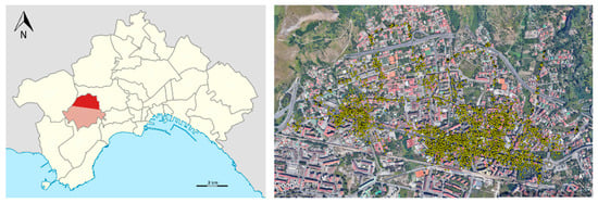
Figure 1.
Soccavo DMA (Naples, Italy), with his flow meters positioned on the map of the area.
In this DMA, the 4865 flow meters (88% of which are residential) transmit daily through remote reading the hourly consumption measurements. The system has been active since 2015; therefore, more than 7 years of measurements are currently available, although not all the flow meters worked continuously in these years. However, it has already been explained that such a long period of data is not useful for the statistical characterization of users. A much more important topic is the contemporaneity of the annual measurements, which influences the estimation of the covariance matrix. In the year of best functioning, the average rate of contemporaneity of the measurements is, in fact, 70%, while the maximum does not exceed 84%.
The flow meters installed in the Soccavo DMA are set up so that if a data transmission failure is detected, the system records null demand values for the entire day. This allows for a unique identification of the days that hold information content. To characterize the missing data, the dataset consents to analyse the measurements of a particular and, hence, remarkably interesting period. The epidemiological emergency, due to the spread of the SARS-CoV-2 virus, indeed, has allowed to conduct a fundamental sociological experiment to assess the influence of the actual presence of users in the building. In fact, in the first months of 2020, the Italian government implemented a series of restrictive measurements. Specifically, from 11 March–4 May 2020, the government imposed a total lock-down that forced the residents to stay within their residence. Therefore, it is reasonable to assume that, in this period, the residents remained permanently inside the apartments. The totality of the missing data recorded in this particular bimester is, therefore, to be attributed only to transmission error. From such valuable assumptions, it is possible to estimate the impact of sociological behaviour on the lack of data. To this end, an analysis was carried out on the number and randomness of the missing data. To highlight social behaviours, this analysis was performed with the data recorded in 2020, a year subject to severe travel restrictions, and in 2017, which is the year of best functioning of the monitoring system and precedes any restrictions. Figure 2 shows that the rate of the time series with missing data classified as random (blue points) is significantly higher in 2020, with respect to 2017. From this analysis, the incidence rate of social behaviours on the missing data appears to be estimated at around 15%.
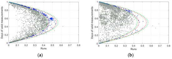
Figure 2.
Totals of 95% (red lines) and 99% (green line) confidence intervals, relating to the randomness of missing data in samples recorded in 2020 (a) and in 2017 (b). Considering the 4266 measured sample and 95% confidence intervals, the time series characterized by random missing data are 24% of the total in 2020 and 7.8% in 2017.
This analysis identifies the time series in which the days of randomly distributed missing data are guaranteed to still provide information on the sample in the registration period. Under these conditions, it is possible to recognize the statistical characteristics and the presence of any periodicity. However, this methodology needs a successive phase of manual control of the results to classify the data, based on the extent and recurrence of the gaps. The use of artificial intelligence appears to be the only viable possibility for an automatic and unsupervised pre-processing of the null measures. In fact, by combining the aforementioned analyses, with a check of the periodicity of the gaps and the holidays foreseen by the calendar, an artificial neural network (ANN) can improve and automate the classification.
The evaluation of the periodic component is performed on the time series defined as representative. The use of the NonUniform Fast Fourier Transform (NUFFT) allows to perform the FFT on sampled signals in the case of non-equispaced sampling. To apply this method the series must be continuous, so the null days are eliminated. However, the information on the presence of gaps remains present in the frequencies assigned to each measurement, which remain unchanged.
The analysis carried out on the measurements of a residential flow meter, which recorded a complete time series in the bimester of the lockdown, is supplied below as an example. In this particular period of measurements, the randomness of consumption is reduced, since those present constantly coincide with the residents. Furthermore, in the case of residents belonging to work categories defined as “non-essential”, the absence of work shifts has limited, or even eliminated, the weekly periodicity.
The first step of this application consists of performing the structural analysis of the complete reference time series, continuously sampled at constant intervals, using FFT.
From this first analysis, the three fundamental frequencies of the sample are identified, which is clearly visible in the power spectrum reproduced in Figure 3a. The main frequency is the daily one, while the other two periodicities are lower than this. For the sample analysed, during the lockdown period, the weekly frequency is not identifiable. The first three harmonics, much larger than the others, are already able to define the main periodic trend of the time series. However, these three harmonics are not able to represent a consistent share of the periodic component of the time series. Analysing the trend of the progressive amplitudes of the analysed sample, a sudden alteration in slope is noted at the 13th harmonic. The 13 significant harmonics are used to develop a periodic model using the inverse Fourier transform (IFT), which returns a reconstructed signal, whose mean is compared to that of the real sample in Figure 3b.
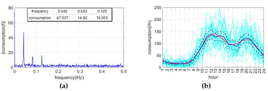
Figure 3.
(a) Power spectrum of the analysed time series; (b) hourly measurements of the measured sample (light blue lines), average value of measured consumptions (blue line), average value of consumptions reconstructed with the 13 significant harmonics (red line) and 95% confidence intervals (black lines).
To prove the stated methodology, the analysed time series has been modified by eliminating an increasing number of daily measurements, highlighted on the complete time series in Figure 4.

Figure 4.
(a) Simulation of a time series with one day of missing data (highlighted in red); (b) simulation of a time series with three consecutive days of missing data (highlighted in green).
On these two incomplete time series, the NUFFT is performed. By comparing the power spectrum obtained on the complete time series (Figure 3a) and the others obtained for samples holding an increasing number of missing data (Figure 4), the three fundamental frequencies are coincident, while the values assumed in correspondence with them is remarkably similar (Figure 5).

Figure 5.
Power spectrum of a sample with (a) one day of missing data or (b) three consecutive days of missing data.
Figure 5 also shows that the presence of an increasing number of days of missing measurements leads to an increasing number of significant harmonics, characterized by a period greater than a day. These harmonics are responsible for the reconstruction of the day of missing measurements within the pseudo-periodic signal. Since the structural analysis was carried out to reconstruct the periodic component of the complete signal, the estimate of the periodic signal is determined with the NUFFT, considering only frequencies higher than the daily one, indicative of the first harmonic. Based on the number of significant harmonics considered, the residuals obtained by subtracting the periodic model from the original demand data can be autocorrelated. For this reason, they need to be tested by an autocorrelation analysis to determine whether they constitute a random sequence. For this purpose, the Ljung–Box test is used, which is frequently used for autocorrelation analyses of time series. This test show that, for this flow meter, no autocorrelation is detected in the stochastic component (Figure 6); therefore, it is possible to statistically characterize the independent residual component.
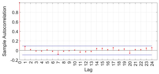
Figure 6.
Sample autocorrelation of the stochastic component. Bounds (blue lines) for α = 0.01.
A fitting of the residuals on probabilistic distributions has identified the three-parameter gamma distribution as the best performing distribution for the time series analysed (Figure 7).
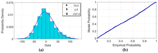
Figure 7.
Fitting of the three-parameter gamma distribution on the stochastic component of the signal. (a) Probability distribution function. (b) Probability–probability plot of the empirical CDF values plotted against the theoretical CDF values.
Once the parameters of the identified distribution are known, the residuals can be generated by the Monte Carlo method. By adding these residues to the periodic component of the signal, a stationary, ergodic, and complete series, relating to the analysed user, is reconstructed.
4. Conclusions and Future Work
The presence of missing measures in a time series is a non-removable problem that prevents the evaluation of the consumption covariance matrix. The impossibility of defining this matrix inhibits the generation of reliable water demand scenarios. For this reason, it is necessary to reconstruct the characteristics of the time series, considering the missing measures. However, extended gaps result in a lack of information that does not allow for the correct characterization of the signal.
The first part of the paper proposed a supervised data pre-processing technique that can help characterize gaps. Then, the authors presented a structural analysis on the incomplete time series. This study confirms that it is possible to efficiently generate the periodic component, starting from incomplete samples. A stationary and ergodic sample can, therefore, be generated from an incomplete series. The comprehensiveness of the data allows the generation of representative consumption scenarios.
Author Contributions
Conceptualization, R.G. and M.M.; methodology, R.G. and M.M.; validation, M.M.; data processing, R.G. and M.M.; resources, G.S.d.U.; data curation, D.F. and G.S.d.U.; writing—original draft preparation, M.M.; writing—review and editing, D.F.; supervision, M.G. and F.D.P. All authors have read and agreed to the published version of the manuscript.
Funding
This research received no external funding.
Institutional Review Board Statement
Not applicable.
Informed Consent Statement
Not applicable.
Data Availability Statement
The data that support the findings of this study are available from Acqua Bene Comune. Restrictions apply to the availability of these data, which were used under license for this study.
Acknowledgments
The authors thank Acqua Bene Comune for having supplied demand data.
Conflicts of Interest
The authors declare no conflict of interest.
References
- Buchberger, S.G.; Wu, L. Model for instantaneous residential water demands. J. Hydraul. Eng. 1995, 121, 232–246. [Google Scholar] [CrossRef]
- Buchberger, S.G.; Wells, G.J. Intensity, duration and frequency of residential water demands. J. Water Resour. Plan. Manag. 1996, 122, 11–19. [Google Scholar] [CrossRef]
- Guercio, R.; Magini, R.; Pallavicini, I. Instantaneous residential water demand as stochastic point process. Water Resour. Manag. 2001, 48, 129–138. [Google Scholar]
- Santopietro, S.; Gargano, R.; Granata, F.; de Marinis, G. Generation of Water Demand Time Series through Spline Curves. J. Water Resour. Plan. Manag. 2020, 114, 04020080. [Google Scholar] [CrossRef]
- Alcocer-Yamanaka, V.H.; Tzatchkov, V.; Buchberger, S.G. Instantaneous Water Demand Parameter Estimation from Coarse Meter Readings. In Proceedings of the Water Distribution Systems Analysis Symposium, Cincinnati, OH, USA, 24–28 July 2006; pp. 1–14. [Google Scholar]
- Creaco, E.; Farmani, R.; Kapelan, Z.; Vamvakeridou, L.; Savic, D. Considering the mutual dependence of the pulse duration and intensity in models for generating residential water demand. J. Water Resour. Plan. Manag. 2015, 141, 557. [Google Scholar] [CrossRef]
- Blokker, E.J.; Pieterse-Quirijns, J.E.; Vreeburg, J.H.; van Dijk, J. Simulating residential water demand with a stochastic end-use model. J. Water Resour. Plan. Manag. 2011, 137, 511–520. [Google Scholar] [CrossRef]
- Magini, R.; Boniforti, M.A.; Guercio, R. Generating Scenarios of Cross-Correlated Demands for Modelling Water Distribution Networks. Water 2019, 11, 493. [Google Scholar] [CrossRef]
- Creaco, E.; Galuppini, G.; Campisano, A.; Franchini, M. Bottom-Up Generation of Peak Demand Scenarios in Water Distribution Networks. Sustainability 2021, 13, 31. [Google Scholar] [CrossRef]
- Morales Martínez, D.; Gori Maia, A. The effect of social behavior on residential water consumption. Water 2021, 13, 1184. [Google Scholar] [CrossRef]
- Padulano, R.; Del Giudice, G. A nonparametric framework for water consumption data cleansing: An application to a smart network in Naples (Italy). J. Hydroinformatics 2020, 22, 666–680. [Google Scholar] [CrossRef]
- Wald, A.; Wolfowitz, J. On a test whether two samples are from the same population. Ann. Math. Stat. 1940, 11, 147–162. [Google Scholar] [CrossRef]
- Leys, C.; Ley, C.; Klein, O.; Bernard, P.; Licata, L. Detecting outliers: Do not use standard deviation around the mean, use absolute deviation around the median. J. Exp. Soc. Psychol. 2013, 49, 764–766. [Google Scholar] [CrossRef]
- Brentan, B.M.; Luvizotto, E.; Herrera, M.; Izquierdo, J.; Perez-Garcia, R. Hybrid regression model for near real-time urban water demand forecasting. J. Comput. Appl. Math. 2017, 309, 532–541. [Google Scholar] [CrossRef]
- Zhao, S.; Wang, C.; Bian, X. Research on harmonic detection based on wavelet threshold and FFT algorithm. Syst. Sci. Control. Eng. 2018, 6, 339–345. [Google Scholar] [CrossRef]
- Chai, X.; Gu, H.; Li, F.; Duan, H.; Hu, X.; Lin, K. Deep learning for irregularly and regularly missing data. Sci. Rep. 2020, 10, 3302. [Google Scholar] [CrossRef] [PubMed]
- Arandia, E.; Uber, J.; Shang, F.; Boccelli, D.; Janke, R.; Hartman, D.; Lee, Y. Preliminary Spatial-Temporal Statistical Analysis of Hourly Water Demand at Household Level. Proceedings of Conference: World Environmental and Water Resources Congress, Kansas City, MO, USA, 17–21 May 2009. [Google Scholar] [CrossRef]
- Dutt, A.; Rokhlin, V. Fast Fourier Transforms for Nonequispaced Data. SIAM J. Sci. Comput. 1993, 14, 1368–1393. [Google Scholar] [CrossRef]
- Potter, S.; Gumerov, N.; Duraiswami, R. Fast Interpolation of Bandlimited Functions. In Proceedings of the IEEE International Conference on Acoustics, Speech and Signal Processing (ICASSP), New Orleans, LA, USA, 5–9 March 2017. [Google Scholar]
- Hartley, H.O. Tests of significance in harmonic analysis. Biometrika 1949, 36, 194–201. [Google Scholar] [CrossRef] [PubMed]
- Shimshoni, M. On Fisher’s test of significance in harmonic analysis. Geophys. J. R. Astr. Soc 1971, 23, 373–377. [Google Scholar] [CrossRef]
- Yevjevich, V. Structural Analysis of Hydrologic Time Series; Colorado State University: Fort Collins, CO, USA, 1972; Volume 56. [Google Scholar]
- Box, G.E.P.; Jenkins, G.M.; Reinsel, G.; Ljung, G. Time Series Analysis: Forecasting and Control, 5th ed.; John Wiley & Sons: Hoboken, NJ, USA, 2015. [Google Scholar]
- Yongkui, L.; Cao, L.; Han, Y.; Shi, Y. Short-Term Electric Load Forecasting with a Hybrid ARIMA, SVR, and IA. In Proceedings of the Methodology Construction Research Congress, Tempe, AZ, USA, 8–10 March 2020. [Google Scholar] [CrossRef]
- Asefa, T.; Adams, A. Short-term urban water demand forecast models in action: Challenges from model development to implementation to real-time operations. In World Environmental and Water Resources Congress 2007; ASCE: Reston, VA, USA, 2007. [Google Scholar]
Disclaimer/Publisher’s Note: The statements, opinions and data contained in all publications are solely those of the individual author(s) and contributor(s) and not of MDPI and/or the editor(s). MDPI and/or the editor(s) disclaim responsibility for any injury to people or property resulting from any ideas, methods, instructions or products referred to in the content. |
© 2022 by the authors. Licensee MDPI, Basel, Switzerland. This article is an open access article distributed under the terms and conditions of the Creative Commons Attribution (CC BY) license (https://creativecommons.org/licenses/by/4.0/).