Estimation of Cloud Water Resources in China

Abstract

With the increasing scarcity of global water resources, the exploitation of atmospheric water resources has emerged as a crucial strategy for mitigating water shortages. However, the development of regional atmospheric water resources remains constrained by the lack of precise atmospheric water resource assessments. Existing studies primarily focus on historical evaluations of atmospheric water resources in China, while future changes in cloud water resources across target regions have yet to be comprehensively investigated. In this study, projections of cloud water resources over China for the next 30 years are conducted based on CMIP6 global climate model simulations, in conjunction with observationally diagnosed cloud water resources datasets from 2000 to 2019. A random forest model, coupled with a fuzzy logic approach, is employed to estimate future cloud water resources, as well as their spatial distribution and temporal trends. The results indicate that the random forest model effectively captures the relationship between atmospheric physical variables and cloud water resources, demonstrating strong agreement with historical data. Over the next three decades, cloud water resources in China are projected to exhibit an overall increasing trend, with the most pronounced enhancement occurring under the high-emission scenario (Shared Socioeconomic Pathway 5–8.5). The spatial distribution pattern of cloud water resources is expected to remain largely consistent with that of the past two decades, while inter-model differences are primarily observed in southeastern China and the southern Tibetan Plateau. Further analysis using fuzzy logic inference reveals that the most significant increases in cloud water resources are anticipated in northwestern China, with the potential for an expansion of these increases toward the north under the high-emission scenario. This study provides a scientific framework for predicting future variations in cloud water resources across China, offering critical theoretical and data-driven support for the sustainable development and utilization of atmospheric water resources.

1. Introduction

Amid increasing freshwater scarcity, the utilization and development of atmospheric water resources have become crucial strategies for alleviating water shortages. China, as one of the most extensively engaged nations in weather modification operations, faces uncertainties in regional-scale atmospheric water resource development due to the lack of precise assessments of exploitable atmospheric water resources [1].

The exploration of cloud water resources (CWRs) internationally began with water vapor monitoring. Benton et al. [2] utilized radiosonde and wind profile data to calculate the total water vapor transport at individual stations. In China, research on atmospheric water resources began in the 1980s. Lu [3] analyzed the annual and monthly atmospheric water vapor content and transport over China during the 1970s using upper-air station data. With the advent of meteorological satellites providing cloud observations, research shifted towards assessing atmospheric cloud water content. Greenwald et al. [4] and Li et al. [5] conceptualized cloud water content as “cloud water resources” and conducted studies at both global and regional scales over China.

In recent years, the rapid development of atmospheric reanalysis datasets—offering broad spatial coverage, high temporal continuity, and long historical records—has enabled extensive studies on water vapor and cloud water resources across various regions in China [6,7,8]. Most previous studies have focused on the state variables of atmospheric water, such as water vapor content and transport, to evaluate cloud water resources. However, treating water vapor as the primary form of atmospheric cloud water resources may lead to overestimation. This overestimation arises because water vapor does not directly convert into precipitation; it must first transit into hydrometeors before undergoing cloud microphysical processes and gravitational settling to reach the surface. Moreover, compared to state variables, the advection and associated sources and sinks of hydrometeors play a more critical role in regional atmospheric water cycles and cumulative precipitation over specific timeframes.

Zhou et al. emphasized hydrometeors as the core component of cloud water resource assessments. In 2011, they initiated the cloud water resource monitoring and estimating methodology and later formally defined cloud water resources as “the total amount of hydrometeors remaining in the atmosphere within a specific spatial and temporal range that has participated in the atmospheric water cycle but has not yet precipitated” [9]. This led to the development of quantitative assessment methods based on observational diagnostics and numerical simulations. Using these methods, they evaluated cloud water resources over North China for 2015–2019 and conducted consistency tests between different assessment approaches [10,11]. Cai et al. produced high-resolution datasets, including a 1° × 1° global and China cloud water resource dataset from 2000–2019, a 2.5° global dataset spanning 1960–2019, and a 3 km-resolution numerical simulation dataset for North China from 2015–2019 [10].

These datasets have facilitated new insights into the physical characteristics and spatiotemporal distribution of atmospheric water cycles and cloud water resources. Key findings include: over the past two decades, cloud water resources over global land areas have been concentrated in cold regions of the Köppen climate classification system at mid-to-high latitudes; with global warming, terrestrial cloud water resources have exhibited an overall increasing trend [12]; in China, the annual mean cloud water resource amount is approximately 176.4 mm, with significant regional differences. When dividing China into six regions, the ranking from highest to lowest cloud water resource amount is as follows: Southeast, Central, Southwest, Northeast, North China, and Northwest [13].

Furthermore, recent studies have identified notable trends in cloud water resources over China. In the Tibetan Plateau, major river basins exhibit a “dry-getting-drier, wet-getting-wetter” pattern, with increasing CWR trends in the Yellow River and Yangtze River basins [14]. Additionally, in the climate-sensitive Northwest region, overall CWRs has shown an increasing trend, particularly in spring, suggesting greater seasonal development potential [15]. Temporal and spatial characteristics of cloud water resources have also been investigated [9,11].

However, the above research on cloud water resources remains at the level of analyzing historical data. To understand how the climate state of cloud water resource distribution patterns and corresponding trends will change in China and even globally in the near- to mid-term future, a reasonable forecasting approach is needed. Zhou et al. [9] evaluated cloud water resource observations and numerical methods, both of which are based on solving the water balance equation. This approach benefits from the completeness of historical data, as atmospheric reanalysis datasets from past periods assimilate satellite and ground-based observations, with pressure levels reaching up to 31 layers. However, future datasets may contain only a limited number of pressure levels.

Machine learning methods are often used to evaluate complex nonlinear relationships between a limited number of independent variables [16]. Therefore, they can capture key atmospheric variables and their physical relationships with cloud water resources in historical datasets, serving as an alternative to traditional equation-based approaches for evaluating cloud water resources. With a fundamental model established, it is also necessary to provide future atmospheric variable data, and global climate models (GCMs) offer this possibility.

Global climate models provide a detailed representation of atmospheric dynamics, heat exchange, and land–sea–ice–atmosphere interactions over time [17] and serve as effective tools for assessing the impact of atmospheric changes on the Earth’s surface in past, present, and future scenarios [18,19]. The Coupled Model Intercomparison Project Phase 6 (CMIP6) represents the latest initiative for climate projections, offering improved experimental designs and higher resolutions compared to Coupled Model Intercomparison Project Phase 5(CMIP5), thereby enhancing global and regional climate studies [20]. Additionally, CMIP6 introduces new future projection scenarios based on shared socioeconomic pathways (SSPs) and representative concentration pathways (RCPs), incorporating diverse air pollutant emission scenarios to provide more comprehensive simulations for climate change mechanisms and adaptation strategies [21]. CMIP6 data have been widely used for regional and global climate projections, including studies on temperature, precipitation, runoff, and future extreme events [22,23,24,25,26,27,28,29,30]. Cloud-related research based on CMIP6 has also been conducted, covering aspects such as cloud radiative effects [31], total cloud cover [32,33], and cloud feedback mechanisms [34]. The Cloud Feedback Model Intercomparison Project (CFMIP) has been established as a subproject of CMIP6 [35].

Based on the above, to study how the distribution and trends of cloud water resources in China will change under different climate backgrounds in the mid-to-short term future, this paper proposes a scheme for estimating cloud water resources in the region. This scheme is based on the cloud water resource estimates provided by Zhou et al. [9]’s observationally diagnosed dataset for China from 2000 to 2019. A machine learning approach is used to fit the physical relationship between atmospheric variables and cloud water resource estimates over the past two decades. The trained model is then combined with atmospheric parameters from CMIP6 global climate models to project the climatic distribution of cloud water resources in China for 2025–2054. The projections from multiple climate models are further processed using a fuzzy logic method to obtain a comprehensive trend distribution. Through this estimation scheme, the distribution characteristics and variation trends of cloud water resources in China over the next 30 years under two emission scenarios are obtained. This study aims to provide a scientific reference for the rational development of atmospheric water resources and addressing water scarcity issues in China.

2. Datasets and Methods

2.1. Cloud Water Resource Observational Diagnostic Assessment Dataset

To compute the cloud water resource assessment variables and other related physical quantities, it is essential to obtain the raw data fields of the cloud water resource observational diagnostic assessment dataset. This includes three-dimensional atmospheric temperature, water vapor, cloud water, and precipitation fields for the historical period from 2000 to 2019.

The water vapor field is derived from the NCEP/NCAR Final Analysis (FNL) atmospheric reanalysis dataset [36], which provides a three-dimensional representation of water vapor and the budget of water vapor in the horizontal and vertical directions at different pressure levels, with a spatial resolution of 1° × 1° and four daily timestamps (00:00, 06:00, 12:00, and 18:00 UTC). The precipitation field originates from the 1° × 1° Global Precipitation Climatology Project (GPCP) dataset [37,38].

Additionally, a time-varying three-dimensional cloud water field is required, representing the spatial distribution of cloud water content across longitude, latitude, and altitude. Cai et al. [39] proposed a method for diagnosing cloud regions based on atmospheric thermodynamic profiles using satellite and aircraft observations to establish the relationship between cloud occurrence and atmospheric temperature-humidity conditions. They employed the threat score (TS) method to statistically determine the relative humidity threshold profile for diagnosing cloud presence. Using diagnosed cloud regions and the vertical distribution profile of cloud water content, combined with the temporally and spatially continuous three-dimensional temperature and humidity fields from the NCEP/NCAR reanalysis dataset, it is possible to derive the time-varying three-dimensional spatial distribution of cloud water. This dataset provides cloud water content, as well as the budget of hydrometeors in the horizontal and vertical directions, at different pressure levels with a 1° × 1° resolution at four daily timestamps (00:00, 06:00, 12:00, and 18:00 UTC).

Based on the initial meteorological data fields above, the corresponding characteristic variables in the Cloud Water Resource Diagnosed Assessment Dataset (hereafter referred to as CWRs-DAD) for the study period can be calculated using Equations (1)–(3). These include the cloud water resource estimates (hereafter referred to as CWRs).

$$M_{v1}+Q_{vi}+C_{hv}+E_s=M_{v2}+Q_{vo}+C_{vh},$$

(1)

$$M_{h1}+Q_{hi}+C_{vh}=M_{h2}+Q_{ho}+C_{hv}+P_s,$$

(2)

$$M_{w1}+Q_{wi}+E_S=M_{w2}+Q_{wo}+P_s,$$

(3)

$$\begin{array}{c}\mathrm{CWRs}=Q_{hi}+C_{vh}+M_{h1}-P_s\\ =Q_{ho}+C_{hv}+M_{h2}\end{array}$$

(4)

Equation (1) represents the water vapor budget equation, Equation (2) represents the hydrometeor budget equation, and Equation (3) represents the water substance (water vapor and hydrometeors) budget equation. The final Equation (4) is the calculation formula for the cloud water resource evaluation. In these equations, v denotes water vapor, h denotes hydrometeors, and w denotes water substance. $M_{v1}$ and $M_{v2}$ represent the initial and final state values of cloud water content during the study period; similarly, $M_{h1}$ and $M_{h2}$, as well as $M_{w1}$ and $M_{w2}$, represent their respective state values. $Q_{vi}$ and $Q_{vo}$ denote the input and output values of water vapor advection within the region; likewise, $Q_{hi}$ and $Q_{ho}$, and $Q_{wi}$ and $Q_{wo}$ represent the advection terms for the respective water substances. $E_s$ and $P_s$ represent the surface evaporation and precipitation, which serve as the source and sink terms within the region, while $C_{vh}$ and $C_{hv}$ denote the condensation of water vapor into hydrometeors and the evaporation of hydrometeors into water vapor, respectively. Considering data intuitiveness, the computational results are uniformly expressed in mm (equivalent to kg·m⁻²). For further details on the calculations of additional physical quantities, see Zhou et al. [9].

To validate the reliability of this dataset, Zhou et al. and Cai et al. conducted a cloud water resource diagnostic assessment for typical months in the North China region based on the 1° × 1° CWRs-DAD. Additionally, they employed the Cloud Precipitation Explicit Forecast System (CPEFS) model to perform a numerical assessment of cloud water resources over the same period and region, obtaining a numerical assessment result with a resolution of 3 km. A comparative analysis of the two assessment methods demonstrated a fine degree of consistency between their results [11].

In this study, the CWRs from CWRs-DAD are used as ground truth references. It is worth noting that, since the CWRs-DAD data span from 2000 to 2019, with the forecast period being 2025–2054 and the 2020–2024 period being a missing segment in the historical data, this does not affect the model training. The dataset, consisting of tens of millions of data points from the past 20 years, is sufficient for machine learning models.

2.2. Coupled Model Intercomparison Project Phase 6 (CMIP6)

To promote model development and enhance scientific understanding of the Earth’s climate system, the World Climate Research Programme has hosted six phases of the Coupled Model Intercomparison Project. The ongoing sixth phase, CMIP6, consists of three levels of model experiments, with the core experiment being the DECK (Diagnostic, Evaluation, and Characterization of Klima) experiment [40].

Within the CMIP6 model comparison sub-programmes, there is the Scenario Model Intercomparison Project (ScenarioMIP). Climate projections under different scenarios have been a core component of previous IPCC scientific assessment reports. The results of these projections reveal the climate impacts and socioeconomic risks associated with various policy choices, making them an essential scientific basis for policy decisions. ScenarioMIP generates quantitative emissions of temperature- and humidity-related gases, atmospheric components, and land use changes based on different shared socioeconomic pathways (SSPs), thus producing scenario-based projections. SSP5-8.5 represents a socioeconomic pathway that leads to a radiative forcing of 8.5 W/m² by 2100, while SSP2-4.5 represents a middle-ground scenario with radiative forcing of 4.5 W/m², corresponding to moderate socioeconomic vulnerability [41].

The models used in this study include ACCESS-CM2(Australian Community Climate and Earth-System Simulator Climate Model version 2), ACCESS-ESM1-5(Australian Community Climate and Earth-System Simulator Earth System Model version 1.5), BCC-CSM2-MR(Beijing Climate Center Climate System Model version 2 with Medium Resolution), CanESM5(Canadian Earth System Model version 5), EC-Earth3(EC-Earth Model version 3), FGOALS-g3(Flexible Global Ocean-Atmosphere-Land System Model version g3), INM-CM4-8(Institute of Numerical Mathematics Climate Model version 4.8), and MPI-ESM1-2-HR(Max Planck Institute Earth System Model version 1.2 High Resolution). These climate models are commonly used for future climate change research, with their data summarized in

Table 1. Introduction to climate models.

Model Name	Country/Institution	Grid Size
ACCESS-CM2	Australia, Australian National University	144 × 192
ACCESS-ESM1-5	Australia, Australian National University	144 × 192
BCC-CSM2-MR	China, Beijing Climate Center	160 × 320
CanESM5	Canada, Canadian Environmental Assessment Agency	64 × 128
EC-Earth3	EU, European Centre for Medium-Range Weather Forecasts	256 × 512
FGOALS-g3	China, Institute of Atmospheric Physics, Chinese Academy of Sciences	80 × 180
INM-CM4-8	Russia, Institute of Numerical Mathematics, Russian Academy of Sciences	120 × 180
MPI-ESM1-2-HR	Germany, Max Planck Institute for Meteorology	192 × 384

. Considering that greenhouse gas emissions remain high, the socioeconomic scenarios used are the moderate emission scenario SSP2-4.5 and the high emission scenario SSP5-8.5, with the initial model conditions set to r1i1p1f1. The time frame selected for the study is 2025–2054, with data on a daily scale, and the specific physical quantities considered include surface temperature, atmospheric temperature, precipitation, wind fields, and specific humidity. The selected pressure levels are 250 hPa, 500 hPa, 700 hPa, and 850 hPa. Additionally, cloud water resources are directly linked to precipitation [9], and these models are well-suited for precipitation simulation in the China region.

2.3. Random Forest

2.3.1. Introduction to Random Forest

The basic idea and concept of random forest (RF) were proposed by Ho [42], and were later refined by Breiman [43] to form the final RF algorithm. Han et al. [44] further discovered that RF can outperform neural networks under conditions of low sample sizes. With the development of research, the RF algorithm has been advanced and applied in various fields. The RF model, with its high prediction accuracy and ease of tuning, has become a widely favored ensemble method among researchers. It solves the limitation of single decision tree expressions, and ensemble learning tends to perform better than individual classification models. Additionally, the randomness in sample selection and feature selection during the training process further ensures its generalization capability. As a result, the RF model has good applicability for predictions. In this study, the RF model was selected to fit the physical relationships between multiple atmospheric variables and cloud water resources evaluation quantities.

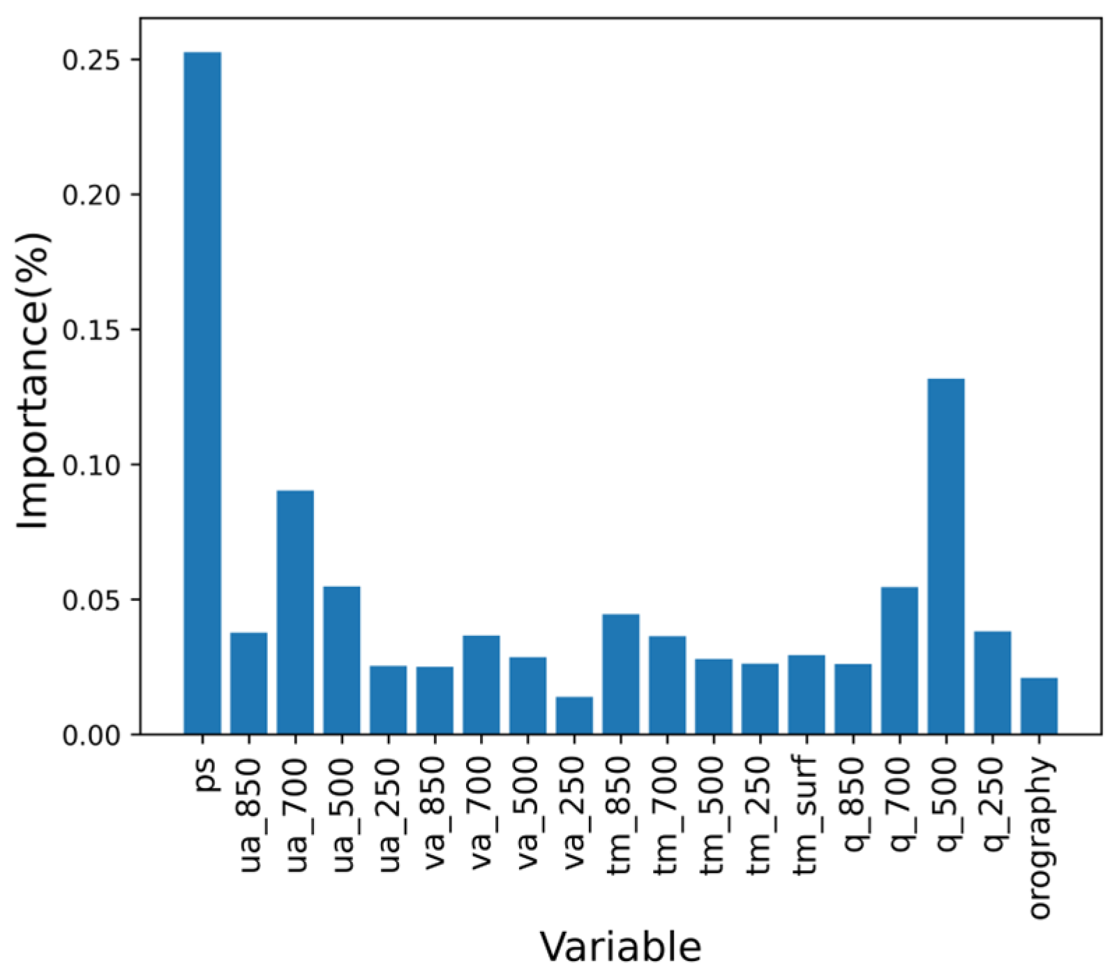
2.3.2. Feature Selection

The primary task of machine learning is to create a training dataset. The main data source for the training dataset in this study is the NCEP FNL atmospheric reanalysis data from 2000 to 2019. The purpose is to directly fit the relationship between atmospheric variable data and cloud water resources evaluation quantities, replacing traditional equation solving methods. The training data used for model training and validation consist of the cloud water resources diagnostic dataset and the NCEP FNL dataset, while the CMIP6 model data form the input dataset for the predictions.

In preparing the training dataset, feature parameters must be selected. It is known that the cloud water resources dataset is generated through processing of the FNL data, mainly using the temperature, humidity, and wind fields from FNL to generate the corresponding three-dimensional cloud water and water vapor fields. Therefore, surface temperature, atmospheric temperature, specific humidity, and horizontal and vertical wind field were selected as features. Considering the complex terrain of the China region, the geopotential height was also included as one of the feature parameters. Finally, since the physical meaning of CWRs is directly related to precipitation, the GPCP precipitation data was chosen as the final feature. The cloud water resource amount from CWRs-DAD were used as true values. Based on the above, the selected feature parameters were: atmospheric temperature, surface temperature, specific humidity, horizontal and vertical wind field, geopotential height, and precipitation. Figure 1 shows the feature parameter importance map after training, where the physical quantity with the highest influence weight is precipitation, which is closely related to the physical definition of cloud water resources as the total condensing material minus natural precipitation.

2.3.3. Preprocessing

During the creation of the dataset, due to inconsistencies in the temporal and spatial resolutions of the data, matching processing is required. The corresponding processing steps are described below.

Vertical Resolution: As previously mentioned, the cloud water resources evaluation values used in this study are calculated from the atmospheric moisture balance equation. The initial data fields consist of three-dimensional cloud water and water vapor fields, which have 26 layers of pressure levels. However, the CMIP6 climate model datasets only have 8 layers, which are 1000 hPa, 850 hPa, 700 hPa, 500 hPa, 250 hPa, 100 hPa, 50 hPa, and 10 hPa. Considering that water vapor above 200 hPa in the atmosphere is relatively scarce compared to the lower layers, we select the physical quantities corresponding to the 250 hPa, 500 hPa, 700 hPa, and 850 hPa pressure levels.

Spatial Resolution: The spatial resolution of various model data in CMIP6 is inconsistent. To unify the input data for the random forest model, they must be standardized to the spatial resolution of the FNL dataset. The method used here is bilinear interpolation, which adjusts the resolution of all model data to 1° × 1° within the region 70.5° E to 140.5° E and 15.5° N to 55.5° N.

Temporal Resolution: Precipitation data are already in accumulated form, but for non-accumulated quantities such as temperature, specific humidity, and wind speed, a weighted average is required. The temporal resolution of the FNL (final analysis) atmospheric reanalysis data is 6-hour intervals, with 4 time steps per day. We calculate the daily average temperature, wind speed, and specific humidity by creating a weighted average. Since the CMIP6 data are already on a daily scale, no special processing is needed. Figure 2 shows the entire data preprocessing process.

2.3.4. Model Parameter Selection and Optimization

The model training is based on the RandomForestRegressor from the Scikit-Learn library in Python. The prediction performance of the model is significantly influenced by the selection of hyperparameters, and we use a stepwise method to select the optimal hyperparameters. Among these, the number of decision trees is one of the key factors affecting the forecast accuracy. A higher number of trees indicates stronger data fitting ability. However, increasing the number of trees indiscriminately can lead to a large memory footprint for the model. Therefore, considering the size of the dataset, the number of trees (n_estimators) is chosen in the range of (50, 100) with a step of 1. Feature selection at the decision tree nodes is another important model parameter. By splitting data at the node, the information entropy at that node is reduced. The maximum number of features (max_features) can be selected as either ‘auto’ or ‘sqrt’. The greater the maximum depth of a single decision tree, the more leaf nodes it will have, which allows for finer fitting of the training data. To avoid overfitting, the maximum tree depth (max_depth) is set in the range of (50, 200) with a step size of 2. The minimum number of samples required to split a node (min_samples_split) can limit tree growth, thus preventing overfitting and improving generalization ability. In this study, the min_samples_split can be selected as 1, 2, 4, or 9. To ensure reproducibility of the experiment, the random seed is set to 42.

These hyperparameters were tested 100 times with random selection within the specified ranges. Through 3-fold cross-validation, the optimal hyperparameter combination was found as follows: n_estimators = 96, min_samples_split = 2, max_features = ‘sqrt’, max_depth = 87, max_features = ‘auto’.

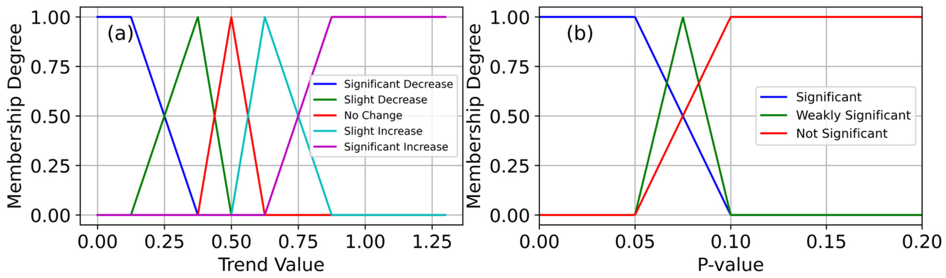
2.4. Fuzzy Logic Algorithm

The fuzzy logic algorithm is a mathematical method based on fuzzy set theory, used to process fuzzy or uncertain information. Compared with traditional binary logic, fuzzy logic involves vagueness, uncertainty, and partial truth. It primarily introduces a membership function to describe the degree of belonging to a certain fuzzy set, where the membership value ranges from 0 to 1, representing the degree of belonging to a specific fuzzy set. Fuzzy logic is widely used in control systems, decision support systems, pattern recognition, and artificial intelligence. In meteorology, it is also commonly applied to tasks such as identifying different radar echoes from objects, hail characteristic discrimination, cloud phase [45], and precipitation particle recognition [46,47,48]. This study uses fuzzy logic algorithms to integrate the trend distributions of eight global climate models, providing possible trend changes in cloud water resource evaluation in different regions of China in the future.

In this study, the input parameters for the fuzzy logic inference, in addition to the trend values calculated by the climate models, also include the p-values from significance testing. Since the range of trend values differs significantly among the different climate models, the trends are first scaled to a standard range, such as scaling to the interval [−1,1]. However, to avoid the additional interference that positive and negative values might bring to subsequent averaging, all trend values are confined to the range of 0 to 1. A value in [0, 0.5] represents a negative trend, [0.5, 1] represents a positive trend, and 0.5 indicates no trend. The p-value range is from 0 to 1, so no additional processing is needed. The fuzzy sets for the trend values are: “Significant Increase”, “Slight Increase”, “No Change”, “Slight Decrease”, and “Significant Decrease”, while the fuzzy sets for the p-values are: “Significant”, “Weakly Significant”, and “Not Significant”. Figure 3a shows the membership function for the trend values, and Figure 3b shows the membership function for the p-values.

3. Results

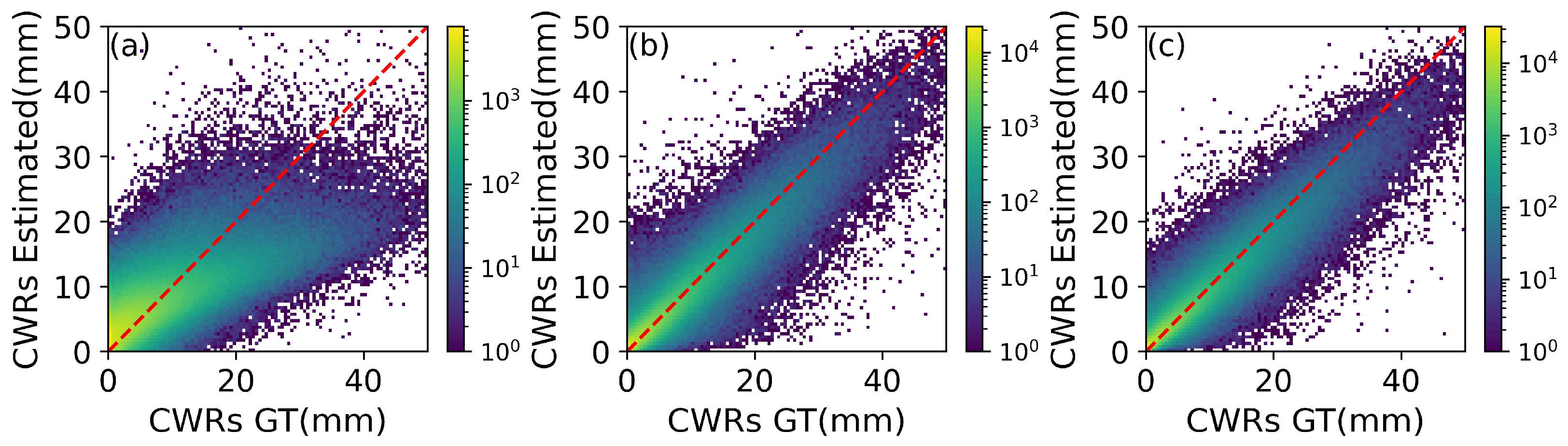
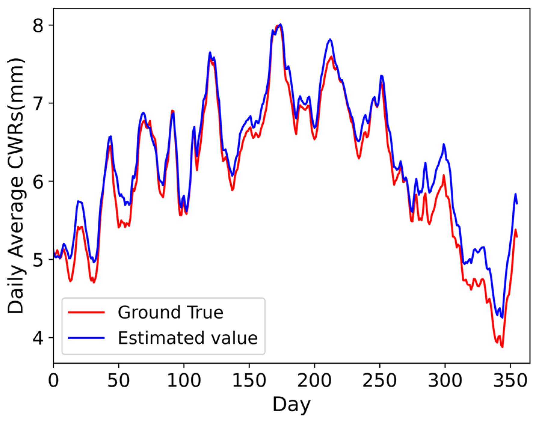
3.1. Model Validation Results

To validate the effectiveness of the trained random forest model in predicting cloud water resources, training data prepared as described in Section 2.3.3 were used as input for the random forest model. The sample dataset consists of a total of 20,944,645 records. Given the large size of the dataset, training the model with all data would result in excessive computational load and time consumption, even with optimized model parameters. Therefore, a random sample of 4 million records was selected for training. Of these, 80% of the data were used for training the random forest model to fit the relationship between atmospheric multi-parameters and the target physical variable (i.e., CWRs), while the remaining 20% served as the testing set.

To compare the fitting ability of the random forest model for cloud water resource estimates, Figure 4 presents the two-dimensional(2D) histograms of the fitting results from the regularized statistical regression model, neural network, and random forest model on the test set. All three models are optimized, with the statistical regression model having a learning rate of 0.01, the neural network model having 256 neurons in both the input and hidden layers, 1500 training iterations, and a random seed of 42. From the 2D histograms in Figure 4 and the evaluation metrics in

Table 2. Model evaluation metrics.

	RMSE *	MAE *	CC *
Statistical Regression	4.71	3.34	0.72
Neural Network	2.63	1.73	0.92
Random Forest	2.42	1.57	0.94

* RMSE is the root mean square error, MAE is the mean absolute error, and CC is the correlation coefficient.

, it is evident that the random forest model has the smallest error among the three models, and its fitting performance outperforms the other two models. Specifically, for the random forest results (Figure 4c), the overall model fitting performance is quite good. Generally, the values of cloud water resource estimates are concentrated in the lower range, with most of the data samples clustered along the diagonal. The linear relationship between the model’s predicted values and the ground truth (GT) values is relatively clear.

To further test the fitting performance of the random forest model, the training dataset for the entire year of 2005 was selected as the input, and the model’s CWRs assessment results for that year were output. Figure 5 presents the daily variation series of the CWRs averaged over grid points in China for the year 2005, as predicted by the model. It can be observed that the model’s estimated CWRs values exhibit a trend consistent with the GT values on a daily timescale, although the predicted values are generally overestimated. This phenomenon is related to the model’s tendency to overestimate in the lower value range.

Figure 6 compares the model’s output of CWRs distribution for April 10 and June 9, 2005, with the original dataset. It is evident that the distribution of the model’s output closely matches the GT distribution, with both high and low value regions being accurately distinguished. However, in the lower value areas of the GT distribution, the model tends to slightly overestimate the CWRs values, which aligns with the previous analysis.

In conclusion, compared to the statistical regression model and the neural network model, the random forest model better fits the relationship between temperature fields, precipitation fields, three-dimensional wind fields, terrain elevation fields, humidity fields, and CWRs.

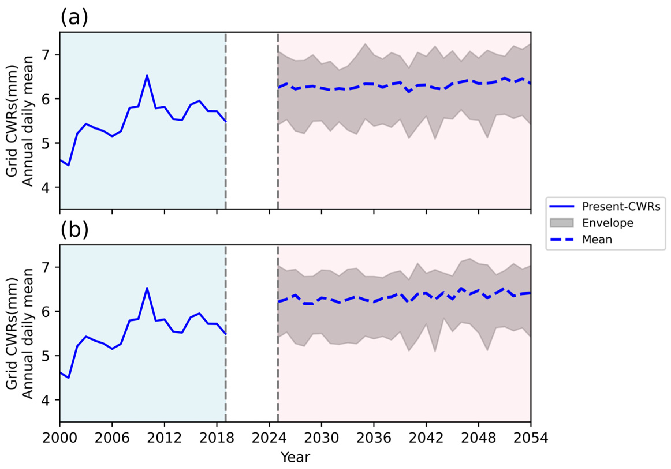
3.2. Interannual Variation Trends of Cloud Water Resources for the Next 30 Years

The previous section discussed how the RF model effectively fits the physical relationships between multiple atmospheric variables and CWRs. This section utilizes the trained model to forecast the changes in cloud water resource assessments for the period 2025–2054 under different socioeconomic pathways in China.

Figure 7 presents the variation curves of the daily average and grid-averaged cloud water resource assessments (hereafter referred to as CWRs-Mean) for the years 2000–2019 and 2025–2054 in China. Over the past 20 years, CWRs-Mean in China has shown a significant increase. For the next 30 years, CWRs-Mean exhibits substantial fluctuation across different climate model outputs. The multi-model average results indicate a slight increase compared to the past two decades.

Table 3. CWRs-Mean trend results of multiple climate models under different scenario modes.

Scenario Mode	Climate Model	CWRs-Mean Trend (mm/a)
SSP2-4.5	ACCESS-CM2	0.0031
	ACCESS-ESM1-5	0.0041
	BCC-CSM2-MR	0.0085
	MPI-ESM1-2-HR	0.0024
	FGOAL-g3	0.0050
	INM-CM4-8	0.0053
	EC-Earth3	0.0054
	CanESM5	0.0055
SSP5-8.5	ACCESS-CM2	0.0064
	ACCESS-ESM1-5	0.0095
	BCC-CSM2-MR	0.0085
	MPI-ESM1-2-HR	0.0082
	FGOAL-g3	0.0001
	INM-CM4-8	0.0077
	EC-Earth3	0.0126
	CanESM5	0.0082

presents the CWRs-Mean trends for the eight climate models under the SSP2-4.5 and SSP5-8.5 scenarios. In all scenarios and across all global climate models, CWRs-Mean demonstrates an increasing trend. Additionally, for the same climate model, the increase in CWRs-Mean under the SSP5-8.5 scenario is generally stronger than that under the SSP2-4.5 scenario.

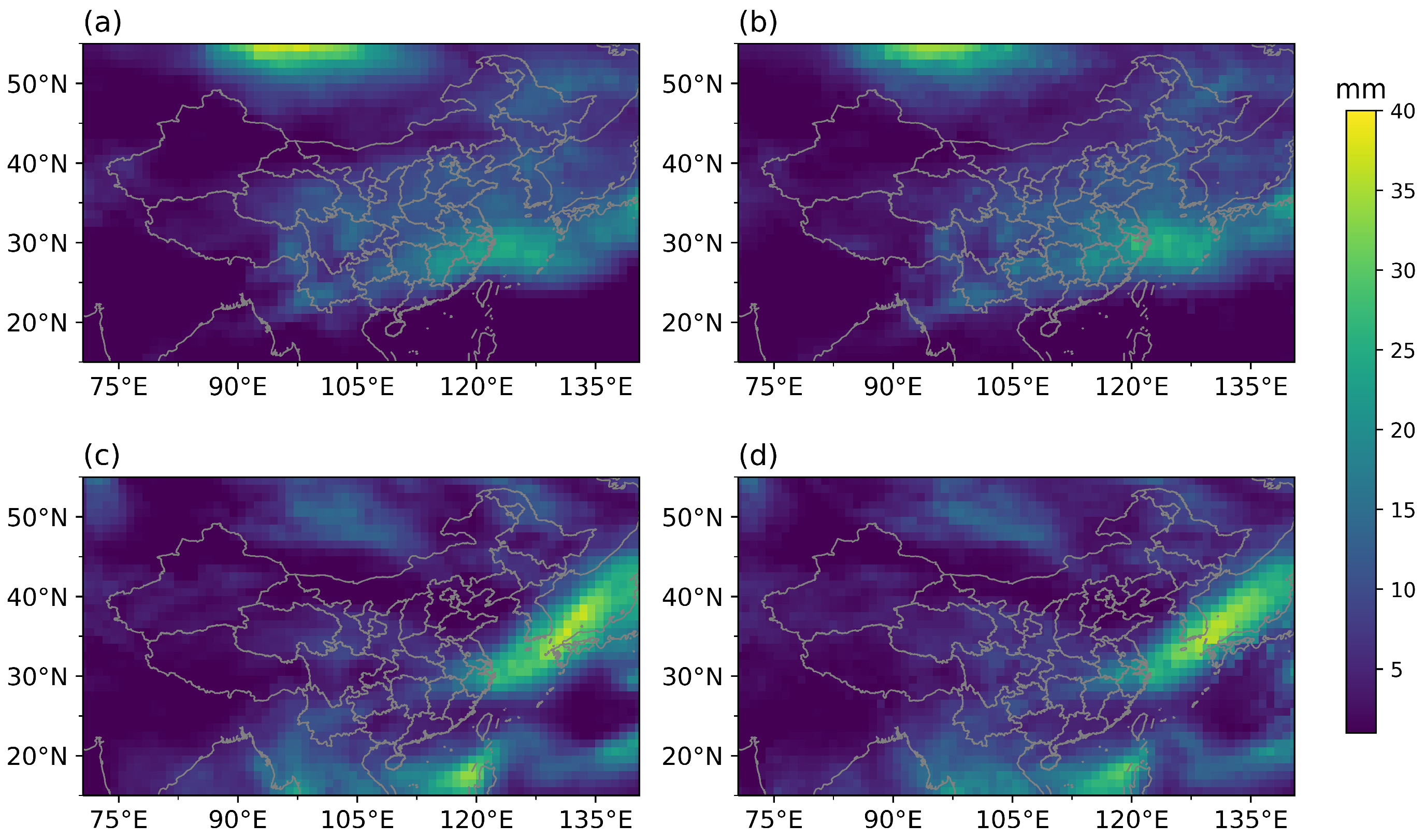
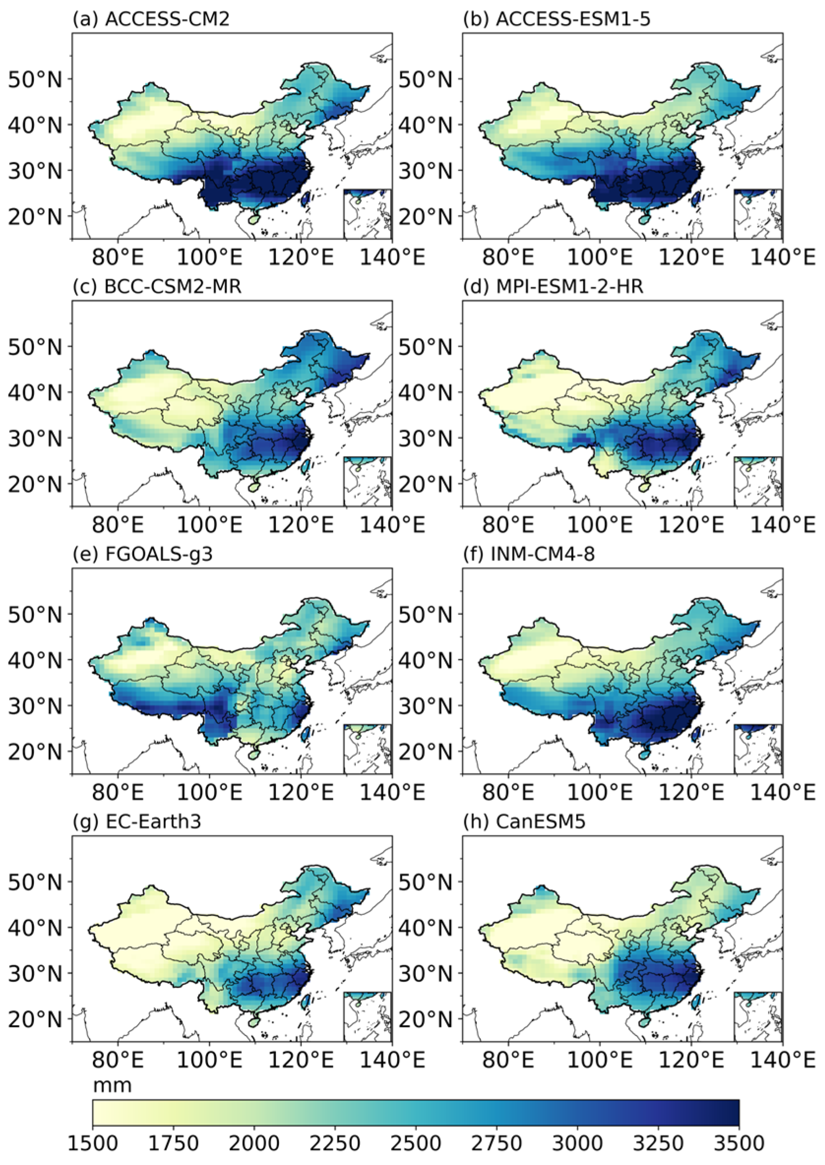
3.3. Distribution and Changes of Cloud Water Resources-Related Quantities for the Next 30 Years

Section 3.2 has already indicated that the overall cloud water resource assessments in China are projected to increase over the next 30 years (2025–2054). An important focus of this section is to investigate how the distribution of cloud water resources in the next 30 years will differ from that of the past 20 years (2000–2019) under different emission scenarios. Figure 8 and Figure 9 show the different performances of CWRs under the SSP2-4.5 and SSP5-8.5 scenarios across eight climate models, with the distributions representing multi-year averages.

From the distribution results under the SSP2-4.5 or SSP5-8.5 scenarios, although there are regional differences, the overall trend shows that CWRs are most abundant in the southeast of China, followed by the northeast, with the northwest being the lowest. However, there is no significant difference in CWRs results for the same climate model under different scenarios. Compared to the CWRs over the past 20 years, the average projections from these eight models for the next 30 years (see Figure 10) remain generally consistent, suggesting that the Tibetan Plateau may have more abundant cloud water resources in the future. However, there are significant differences among the model projections for cloud water resources over the Tibetan Plateau.

Figure 11 and Figure 12 show the projected changes in CWRs for China over the next 30 years under the SSP2-4.5 and SSP5-8.5 scenarios, respectively, based on predictions from eight global climate models. As mentioned in the previous section, the annual average distribution results for the same model show little difference between the two scenarios; however, the trend distribution maps reveal very distinct differences between the two scenarios.

Figure 11 shows the distribution of CWRs trend results under the SSP2-4.5 scenario. Overall, more grid points tend to indicate an increasing trend, with these areas mostly appearing in the western and southern regions. Figure 12 presents the trend distribution under the SSP5-8.5 scenario. Compared to SSP2-4.5, SSP5-8.5 exhibits a greater number of grid points where CWRs show an increasing trend. This also explains why the overall increase in SSP5-8.5 is more pronounced than in SSP2-4.5, as shown in Table 3. Additionally, under this scenario, the differences in trends among various models become more prominent.

Different global climate models have provided varying projections of cloud water resource trends across China, with significant differences among the results. To establish a unified trend distribution and enable a more intuitive assessment of future CWRs changes in China, fuzzy logic inference is applied to the trend distributions of the eight global climate models under the two emission scenarios.

Table 4. Decision rule weights.

Trend\P	Significant Increase	Weak Increase	No Change	Weak Reduction	Significant Reduction
Significant	0.9	0.7	0.5	0.3	0.1
Weak Significant	0.9	0.7	0.5	0.3	0.1
Non Significant	0.7	0.5	0.5	0.5	0.3

presents the weight allocation of the decision rule system, where the weights are assigned based on the membership functions of trend values and p-values. This ensures that the final judgment is derived under different fuzzy sets of significance p-values and trend values. For each grid point within the region, the results from the eight global climate models are available, resulting in eight sets of arrays formed by the combination of trend values and p-values. Each set is processed by the decision system, which outputs a unique composite trend value. These eight composite trend values are then weighted and averaged to generate the comprehensive trend distribution shown in Figure 13.

From the results in Figure 13, it can be observed that the comprehensive trend distribution of CWRs under both SSP2-4.5 and SSP5-8.5 scenarios is predominantly increasing, which is consistent with the analysis in Table 3. Specifically, under SSP2-4.5, the probability of cloud water resource increases is higher in northwestern China and the southwestern region where the Tibetan Plateau is located, while the northeastern region tends to show a decline. Under SSP5-8.5, regions with an increasing trend, such as the Tibetan Plateau, exhibit a more pronounced increase compared to SSP2-4.5. Additionally, the areas experiencing increases extend further northward, reaching even the northeastern regions, while the southeastern region shows a more significant decreasing trend.

The forecasted trends for CWRs over the next 30 years (Figure 13a,b) align with the changes observed over the past 20 years (Figure 13c). Both suggest that the northwest region will continue to experience an increase in cloud water resources, while under moderate emission scenarios (SSP2-4.5), the southeast and northeastern regions may shift from an increasing trend to a decreasing one, particularly in the northeast. Under high emission scenarios (SSP5-8.5), the southwest region is likely to maintain growth in CWRs, while the northeastern region may still experience a decline.

Overall, the areas where cloud water resources increased over the past 20 years are concentrated in the northwest and the southeastern coastal regions. In the next 30 years, the northwest will remain a zone of increased CWRs, with the Tibetan Plateau experiencing particularly pronounced growth. As emissions increase, the region of increased CWRs may expand northward.

4. Discussion

4.1. Model Bias

Regarding the model’s fitting error, although a comparison of models has already been made, indicating that the random forest model has certain advantages, there remains some overestimation. This overestimation mainly arises from the model’s tendency to overestimate the smaller values of CWRs. While the model generalizes well across the entire value range, it performs less effectively for smaller values. Additionally, the dataset contains a relatively high number of small value samples. For example, as shown in Figure 14, CWRs less than 1 mm account for 19% of the training samples. As a result, the cumulative estimation error leads to an overall higher bias. Future work will consider using piecewise regression prediction methods to optimize the small value range and reduce this error.

4.2. Uncertainty Analysis of the Forecasting Results

In this study, data from eight different global climate models (GCMs) were used. These eight models are commonly used for projecting future climate factors in China. However, these models differ in their ability to simulate historical climate and forecast future climate conditions [41,49]. The following shows the evaluation results of the annual daily average surface temperature and precipitation for the historical period of 2000–2014 in China from these eight GCMs, with temperature data from the observational NCEP-FNL dataset and precipitation data from GPCP. From Figure 15, it is evident that the precipitation simulation abilities of the eight models are relatively similar in terms of absolute error and correlation, but there are significant differences in the standard deviation ratio. This indicates that the models differ in their ability to simulate extremes. For temperature simulation, the results show that the models have similar capabilities.

The differences in simulation results can be attributed to several factors. First, there are key differences in the physical parameterization schemes between the models, including convection schemes, cloud microphysics methods, and radiation schemes [21]. The convection scheme determines how the model simulates the precipitation process, leading to differences in precipitation simulation results. The cloud microphysics scheme affects the simulation of cloud droplets and ice crystals, and the radiation scheme impacts shortwave and longwave radiation, which in turn influences temperature differences. In addition, differences in the coupled sea–land–atmosphere climate systems between models, particularly the impact of land surface models on surface temperature, contribute to the variations.

Furthermore, it should be noted that the models used have different grid scales. To standardize, the data were interpolated to a 1° × 1° grid resolution using bilinear interpolation and then input into the random forest model for forecasting. During the downscaling process, unavoidable biases may also arise.

4.3. Discussion on the Rationality of Future Forecast Results

The results in this study under the SSP2-4.5 and SSP5-8.5 scenarios show that the regions with a clear trend of increased cloud water resources (CWRs) in the next 30 years are the northwest region and the Tibetan Plateau, particularly the Tibetan Plateau.

Existing studies have shown that the Tibetan Plateau will experience accelerated warming from 2025 to 2032 [50]. The warming of the plateau could lead to enhanced convection, promoting the increase of middle- and upper-level cirrus clouds and deep convective clouds. Additionally, studies have indicated that mid-level clouds constitute the dominant portion of cloud cover over the Tibetan Plateau [51]. Warming has also led to an increase in surface evaporation and water vapor content over the Tibetan Plateau over the past 40 years [52]. Furthermore, research has shown that the cloud water content over the Tibetan Plateau has been increasing in the past 20 years [53]. These studies suggest that, against the background of global warming, the cloud water resources of the Tibetan Plateau may increase in the future, which is consistent with the results of this study.

Regarding the northwest region of China, over the past 20 years (2000–2019), cloud water resources in China as a whole have been increasing, with the most significant increase observed in the northwest of China [13,15]. This is related to the warming and humidification of northwest China. Studies have also shown that the warming and humidification of the northwest region of China has been expanding eastward over the past few decades [24]. Additionally, some research suggests that the northwest region will experience the most significant increase in precipitation in the future [54], and the increase in precipitation in arid and semi-arid regions with insufficient precipitation efficiency implies a greater potential for cloud water resources in the future.

Furthermore, the results presented in this study have a spatial resolution of 1° × 1°, which is relatively coarse for China and not ideal for analyzing the heterogeneity of cloud water resources at a local scale. Future studies will use higher-resolution atmospheric reanalysis data that are more suitable for China (e.g., CRA40 or ERA5) to carry out cloud water resource diagnostic assessments for historical periods. Statistical downscaling or dynamical downscaling methods will be employed for more refined future predictions. Moreover, this study only provided a quantitative analysis of the forecasted results. Future research will explore the impact of changes in factors like temperature and precipitation on the trend of cloud water resources and investigate the underlying mechanisms in more detail, discussing the physical processes behind these trends.

5. Conclusions

This study used a random forest model, combined with the 2000–2019 historical cloud water resource observation and diagnostic assessment dataset and eight global climate models from CMIP6, to estimate future cloud water resource assessments for China. The estimated distributions and composite trend results through fuzzy logic inference for the period 2025–2054 were analyzed, leading to the following main conclusions:

(1)

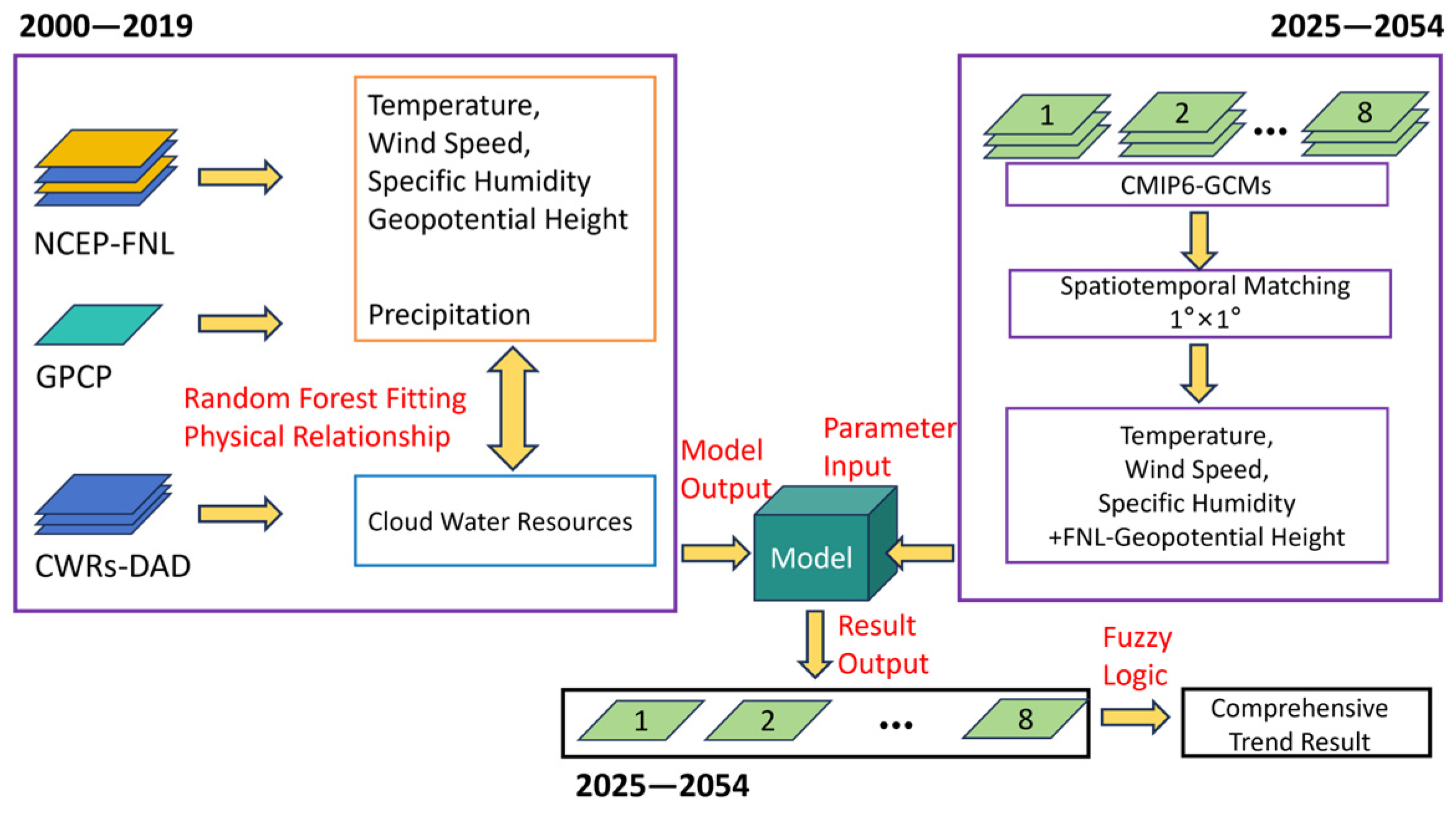
The random forest model can effectively capture the physical relationship between basic atmospheric variables (such as temperature, specific humidity, wind speed, and wind direction) and cloud water resource estimates (calculated using the balance equation). The proposed combination of random forest and fuzzy logic methods can provide estimates of cloud water resources and their overall trends for the next 30 years in China.

(2)

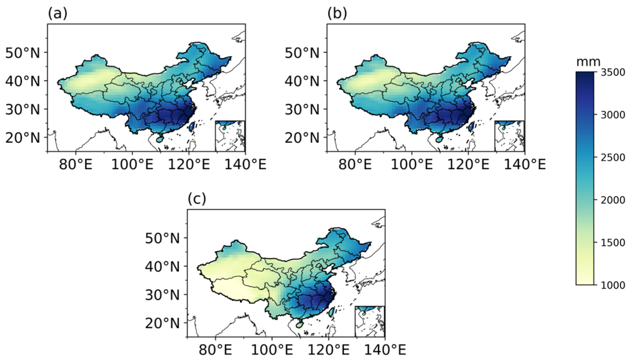
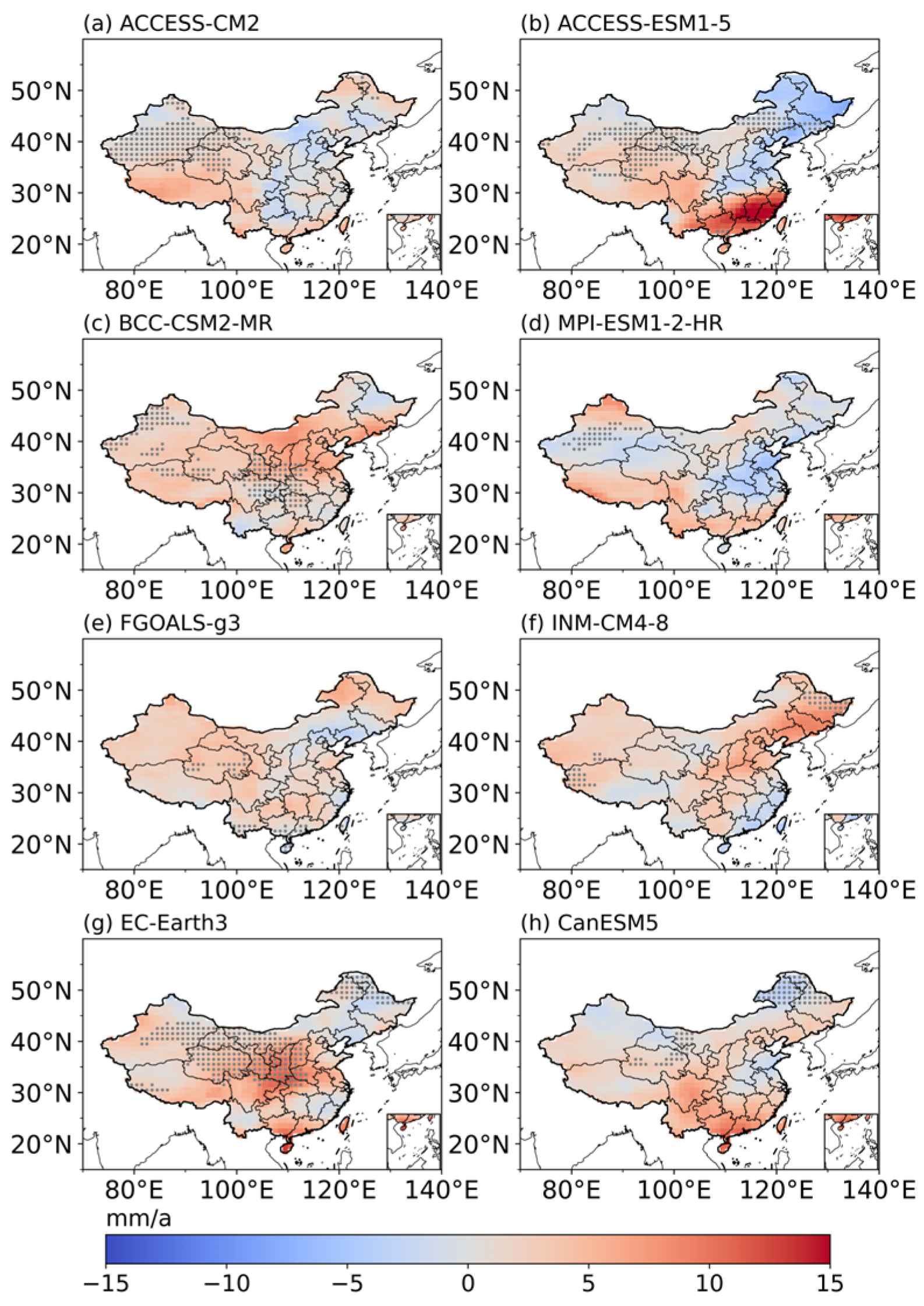
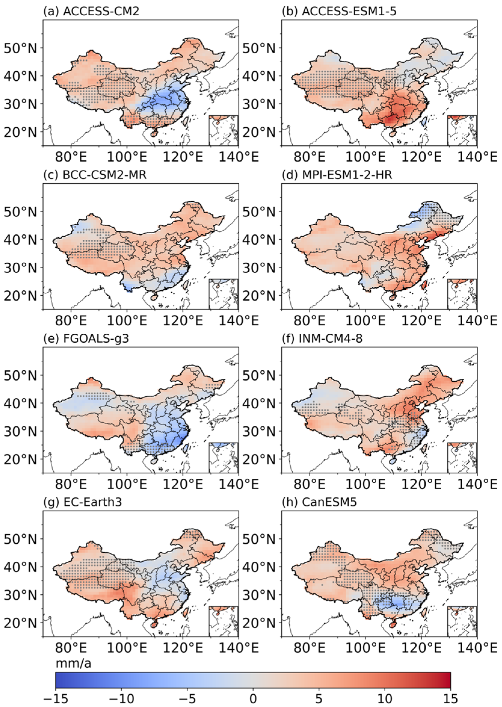
In both future scenarios, the cloud water resources (CWRs) distribution patterns for China from 2025 to 2054 are generally consistent with those from the past period of 2000–2019. The average CWRs in the next 30 years are expected to be higher than in the past, particularly under the high emission scenario. The comprehensive trend of change derived through fuzzy logic inference indicates that the areas of increased CWRs in China over the next 30 years are concentrated in the Tibetan Plateau and the northwest region. Under the high emission scenario, there is a potential for the areas of increased CWRs to expand towards the north.

The above results can provide a reference for weather modification and the development and utilization of cloud water resources in China. By combining regional artificial rainfall needs, it is possible to leverage the control and management capabilities of atmospheric water resources. This is particularly significant for ecological restoration in northwest China, drought resistance in agriculture in the North China and Northeast regions, and ensuring water storage for reservoirs to guarantee water supply for residents in central regions.

References

1. Cai, M. Cloud Water Resource and Precipitation Efficiency Evaluation over China. Ph.D. Thesis, Nanjing University of Information Science and Technology, Nanjing, China, 2013. (In Chinese). [Google Scholar]
2. Benton, G.S.; Estoque, M.A. Water-Vapor Transfer over The North American Continent. J. Meteorol. 1954, 11, 462–477. [Google Scholar] [CrossRef]
3. Lu, Y.; Gao, G. Characteristics of mean water vapor content and water balance in Chinese atmosphere. Acta Meteorol. Sin. 1984, 42, 301–310. (In Chinese) [Google Scholar]
4. Greenwald, T.J.; Stephens, G.L.; Christopher, S.A.; Vonder Harr, T.H. Observations of the Global Characteristics and Regional Radiative Effects of Marine Cloud Liquid Water. J. Clim. 1995, 8, 2928–2946. [Google Scholar] [CrossRef]
5. Li, X.; Guo, X.; Zhu, J. Climatic distribution features and trends of cloud water resources over China. Chin. J. Atmos. Sci. 2008, 32, 1094–1106. (In Chinese) [Google Scholar]
6. He, X.; Song, M.; Zhou, Z. Temporal and spatial characteristics of water vapor and cloud water over the Qinghai-Xizang Plateau in summer. Plateau Meteorol. 2020, 39, 1339–1347. (In Chinese) [Google Scholar] [CrossRef]
7. Zhang, H.; Shi, M.; Wu, H.; Qi, D.; Quan, C. Cloud water resources assessment in Qinghai province based on ERA-Interim reanalysis data. J. Arid Meteorol. 2021, 39, 569–576. (In Chinese) [Google Scholar] [CrossRef]
8. Li, G.; Yan, F.; Ao, J.; Mao, Z. Temporal and spatial characteristics of cloud water resources in Hainan island over the past 30 years. J. Trop. Biol. 2022, 13, 331–338. (In Chinese) [Google Scholar] [CrossRef]
9. Zhou, Y.; Cai, M.; Tan, C.; Mao, J.; Hu, Z. Quantifying the Cloud Water Resource: Basic Concepts and Characteristics. J. Meteorol. Res. 2020, 34, 1242–1255. [Google Scholar] [CrossRef]
10. Cai, M.; Zhou, Y.; Liu, J.; Tan, C.; Tang, Y.; Ma, Q.; Li, Q.; Mao, J.; Hu, Z. Quantifying the Cloud Water Resource: Methods Based on Observational Diagnosis and Cloud Model Simulation. J. Meteorol. Res. 2020, 34, 1256–1270. [Google Scholar] [CrossRef]
11. Tan, C.; Cai, M.; Zhou, Y.; Liu, W.; Hu, Z. Cloud Water Resource in North China in 2017 Simulated by the CMA-CPEFS Cloud Resolving Model: Validation and Quantification. J. Meteorol. Res. 2022, 36, 520–538. [Google Scholar] [CrossRef]
12. Cheng, J.; You, Q.; Zhou, Y.; Cai, M.; Pepin, N.; Chen, D.; AghaKouchak, A.; Kang, S.; Li, M. Increasing cloud water resource in a warming world. Environ. Res. Lett. 2021, 16, 124067. [Google Scholar] [CrossRef]
13. Cai, M.; Zhou, Y.; Liu, J.; Tang, Y.; Zhao, J.; Ou, J. Diagnostic Quantification of the Cloud Water Resource in China during 2000–2019. J. Meteorol. Res. 2022, 36, 292–310. [Google Scholar] [CrossRef]
14. Cheng, J.; You, Q.; Cai, M.; Sun, J.; Zhou, Y. Cloud Water Resource over the Asian water tower in recent decades. Atmos. Res. 2022, 269, 106038. [Google Scholar] [CrossRef]
15. Yu, J.; Cai, M.; Zhou, Y.; Zhao, J. Spatiotemporal Characteristics of Cloud Water Resources in Northwest China from 2000 to 2019. Acta Meteorol. Sin. 2024, 82, 476–489. (In Chinese) [Google Scholar] [CrossRef]
16. He, X.; Chaney, N.; Schleiss, M.; Sheffield, J. Spatial downscaling of precipitation using adaptable random forests. Water Resour. Res. 2016, 52, 8217–8237. [Google Scholar] [CrossRef]
17. Gleick, P.H. Climate change, hydrology, and water resources. Rev. Geophys. 1989, 27, 329–344. [Google Scholar] [CrossRef]
18. Gonzalez, P.; Neilson, R.P.; Lenihan, J.M.; Drapek, R.J. Global patterns in the vulnerability of ecosystems to vegetation shifts due to climate change. Glob. Ecol. Biogeogr. 2010, 19, 755–768. [Google Scholar] [CrossRef]
19. Guo, S.; Guo, J.; Hou, Y.; Xiong, L.; Hong, X. Prediction of future runoff change based on Budyko hypothesis in Yangtze River Basin. Adv. Water Sci. 2015, 26, 151–160. (In Chinese) [Google Scholar] [CrossRef]
20. Song, Z.; Xia, J.; She, D.; Li, L.; Hu, C.; Hong, S. Assessment of meteorological drought change in the 21st century based on CMIP6 multi-model ensemble projections over mainland China. J. Hydrol. 2021, 601, 126643. [Google Scholar] [CrossRef]
21. Zhou, T.; Chen, Z.; Chen, X.; Zuo, M.; Jiang, J.; Hu, S. Interpreting IPCC AR6: Future global climate based on projection under scenarios and on near-term information. Clim. Change Res. 2021, 17, 652–663. (In Chinese) [Google Scholar] [CrossRef]
22. Jiang, J.; Zhou, T.; Chen, X.; Zhang, L. Future changes in precipitation over Central Asia based on CMIP6 projections. Environ. Res. Lett. 2020, 15, 054009. [Google Scholar] [CrossRef]
23. Guo, H.; Bao, A.; Chen, T.; Zheng, G.; Wang, Y.; Jiang, L.; De Maeyer, P. Assessment of CMIP6 in simulating precipitation over arid Central Asia. Atmos. Res. 2021, 252, 105451. [Google Scholar] [CrossRef]
24. Zhang, S.; Hu, Y.; Li, Z. Recent Changes and Future Projection of Precipitation in Northwest China. Clim. Change Res. 2022, 18, 683–694. (In Chinese) [Google Scholar] [CrossRef]
25. Wang, Z.; Zhang, Q.; Sun, S.; Wang, P. Interdecadal Variation of the Number of Days with Drought in China Based on the Standardized Precipitation Evapotranspiration Index (SPEI). J. Clim. 2022, 35, 2003–2018. [Google Scholar] [CrossRef]
26. Xu, C.; Zhao, T.; Zhang, J.; Tao, L. Effects of Human Activities and Natural Forcings on Multiscale Changes of Global Land Surface Air Temperature by CMIP6 Models. Chin. J. Geophsics 2024, 67, 477–491. [Google Scholar] [CrossRef]
27. Zhao, T.; Chen, L.; Ma, Z. Simulation of historical and projected climate change in arid and semiarid areas by CMIP5 models. Chin. Sci. Bull. 2014, 59, 412–429. [Google Scholar] [CrossRef]
28. Zhao, T.; Dai, A. Uncertainties in historical changes and future projections of drought. Part II: Model-simulated historical and future drought changes. Clim. Change 2017, 144, 535–548. [Google Scholar] [CrossRef]
29. Guan, Y.; Gu, X.; Slater, L.J.; Li, X.; Li, J.; Wang, L.; Tang, X.; Kong, D.; Zhang, X. Human-induced intensification of terrestrial water cycle in dry regions of the globe. NPJ Clim. Atmos. Sci. 2024, 7, 45. [Google Scholar] [CrossRef]
30. Tahara, R.; Hiraga, Y.; Kazama, S. Climate change effects on the localized heavy rainfall event in northern Japan in 2022: Uncertainties in a pseudo-global warming approach. Atmos. Res. 2025, 314, 107780. [Google Scholar] [CrossRef]
31. Wang, H.; Su, W. Evaluating and understanding top of the atmosphere cloud radiative effects in Intergovernmental Panel on Climate Change (IPCC) Fifth Assessment Report (AR5) Coupled Model Intercomparison Project Phase 5 (CMIP5) models using satellite observations. J. Geophys. Res. Atmos. 2013, 118, 683–699. [Google Scholar] [CrossRef]
32. Liu, M. Research on the Change Characteristics and Uncertainty Constraint Methods of East Asian Cloud Feedback Under Future Emission Scenarios. Master’s Thesis, Chinese Academy of Meteorological Sciences, Beijing, China, 2023. (In Chinese). [Google Scholar]
33. Cesana, G.; Chepfer, H. How well do climate models simulate cloud vertical structure? A comparison between CALIPSO-GOCCP satellite observations and CMIP5 models. Geophys. Res. Lett. 2012, 39, 2012GL053153. [Google Scholar] [CrossRef]
34. Schlund, M.; Lauer, A.; Gentine, P.; Sherwood, S.C.; Eyring, V. Emergent constraints on equilibrium climate sensitivity in CMIP5: Do they hold for CMIP6? Earth Syst. Dyn. 2020, 11, 1233–1258. [Google Scholar] [CrossRef]
35. Li, L.; Guo, Z. Short Commentary on CMIP6 Cloud Feedback Model Intercomparison Project(CFMIP). Clim. Change Res. 2019, 15, 465–468. (In Chinese) [Google Scholar] [CrossRef]
36. National Centers for Environmental Prediction/National Weather Service/NOAA/U.S. Department of Commerce. NCEP FNL Operational Model Global Tropospheric Analyses, continuing from July 1999. Research Data Archive at the National Center for Atmospheric Research, Computational and Information Systems Laboratory. 2000. Available online: https://rda.ucar.edu/datasets/d083002/ (accessed on 15 July 2023).
37. Adler, R.; Wang, J.; Sapiano, M.; Huffman, G.; Bolvin, D.; Nelkin, E.; NOAA, C. Global Precipitation Climatology Project (GPCP) Climate Data Record (CDR), Version 1.3 (Daily). Available online: https://www.ncei.noaa.gov/data/global-precipitation-climatology-project-gpcp-daily/access/ (accessed on 21 March 2024).
38. Huffman, G.J.; Adler, R.F.; Morrissey, M.M.; Bolvin, D.T.; Curtis, S.; Joyce, R.; McGavock, B.; Susskind, J. Global Precipitation at One-Degree Daily Resolution from Multisatellite Observations. J. Hydrometeorol. 2001, 2, 36–50. [Google Scholar] [CrossRef]
39. Cai, M.; Zhou, Y.; Ou, J.; Liu, J.; Cai, Z. Study on Diagnosing Three Dimensional Cloud Region. Plateau Meteorol. 2015, 34, 1330–1344. (In Chinese) [Google Scholar] [CrossRef]
40. Zhou, Q.; Zhang, Y.; Li, B.; Li, L.; Feng, J.; Jia, S.; Lv, S.; Tao, F.; Guo, J. Cloud-base and cloud-top heights determined from a ground-based cloud radar in Beijing, China. Atmos. Environ. 2019, 201, 381–390. [Google Scholar] [CrossRef]
41. Zhang, L.; Chen, X.; Xin, X. Short Commentary on CMIP6 Scenario Model Intercomparison Project (ScenarioMIP). Clim. Change Res. 2019, 15, 519–525. (In Chinese) [Google Scholar] [CrossRef]
42. Ho, T. Random decision forests. In Proceedings of the 3rd International Conference on Document Analysis and Recognition, Montreal, QC, Canada, 14–16 August 1995; 1995; Volume 1, pp. 278–282. [Google Scholar] [CrossRef]
43. Breiman, L. Random Forests. Mach. Learn. 2001, 45, 5–32. [Google Scholar] [CrossRef]
44. Han, J.; Liu, Y.; Sun, X. A scalable random forest algorithm based on MapReduce. In Proceedings of the 2013 IEEE 4th International Conference on Software Engineering and Service Science, Beijing, China, 23 May 2013; pp. 849–852. [Google Scholar] [CrossRef]
45. Guo, F.; Ma, X.; Wang, T.; Chen, C. An Approach to The Hydrometeors Classification for Thunderclouds Based on the X-band Dual-polarization Doppler Weather Radar. Acta Meteorol. Sin. 2014, 72, 1231–1244. (In Chinese) [Google Scholar] [CrossRef]
46. Liu, H.; Chandrasekar, V. Classification of Hydrometeors Based on Polarimetric Radar Measurements: Development of Fuzzy Logic and Neuro-Fuzzy Systems, and In Situ Verification. J. Atmos. Ocean. Technol. 2000, 17, 140–164. [Google Scholar] [CrossRef]
47. Lim, S.; Cifelli, R.; Chandrasekar, V.; Matrosov, S.Y. Precipitation Classification and Quantification Using X-Band Dual-Polarization Weather Radar: Application in the Hydrometeorology Testbed. J. Atmos. Ocean. Technol. 2013, 30, 2108–2120. [Google Scholar] [CrossRef]
48. Wu, C.; Liu, L.; Wei, M.; Xi, B.; Yu, M. Statistics-based optimization of the polarimetric radar hydrometeor classification algorithm and its application for a squall line in South China. Adv. Atmos. Sci. 2018, 35, 296–316. [Google Scholar] [CrossRef]
49. Weng, Y.; Cai, W.; Wang, C. The application and future directions of the Shared Socioeconomic Pathways (SSPs). Clim. Change Res. 2020, 16, 215–222. (In Chinese) [Google Scholar] [CrossRef]
50. Hu, S.; Zhou, T.; Wu, B. Accelerated warming of High Mountain Asia predicted at multiple years ahead. Sci. Bull. 2025, 70, 419–428. [Google Scholar] [CrossRef] [PubMed]
51. Ma, Q.; You, Q.; Ma, Y.; Cao, Y.; Zhang, J.; Niu, M.; Zhang, Y. Changes in cloud amount over the Tibetan Plateau and impacts of large-scale circulation. Atmos. Res. 2021, 249, 105332. [Google Scholar] [CrossRef]
52. Yan, H.; Huang, J.; He, Y.; Liu, Y.; Li, J. Atmospheric Water Vapor Budget and Its Long-Term Trend Over the Tibetan Plateau. J. Geophys. Res. Atmos. 2020, 123, e2020JD033297. [Google Scholar] [CrossRef]
53. Zhang, J.; Jing, L.; Wang, S. Spatial and Temporal Variations of Cloud Parameters over the Qinghai-Xizang Plateau during the Past Two Decades. Plateau Meteorol. 2023, 42, 1107–1118. (In Chinese) [Google Scholar] [CrossRef]
54. Zhang, Q.; Yang, J.; Duan, X.; Ma, P.; Lu, G.; Zhu, B.; Liu, X.; Yue, P.; Wang, Y.; Liu, W. The eastward expansion of the climate humidification trend in Northwest China and the synergistic influences on the circulation mechanism. Clim. Dyn. 2022, 59, 2481–2497. [Google Scholar] [CrossRef]
Figure 1. Feature importance corresponding to feature parameters. ps denotes precipitation, ua and va represent the horizontal and vertical wind fields respectively, tm indicates atmospheric temperature, tm_surf stands for surface temperature, and q represents specific humidity.
Earth 06 00031 g001
Figure 2. Flowchart of the methods.
Earth 06 00031 g002
Figure 3. Membership function graphs for trend value (a) and p-value (b).
Earth 06 00031 g003
Figure 4. 2D histograms of model predicted values and GT values for the test set: (a). statistical regression model, (b). neural network model, (c). random forest model. Note: The red dashed line represents the 45 degree diagonal.
Earth 06 00031 g004
Figure 5. Daily variation curves of CWRs (grid-averaged) for China in 2005: model estimates (blue) and GT values (red), unit: mm.
Earth 06 00031 g005
Figure 6. CWRs distribution for China on 10 April 2005 (Row 1) and 9 June 2005 (Row 2): ((a,c) are GT Values, (b,d) are model estimates).
Earth 06 00031 g006
Figure 7. Interannual variation curves of cloud water resources (CWRs-Mean) after daily and grid-averaged calculations: (a). under the SSP2-4.5 scenario, (b). under the SSP5-8.5 scenario).
Earth 06 00031 g007
Figure 8. CWRs climate state distribution under SSP2-4.5 for eight climate models: (a). ACCESS-CM2, (b). ACCESS-ESM1-5, (c). BCC-CSM2-MR, (d). MPI-ESM1-2-HR, (e). FGOALS-g3, (f). INM-CM4-8, (g). EC-Earth3. (h). CanESM5.
Earth 06 00031 g008
Figure 9. CWRs climate state distribution under SSP5-8.5 for eight climate models: (a). ACCESS-CM2, (b). ACCESS-ESM1-5, (c). BCC-CSM2-MR, (d). MPI-ESM1-2-HR, (e). FGOALS-g3, (f). INM-CM4-8, (g). EC-Earth3. (h). CanESM5.
Earth 06 00031 g009
Figure 10. Multi-model distribution average results: (a). average results under SSP2-4.5, (b). average results under SSP5-8.5, (c). 20-year (2000–2019) annual average distribution of CWRs in China.
Earth 06 00031 g010
Figure 11. Distribution of CWRs trend change under SSP2-4.5 for eight climate models: (a). ACCESS-CM2, (b). ACCESS-ESM1-5, (c). BCC-CSM2-MR, (d). MPI-ESM1-2-HR, (e). FGOALS-g3, (f). INM-CM4-8, (g). EC-Earth3. (h). CanESM5. Points indicate significant results based on α = 0.05 significance test.
Earth 06 00031 g011
Figure 12. Distribution of CWRs trend change under SSP5-8.5 for eight climate models: (a). ACCESS-CM2, (b). ACCESS-ESM1-5, (c). BCC-CSM2-MR, (d). MPI-ESM1-2-HR, (e). FGOALS-g3, (f). INM-CM4-8, (g). EC-Earth3. (h). CanESM5. Points indicate significant results based on α = 0.05 significance test.
Earth 06 00031 g012
Figure 13. CWRs trend distributions: (a). fuzzy logic inference results under SSP2-4.5, (b). fuzzy logic inference results under SSP5-8.5, (c). CWRs trend for 2000–2019 (points indicate significant results based on α = 0.05 significance test).
Earth 06 00031 g013
Figure 14. Histogram of proportions for different CWRs ranges.
Earth 06 00031 g014
Figure 15. Taylor diagrams of CMIP6 model simulations for surface temperature and precipitation: (a). annual daily average temperature, (b). annual daily average precipitation. Note: The green dashed line indicates the root mean square error (RMSE), the blue dashed line indicates the correlation coefficient, and the black dashed line indicates the standard deviation.
Earth 06 00031 g015