Abstract
This paper addresses the problem of mapping land cover types in Senegal and recognition of vegetation systems in the Saloum River Delta on the satellite images. Multi-seasonal landscape dynamics were analyzed using Landsat 8-9 OLI/TIRS images from 2015 to 2023. Two image classification methods were compared, and their performance was evaluated in the GRASS GIS software (version 8.4.0, creator: GRASS Development Team, original location: Champaign, Illinois, USA, currently multinational project) by means of unsupervised classification using the k-means clustering algorithm and supervised classification using the Support Vector Machine (SVM) algorithm. The land cover types were identified using machine learning (ML)-based analysis of the spectral reflectance of the multispectral images. The results based on the processed multispectral images indicated a decrease in savannas, an increase in croplands and agricultural lands, a decline in forests, and changes to coastal wetlands, including mangroves with high biodiversity. The practical aim is to describe a novel method of creating land cover maps using RS data for each class and to improve accuracy. We accomplish this by calculating the areas occupied by 10 land cover classes within the target area for six consecutive years. Our results indicate that, in comparing the performance of the algorithms, the SVM classification approach increased the accuracy, with 98% of pixels being stable, which shows qualitative improvements in image classification. This paper contributes to the natural resource management and environmental monitoring of Senegal, West Africa, through advanced cartographic methods applied to remote sensing of Earth observation data.
Keywords:
remote sensing; cartography; vegetation; West Africa; satellite image; Landsat; Sahel; climate change; landscape; land cover types PACS:
91.10.Da; 91.10.Jf; 91.10.Sp; 91.10.Xa; 96.25.Vt; 91.10.Fc; 95.40.+s; 95.75.Qr; 95.75.Rs; 42.68.Wt
MSC:
86A30; 86-08; 86A99; 86A04
JEL Classification:
Y91; Q20; Q24; Q23; Q3; Q01; R11; O44; O13; Q5; Q51; Q55; N57; C6; C61
1. Introduction
1.1. Background
Land cover and land use change are widely known as key elements of landscapes. Maps showing classification of land cover types are key data sources for assessment of landscape dynamics and for evaluating environmental trends. Land cover types (or land use types) refer to the physical components of Earth cover that are physically present and visible on the Earth’s surface. Compared to land use types, which are defined as landscape patches used by people, land cover types typically represent natural physical characteristics of the Earth’s surface in terms of structure, patterns, and components. Characteristics and features of land cover types are visible on satellite images recorded from space. Therefore, remote sensing (RS) data, such as satellite images, are widely used for land cover change analysis using classification maps that show spatio-temporal changes in land cover/land use patterns. Hence, land cover maps are the background geoinformation products necessary for analysts and decision makers. The use of land cover maps enables the monitoring of environmental changes and evaluation of risks to sustainable development. Therefore, the use of land cover maps is applicable in diverse research and development sectors such as governments, civil engineering, and industrial planning [1].
In monitoring landscape dynamics, remote sensing (RS) data are widely used and applied in environmental mapping with the aim of detecting identical landscape patterns in a time series of images and analyzing changes using recognition of landscape patches. In this regard, there is a strong need for machine-based, automated geospatial data processing and image analysis that turns the technical values of pixels in the satellite images into information that provides knowledge and insights for environmental experts and planners. The identification and recognition of land cover types becomes possible using the analysis and synthesis of remote sensing data, such as spaceborne images. Environmental studies often use such products for landscape analysis, for example, images of Landsat missions.
Major types of satellite images for effective interpretation of the Earth’s landscapes include Sentinel 2 Data [2,3], NOAA-AVHRR [4,5,6], SPOT [7,8], and Landsat [9,10], and the combinations thereof [11]. For instance, the recent Global Land Cover 2000 map was implemented using the analysis of the Vegetation Sensor on board the SPOT-4 satellite image [12]. Another example of such products is presented by the time series of annual global maps of land cover types derived from the ESA Sentinel 2 imagery at 10 m resolution [13]. The Landsat scenes used for landscape mapping include data acquired from its various sensors, such as the Multispectral Scanner (MSS), the Thematic Mapper (TM), the Enhanced Thematic Mapper Plus (ETM+), and the recent product called the Operational Land Imager and Thermal Infrared Sensor (OLI/TIRS).
Certainly, although diverse images can be used in various combination as data sources for landscape interpretation and environmental mapping, the general approach of RS data processing relies on using the values of spectral reflectance obtained as digital numbers (DNs) of pixels on the image scene [14]. The effects of reflectance and absorption of various land cover types in different wavelengths enable the discrimination of major land cover types in the multispectral images: water, land, forests (with various types of vegetation), urban zones, and desert sands [15]. Such information can be extracted from variations in brightness, primary colors (red, green, blue), hue, saturation, and intensity of light. In experimental studies, these phenomena are utilized to assess land–water borders and distinguish them from other land cover types, leading to an improvement in the recognition of the Earth’s objects [16]. The information provided by the environmental descriptors can be obtained from the analysis of values of pixels recording spectral reflectance of diverse land cover types. In RS, this can be derived from the combination of different bands of the multispectral imagery, e.g., NIR/Red bands for computing the Normalized Difference Vegetation Index (NDVI) and other vegetation indices [17,18,19,20].
1.2. Problem Formulation
One of the challenging problems in identification of land cover types in the satellite images consists of automatic extraction of the reliable features visible in the image scene. This is true especially in terms of highly heterogeneous landscape patches in a complex mosaic of intermittent land cover types [21,22]. In this regard, image processing and analysis for landscape interpretation are fundamental issues in environmental mapping and thematic cartography. Identification of land cover types in the RS data requires diverse image processing techniques, such as classification, clustering, and segmentation. Classifying mixed terrestrial ecoregions typical for Senegal requires advanced methods of image analysis [23]. Senegal’s landscape is distinctive because it consists of a complex blend of diverse, semi-arid landscapes, such as forest–savanna mosaics, which are periodically filled with Sahelian acacia and West Sudanian savannas with diverse tree species, as well as coastal regions with dominant Guinean mangroves [24,25].
The current practice of geographic information system (GIS)-based supervised image processing involves manually marking different features in a landscape, such as regions of interest (ROIs), singular patches, and landscape corridors, because the extraction of features from processed images is difficult [26]. The human factor in landscape assessment involves some concerns about the repeatability and reliability, which suggest the need for the development of automatic methods for image interpretation and object recognition [27,28,29]. Manual interpretation of land cover types can lead to the misclassification of pixels in the images, which might result in misinterpretation of the selected landscape patches. As mentioned earlier, implementing quantitative data interpretation for prediction and analysis is challenging in African countries where fieldwork data are limited [30]. Therefore, RS-based vegetation mapping and agricultural landscape monitoring are vitally dependent on using satellite data processed with a high level of automation [31,32].
Effective image analysis relies heavily on the type of classifier and the algorithms used for data handling [33]. Another important factor is the quality of imagery for the evaluated region of interest (ROI) in the study area, which includes minimal cloudiness and haze, correct time of image capture and coverage. Finally, image analysis is based on the methodology and approaches used in RS, including data acquisition, preprocessing, description, recognition, classification, segmentation, interpretation, and accuracy analysis. The development of computer-based programming methods has led to the growth of novel image processing methods, which are the primary factors in effectiveness [34,35,36,37,38]. Development of the advanced tools of image processing and related cartographic tasks has resulted in many approaches to utilizing effective methods for automation [39,40,41,42,43,44]. One of these methods is the machine learning (ML)-based Support Vector Machine (SVM) algorithm used for image analysis and synthesis for interpretation of vegetation patterns [45,46,47,48].
In this respect, the research questions formulated in this study are as follows: (1) Can the Support Vector Machine (SVM) ML-based land cover detection method be used with GIS for satellite image analysis? (2) How can the SVM algorithm of ML be employed in geoinformation extracting tasks using scripts? (3) What is the workflow for RS data processing for an effective chain of data handling to perform the necessary tasks during SVM-based image classification? Answering these questions enables us to evaluate the effectiveness of SVM as one of the most powerful ML applications in cartographic tasks and RS data analysis.
1.3. Related Work
Many reports have recently been published illustrating land cover changes in Senegal [49,50,51], effects of climate change on landscape variability and vegetation communities [52,53,54], environmental dynamics, and sustainability [55]. Nevertheless, these approaches do not take into account the benefits of programming scripts for satellite image processing. At the same time, using ML methods increases the automation of mapping and the speed of data processing, ensuring the accuracy and objectivity of land cover classification. Indeed, image processing using ML methods such as SVM partitions the image into structured land patches using automatic analysis of spectral reflectance of the pixels. The obtained values of pixels are then assigned into various classes using principles of machine-based vision and pattern recognition. Through this approach, it is easy to visualize and estimate changes in land cover types using images from different years as part of a time series analysis. Additionally, it overcomes the problems with conventional software programs used for image processing, which may include drawbacks in data processing.
A drought period in Africa in the 1970s and 1980s resulted in climate changes that include such consequences as decreased rainfall and precipitation, raised temperatures, and increased evaporation [56,57]. These climate-related processes triggered land cover changes in natural vegetation patterns of Sahel ecoregions that affected cultivated areas and croplands, increased spots of bare soil, and led to changes in surface water [58,59]. To this point, one of the priorities of image processing methods for environmental landscape analysis is to support land cover monitoring through the interpretation of land cover types using time series analysis. Regular monitoring of the Earth’s landscapes enables us to detect environmental changes, land and soil degradation, and variations in vegetation cover [60]. Another essential application of image analysis is monitoring coastal zones to evaluate hydrological changes, to evaluate the extent of river flooding in the delta, to detect soil erosion [61,62], and to monitor the degradation of mangroves and coastal ecosystems [63,64].
1.4. Objective and Motivation
Inspired by the existing examples of the ML methods used to analyze multispectral satellite images in environmental applications, this study integrates advanced cartographic scripting methods with applied techniques of SVM image processing for monitoring landscapes in Senegal; see Figure 1.
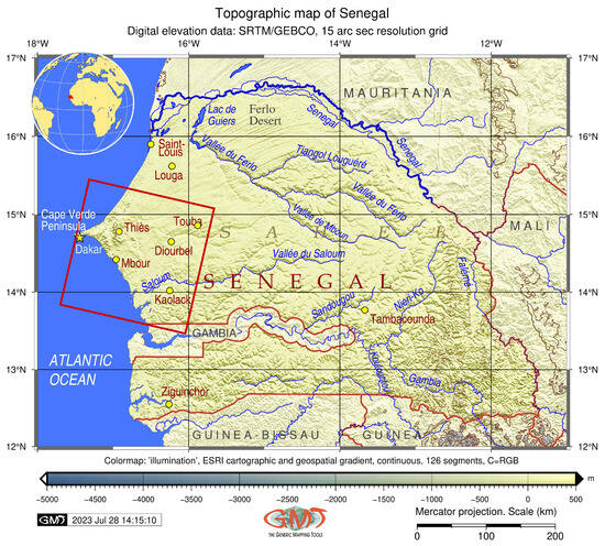
Figure 1.
Study area with segments of the Landsat images shown on a topographic map of Senegal. Software: GMT. Map source: Author.
The environmental analysis was performed using a series of satellite images evaluated for the period from 2015 to 2023. To this end, we explore the classification approach of SVM, which was employed for RS data processing by the scripting techniques of the Geographic Resources Analysis Support System (GRASS) GIS. The SVM classifier is applied as a widely implemented supervised learning approach. Other advanced deep learning (DL) methods that have been developed recently include such methods as autoencoders, a special type of neural network that operates with dimensional latent representation, and vision transformers, which differentially weigh the significance of each part of the image. Nevertheless, SVM is still a sufficient and effective approach for many remote sensing (RS) and GIS tasks. Given the availability of SVM in GRASS GIS, this method was employed for the image classification.
The main goal of this study is to map and evaluate changes in diverse land cover types in West Senegal, which include both inner regions and coastal mangrove forests in the delta of the Saloum River; see Figure 1. To achieve this goal, the practical objective is to classify land cover types in the coastal region of West Senegal using a series of Landsat 8-9 OLI/TIRS multispectral satellite images processed using ML methods, including SVM as an advanced method of automated image classification. Contrary to the existing GIS, the programming approach to satellite image processing has a high automation in data handling. Additionally, it is a very fast and robust approach for classifying and comparing satellite images. This is achieved by a combination of the embedded GRASS GIS modules is used separately for computing vegetation indices and plotting the classification maps.
According to recent studies, mangrove habitats are drastically disappearing. This is because these ecosystems are being impacted by anthropogenic activity, climate change, and local effects of salinity in the soil [65,66]. By evaluating gains and losses in landscape patches, RS data can be spatially analyzed to understand the dynamics of these distinct wetland ecosystems. Our comprehension of the changes in Senegalese landscapes is aided by satellite image analysis, which shows how these landscapes respond to the effects of West Africa’s changing climate, including rising temperatures, evaporation, and falling precipitation.
The goal of using the GRASS GIS scripts for RS data analysis is to quantitatively evaluate changes in land cover types in Senegal as a result of climate fluctuations during a recent eight-year period. The approach to achieve this goal is based on using automated unsupervised classification and supervised classification using the ML method of SVM. In this way, the maximal likelihood and SVM classification algorithms present an effective means by which the Landsat scenes can be processed automatically. The RS data obtained from the United States Geological Survey (USGS) repository were used for environmental analysis and monitoring to evaluate and visualize variations in landscape patches. This analysis is technically based on the ML-based estimation of spectral reflectance on the satellite images, which supports environmental monitoring of the West African landscapes responding to climate and anthropogenic effects.
The main purpose of this paper is to provide an advanced approach using ML to RS data analysis and processing. Such an approach can evaluate the nonlinear behavior of the landscapes in West Africa over time, which indicates the development of climate settings and the related response of vegetation patterns. To this end, we propose a script-based classification and image enhancement technique using GRASS GIS software to analyze land cover changes in the coastal region of West Senegal. This technique aims to address the main challenges associated with traditional image processing, such as structured noise in the classified scenes, poor quality of the images, the misinterpretation of pixels, and the low speed of data handling.
The ML-based image analysis is based on using the RS data, which serve as a cartographic basis to support optimized decisions made by environmental policy makers and planners. Satellite images processed by the machine-based methods allow for the identification of vulnerable landscapes and enable the monitoring of degraded lands in Senegal. In order to do this, a series of the multispectral satellite images from Landsat with recent OLI/TIRS sensors taken on different years was processed with various modules of GRASS GIS. This time series data analysis enabled us to perform an environmental analysis for monitoring landscape dynamics in Senegal.
Importantly, the study presented here is not intended to suggest that scripting methods replace the role of conventional GIS. In contrast, the programming codes supplement the traditional cartographic methods used in the RS software. However, the integration of a scripting workflow with image analysis and cartographic tasks provides an effective approach by which the analysis of land cover changes can be visualized in an automatic way. In light of this, the main contributions of this paper are as follows:
- A combination of the GRASS GIS modules ‘i.group’, ‘i.maxlik’, and ‘i.cluster’ are proposed for the unsupervised image classification. The land cover types are classified based on the difference in spectral reflectance of the pixels in each of the images.
- A set of GRASS GIS modules, including ‘r.learn.predict’, ‘r.learn.train’, and ‘r.random’, is used for supervised ML-based image classification using an SVM modeling algorithm.
- The land cover types in coastal Senegal are defined as groups of pixels according to the structural similarity between the landscape patches. Orientation, location, and frequency of mangrove fields in the Saloum River Delta are estimated from the analysis of landscape patches in the coastal area.
- To balance the robustness and accuracy, a coarse-to-fine strategy is proposed using the interpretation of landscape patches according to the FAO scheme of land cover types. The data for the whole country were downscaled to the ROI of the selected study area, with images covering the region of Cape Verde Peninsula and the surrounding territories.
- The proposed image processing and ML-based classification algorithms utilizing the SVM techniques of GRASS GIS outperform the existing traditional software with graphical user interface (GUI) approaches in terms of repeatability of scripts and automation through computer vision. This methodological workflow is useful for future similar studies of land cover type analysis in Senegal or surrounding areas of West Africa.
2. Materials and Methods
To increase the speed and accuracy of image processing, the GRASS GIS software was applied for advanced image processing due to its extended functionalities [67]. Generic Mapping Tools (GMT) Version 6 [68] was used as a cartographic tool for topography, and RS tasks are based on scripting techniques. The main advantages of scripts include their high speed of data processing and repeatability [69,70,71].
2.1. Data
We use six Landsat 8-9 OLI/TIRS images for evaluation of land cover changes in western Senegal from 2015 to 2023. Major metadata are summarized in Table 1.

Table 1.
Identifiers (IDs) of the six multispectral Landsat 8-9 OLI/TIRS images.
The images were downloaded from the United States Geological Survey (USGS) EarthExplorer repository; see Figure 2. The data contain scenes taken during the winter period (January/February). The selection of the winter period is explained by the fact that images taken during winter enable us to better detect plant phenology in a semi-arid climate. In contrast, those collected during summer are not suitable for plant detection due to the high level of droughts in the desert areas, especially in the inner regions of the country. Additionally, the images were collected with minimized cloudiness and haze below 10%. Hence, the best quality and suitability of images was in the winter period, during the months of January and February. All Landsat images are multispectral and have a 30 m resolution in visible spectral bands. The images are projected in Universal Transverse Mercator (UTM) Zone 28 for western Senegal. The Landsat images used in this study are presented in Figure 3.
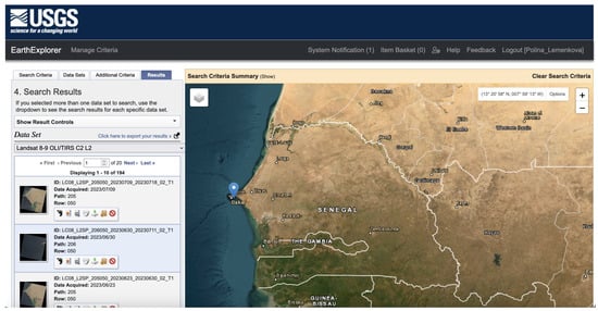
Figure 2.
Data capture of Landsat images from the USGS EarthExplorer repository.
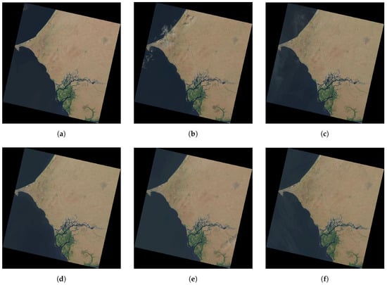
Figure 3.
Landsat images in RGB colors covering the Cape Verde Peninsula region and Saloum River Delta, West Senegal, in February: (a) 2015; (b) 2018; (c) 2020; (d) 2021; (e) 2022; (f) 2023.
It is well-known that the high-resolution commercial satellite images (e.g., SPOT, Pleiades) are expensive due to the expenses related to the launch of the satellite and related operational costs. Therefore, such scenes are not always easily accessible as a data source. Hence, the use of the open source Landsat 8-9 OLI/TIRS is crucial, and the value of these products to environmental monitoring is high. This is especially true for replication of this study in future similar work. The aim of the multispectral Landsat images was to examine the impact of both anthropogenic and climatic factors on the process of land cover change in western Senegal. This was achieved by analyzing and processing the spectral reflectance characteristics of the pixels obtained from the RS data.
The images were selected for different years (2015 to 2023) for comparability. Using RS techniques, the environmental characteristics of the landscapes were evaluated in order to analyze how changes in climate are affecting the types of land cover and, in particular, the distribution of mangroves along the Saloum River Delta. The metadata for the images were evaluated for each scene: four images were selected from the Landsat-8 OLI-TIRS sensor, and two recent scenes were selected from the Landsat-9 OLI-TIRS sensor instruments.
2.2. Methodology
The methodology of this study is based on scripting software for data processing. Technically, we propose a novel mapping method using the SVM algorithm in GRASS GIS for improving the image classification task, and we compare it with the conventional method of unsupervised classification using k-means clustering. Major programming scripts are shown in Appendix B for technical reference. The full codes have been placed in a GitHub repository, including ML techniques of SVM). The advantage of the GRASS GIS approach to RS data processing consists of adjusted modules enabling us to analyze spectral properties of the satellite images. Additionally, the GMT was applied for cartographic mapping. This paper presents a series of scripting experiments that utilize both software applications. Methods of applied programming enabled us to evaluate recent dynamics of land cover types in Senegal.
The advanced script-based cartographic methods of monitoring and mapping land cover types are built on a growing demand for time- and cost-effective approaches in cartographic workflow and RS data analysis. Their use enables us to save time and resources while processing large geospatial datasets using satellite images obtained from open sources. Hence, three major script-based tool sets were used in this study for geospatial data analysis and environmental monitoring in West Africa:
- The GMT script was used for plotting the topography of the country; see Listing A1.
- An R script was used for plotting the methodological flowchart; see Listing A2.
- GRASS GIS scripts were used for image processing; see Listings A3 and A4.
The main idea was to apply a single workflow framework for both the image processing and the cartographic mapping tasks using scripts run from the console. This enabled us to reveal the advantages of the technical performance of automated geospatial data processing. More specifically, using a programming approach that includes various programming suites from the script-based software presents a novel workflow for geospatial data processing. This method demonstrates how adding scripts expedites the process of image analysis and cartographic plotting while also providing an overview of the study methods. As mentioned earlier [72], the automation of the cartographic procedure and the workflow’s repeatability in future research are the primary benefits of scripts. Moreover, scripting enables us to save significant time due to automation. We were able to identify changes in the analysis of landscapes of western Senegal for the assessment of environmental impacts from climate change by using the information obtained from the automated image analysis and interpretation. This was done by evaluating a series of images and analyzing RS data.
The workflow of the data processing and major methodological steps is shown in Figure 4, with the goal of performing image classification and interpretation in order to detect changes in land cover types. The data processing was technically implemented using GRASS GIS software [73] and run on a Mac machine with Apple M1 chip and the MacOS operating system. After preprocessing and data import, the images were grouped to select the necessary multispectral raster bands for image processing. This was performed by the ’i.group’ module of GRASS GIS [74]. Afterwards, the images were clustered using unsupervised classification. This was carried out utilizing the module ’i.cluster’, which automatically assigns pixels into groups according to their spectral reflectance. This method of image processing provided enough data to group the pixels into land cover types and to evaluate the values of pixels in the actual scenes for comparison. The average computation time for image classification and enhancement per Landsat scene is about 2.5 s.
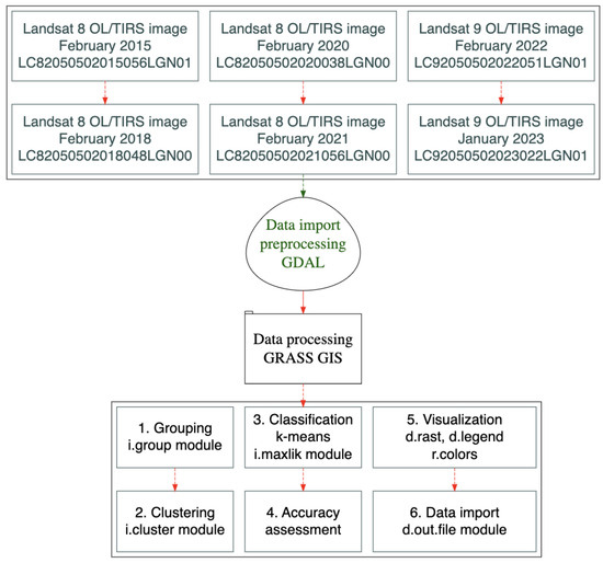
Figure 4.
Workflow scheme illustrating the data and the main methodological steps. Software: R version 4.3.3, library DiagrammeR version 1.0.11. Diagram source: Author.
The matching performance of landscape patches over this period is evaluated using GRASS GIS functionality as a sequence of modules utilized for processing each scene separately using a script. The images were read into the GRASS GIS environment using the ’r.import’ module; the list of the available bands was checked using the ’g.list rast’ command. The extent of the ROI (UTM Zone 28) and the resolution were set to the region of the current image, which was detected automatically along with geospatial data such as coordinates, location, and projection. The false color composites were plotted to distinguish the area of vegetation in the delta of the Saloum River (colored in red shadows), land (colored by beige and light brownish shadows), and water areas (colored black for seawater and navy blue for the Saloum River); see Figure 5.
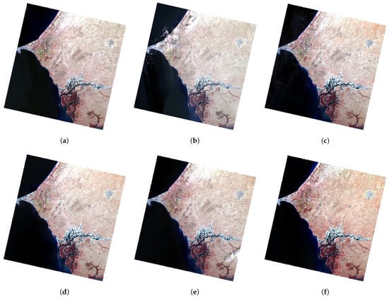
Figure 5.
False color composites of the Landsat 8-9 OLI/TIRS images with vegetation colored red, using a combination of spectral bands 5 (Near Infrared (NIR)), 4 (Red), and 3 (Green) of the Landsat OLI sensor covering the study area in the Cape Verde Peninsula region and Saloum River Delta, West Senegal, using February scenes: (a) 2015; (b) 2018; (c) 2020; (d) 2021; (e) 2022; (f) 2023.
The ML method of satellite image processing involves using the SVM algorithm for data partition and classification. To perform these steps with fixed ML parameters, we utilize the GRASS GIS modules ’r.random’ for generating a training dataset from pixels obtained from the land cover classification, the ’r.learn.train’ module for training a Support Vector Classification (SVC) model, and the ’r.learn.predict’ module, which predicts the pixel’s assignment to the target classes. We represent the image dataset as a time series of scenes from 2015 to 2023 represented as color composites from the multispectral bands of Landsat. We denote the number of estimators as 500 in the model and the number of seed points as 100 pixels, with a total of 1000 evaluated pixels (’npoints’ in the model’s syntax). The training model name is explicitly defined as ’SVC’, i.e., Support Vector Classification, as it is the algorithm embedded in the GRASS GIS software.
The standard requirements for a training dataset in the ML approach that includes the SVM algorithm include a supervised classifier to derive an accurate and precise description of the spectral properties of each land cover type. Therefore, the training data were derived from the previous raster dataset in TIFF format as samples that support vectors through data partition. The target pixels were selected as representative cells located on the edge of the class distribution in feature space. Using GRASS GIS syntax, generating the training pixels from the land cover classification was performed using the following code: ‘r.random input=L_2015_clusters seed=100 npoints=1000 raster=training_pixels’. Here, the number of pixels was selected as 1000 for a larger and more representative dataset, and the seed for training the data was set to 100.
Afterwards, the contrasting regions that have distinguished spectral reflectance values (water, savanna, forest, croplands, and urban spaces) were used for identification of similar classes in the evaluated periods. Then, the land cover classes were identified using the SVM algorithm with the modules ‘r.learn.train’, which trains an SVM model, and ‘r.learn.predict’, which performs prediction of pixels’ association with each of the 10 target land cover classes based on the spectral reflectance of pixels in the images.
3. Results and Discussion
3.1. Interpretation of Key Findings
In this section, the ability of the two algorithms—unsupervised classification by k-means and supervised classification by SVM—to detect land cover changes in the satellite images is evaluated. Specifically, we assessed the dynamics in the distinct habitats of Senegal ranging from arid landscapes with savanna to humid coastal conditions with mangroves. The data for the land cover types in Senegal were visualized in the QGIS software using vector layers in the Environmental Systems Research Institute (ESRI) format; see Figure 6.
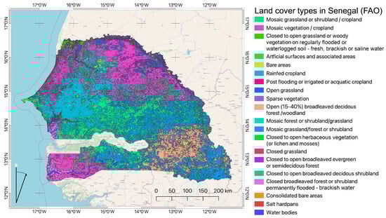
Figure 6.
Land cover types in Senegal according to the FAO classification scheme. Software: QGIS v. 3.22. Map source: Author.
According to the Food and Agriculture Organization (FAO)/United Nations Environment Programme (UNEP) classification scheme, the land cover types in Senegal include 10 major classes. These were adopted for the target extent of the ROI through generalization at the country level using the Land Cover Classification System (LCCS) of FAO/UNEP:
- Mosaic grassland or shrubland/cropland;
- Mosaic vegetation/cropland;
- Mangrove wetlands;
- Rainfed cropland;
- Consolidated bare areas;
- Mosaic grassland/forest or shrubland;
- Closed broadleaved forest or shrubland permanently flooded—brackish water;
- Salt hardpans;
- Post-flooding or irrigated or aquatic cropland;
- Water bodies.
The quantitative estimations of changes in land cover types over the evaluated period (2015 to 2023) are summarized in the tables in Appendix C. They report the computed changes in land cover classes for each processed image. The analysis of these values shows that the northern and southern coastal ecosystems of western Senegal have a relatively small degree of change over the estimated period. In contrast, in the arid north, areas associated with forests and mosaic types of vegetation demonstrate higher magnitudes of change, suggesting a higher level of instability compared to the estuaries in the south. The classification of the land cover types was adapted to the larger extent of the ROI with details for the coastal area, including mangrove forests. The territory of Senegal comprises eight major biological zones with 11 different forms of land use. Of these, major types include the savanna, cultivated lands, forests, and steppes as the dominating types of land cover in the semi-arid zones [75].
A special focus of coastal Senegalese landscapes is mangrove swampland, a crucial habitat in the west of the country. Mangroves provide a source of natural resources [76] and a habitat for wildlife species [77]. At the same time, diverse factors have strongly correlated with mangrove losses. These include climate-related processes such as changes in temperature and precipitation, flooding, and increased salinization of waters, as well as human-related factors such as increases in intensive urbanization [78] and active agriculture practices [79]. Overall, the analysis of land cover types over the coastal area shows the variability in mangroves (bright cyan in Figure 6). Coastal dynamics are explained by high interannual fluctuations in the delta of the Saloum River: the upper tidal zone is flooded during high tide, while during the drought period, it remains drained, with high evaporation resulting in soil salinization.
3.2. Clustering-Based Classification
The overview of Figure 7, on which are overlaid the 2015–2023 Landsat OLI/TIRS time series and the land cover types for each case, shows the diversity of habitats and the intensity of changes detected in the images classified by the k-means algorithm. The analysis of the classified images based on clustering shows a trend in land cover dynamics of the coastal region of Senegal over Dakar and its surroundings.
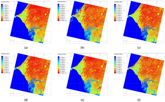
Figure 7.
Classification of the Landsat images from 2020 covering the Cape Verde Peninsula region and the Saloum River Delta, West Senegal: (a) 2015; (b) 2018; (c) 2020; (d) 2021; (e) 2022; (f) 2023.
The results demonstrate that the dominating land cover type of Senegal remains savanna (73%), although the areas covered by savanna showed a slight decrease since 2015. In contrast, the landscapes covered by croplands and agricultural areas expanded to 22%. Furthermore, the decline in the area covered by forests and mangroves is notable. Nevertheless, in general, the dominating land cover types in Senegal remain savannas, woodlands, and forests, covering over 75% of the country, a result aligned with similar studies [24].
The maps of land cover change based on the classified imagery display different spatial patterns. While forest and savanna in the subplots have a significantly higher magnitude of values than the background, this is not the case for the bushland and grasslands, where the difference between the values inside and outside is minimal. The croplands demonstrate moderate changes that indicate the measures taken for sustainable management in Senegal. Overall, landscape heterogeneity can be observed in comparing the processed images. The southern sector of Senegalese vegetation is characterized by the Sudano-Guinean forest savanna and the Guinean forests [80].
The most pronounced variations in land cover types in western Senegal detected on the processed and classified satellite images reflect the relationships and links between changing vegetation and soil characteristics that are subject to climatic factors, moisture level, salinity, and organic matter, as noted earlier [81]. Moreover, the pattern of changes in the agricultural land cover types over time correlate with seasonal fluctuations in the crop–fallow cycle. Agricultural plantations and irrigated lands are distributed in sporadic settlements along the populated and semi-urban areas. Earlier studies also noted [82] that climate variability is the dominant factor that leads to increasing the actual evaporation and, as a result, to land salinization in the basin of the Senegal River.
3.3. Support Vector Machine (SVM)-Based Classification
The SVM-based classification of the dynamics of land cover types in Senegal based on the Landsat OLI/TIRS scenes (2015–2023) resulted in the generation of the thematic maps of land cover types shown in Figure 8, in which the most important classes are identified as follows: the rainfed cropland class is depicted in aquamarine; water areas are shown in blue; mosaic vegetation is colored bright red; and grassland, forest, and shrubland areas are shown in orange. The numerical results obtained for the different images using classification models of GRASS GIS are summarized in Appendix C. Generally, the classification of the Landsat scenes using the SVM algorithm applied to the reflective multispectral bands of the image (channels 1 to 7) provided excellent results for each kernel of the 10 categorized classes.
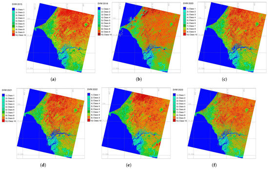
Figure 8.
Results of the Support Vector Machine (SVM)-based classification of the Landsat images covering the Cape Verde Peninsula region and Saloum River Delta, West Senegal: (a) February 2015; (b) February 2018; (c) February 2020; (d) February 2021; (e) February 2022; (f) February 2023.
The aim of the SVM application is to improve the accuracy of recognition of land cover types and to increase the quality of mapping. The feasibility of land cover change analysis depends on the quality of cartographic techniques when processing RS data. Erroneously recognizing trends may arise from the use of land cover regions derived from unadjusted classifiers that exhibit imbalanced misclassification between distinct groups. Therefore, in our work, we used the effective approach of the SVM algorithm proposed by GRASS GIS, which presents a ML approach for image classification. The scripts used for SVM-based image processing are presented in Appendix B.
The detected landscape dynamics evaluated using a time series of the satellite images indicate the cumulative effects of anthropogenic activities and climate change in the semi-arid region of West Africa. This involves such processes as variability of precipitation, increase in temperature, land erosion, and wildfire. These factors control the distribution of croplands, natural vegetation systems, and coastal mangrove colonies in western Senegal. The main triggers for changing types of vegetation and landscape patterns in the Senegalese Sahel include climatic factors and anthropogenic activities, which have resulted in the decline and local extinction of woody species [83].
Among other land cover types, the relics of the Guinean forest are distributed in the northern part of Senegal as a narrow band of landscapes stretching parallel to the Atlantic coast. In the southern and eastern regions off Dakar and around the region of Thiès, there are many species that are abundant in the north of the forest and represented by the scattered trees in the Sudano-Sahelian savanna.
To the east of Dakar, the northern silvopastoral zone of Senegal presents a vast silvopastoral zone characterized around the Ferlo region, which is notable for its extreme aridity, dominated by land cover types of shrubby savanna and steppe vegetation [84]. The enclaves of hygrophilous vegetation surrounding the coastal wetlands are located to the north of Dakar, with mangroves as the dominant land cover type. Additionally, this region includes the occasional groves of the oil palm as spontaneous landscape features of the Guinean forests.
3.4. Accuracy Analysis
Figure 9 shows the results of the accuracy assessment. The correctness of the assignment of pixels to the target classes was evaluated based on the pixel confidence levels with rejection probability values. Using the algorithms embedded in GRASS GIS, six classified Landsat images were evaluated against the probability of the identified pixels being classified into the correct land cover class. In this way, possible misclassification that may arise due to the similar spectral reflectance values in land cover types was assessed. It can be seen that there is a good linear correlation between the contours of the land cover classes and the accuracy of the classification of pixels. The estimation of the values of spectral reflectance indicates a general assignment to a given land cover type. The results are similar for the classified Landsat images processed by means of scripts and correspond to the different land cover types, such as coastal areas, water, savanna, Guinean forests, and agricultural lands.
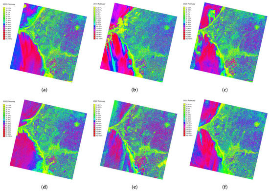
Figure 9.
Accuracy evaluated based on the pixel confidence levels with rejection probability values for the Landsat images covering the Cape Verde Peninsula region and Saloum River Delta, West Senegal: (a) 2015; (b) 2018; (c) 2020; (d) 2021; (e) 2022;(f) 2023.
3.5. Implications and Discussion
Land cover types in Senegal present fluctuations in vegetation patterns as a result of long-term landscape evolution in West Africa [85,86,87,88]. The cumulative effects of climate, environmental, and anthropogenic factors led to a decrease in mangrove colonies, which decline in high-salinity waters [89]. This is also supported by previous studies that report the retreat of the mangrove in the advance of the tannes [90]. At the same time, the trend in rainfall recovery in West Senegal since the 1990s [65] has resulted in the rehabilitation of mangroves, which restored their colonies accordingly, as also visible on the images. This corresponds with the results of the existing reports on the location and distribution of Rhizophora mangle and Avicennia germinans mangrove species in western Senegal [91,92]. Earlier works also noted the increase in mangrove trees in the estuaries of Senegal [93]. In addition to the coastal ecosystems, the areas occupied by crop production follow the same trend in changes, possibly due to vegetation removal associated with plot preparation on agricultural land.
Human-induced activities such as agricultural, demographic, and socioeconomic changes have affected the environmental settings and habitats of Senegal. Although the human impacts on the region were negligible for decades due to the relatively low population density of Senegal, recently, a natural increase in the population has accelerated the exploitation of natural and mineral resources. As a result, this has triggered land degradation in the coastal areas. Consequently, select landscapes of Senegal are subject to the deterioration of valuable habitats, fragmentation of patches, and land cover changes. Major human-induced factors in Senegal are related to dynamic agribusiness in terms of agricultural commodities, which increases the areas of irrigated vegetation and croplands [94]. Although such activities are vital for supporting the local population, the environmental consequences on Senegalese landscapes include changed land cover types. Additionally, land degradation in the savanna landscapes correlates with trends in land cover changes and a significant decrease in woodlands [95].
To summarize, this paper reports the results obtained from experimental investigations into land cover types in Senegal analyzed using a ML approach and the SVM algorithm, compared and evaluated against the traditional unsupervised classification method of k-means clustering. The performance of SVM demonstrated reliable results in image processing, outperforming clustering in terms of accuracy and speed of data processing. To this end, a time series of Landsat scenes was processed using GRASS GIS software. The image processing was designed using a set of modules processed by scripts for automation. Interactive processing and scripts adjusted for each scene provided an effective way to process satellite images in workflow chain. Such automation enabled us to represent complex interactions within the landscapes in a short-term perspective by accurate ML-based mapping using a comparison of the SVM and k-means methods. In this way, this study has presented an advanced data-driven method of image analysis for automatically detecting changes in land cover types in a selected ROI of Senegal.
4. Conclusions
Mapping land cover types, discriminating mangroves, and monitoring savanna ecosystems are essential for proper land management in Senegal. In this study, the potential for employing the SVM algorithm classifier in conjunction with Landsat OLI/TIRS multispectral satellite images was evaluated to map areas of land cover in the environment of Senegal. In an effort to drive research in this field, this paper proposed a series of image classification experiments using the GRASS GIS scripting approach, which served as a means of ranking landscapes. Using processed satellite images, land cover development was evaluated in the condition of the unstable environmental setting of western Senegal, which has been affected by climate change and human activities. The practical aim was to evaluate the variations in land cover types in the western segment of Senegal around the Cape Verde Peninsula and Dakar and its surroundings during 2015–2023. The presented results confirm that RS data can be effectively used to evaluate the variations in landscapes in West Africa.
To evaluate the performance of GRASS GIS in image processing, the multispectral bands of six images were analyzed for matching landscape comparisons for different years, and the classification accuracy is reported as rejection probability for pixels in each Landsat scene. Hence, the advantage of the use of the RS data for environmental monitoring is that they provide an efficient way to map and visualize the remotely located regions that are otherwise difficult to reach, such as West Africa. The analysis of the extent and distribution of the selected landscapes in a series of satellite images and the decrease in minor patches enabled us to detect environmental landscape dynamics in a selected ROI. We also provided remarks on the factors affecting changes in land cover types based on the analysis of the processed images compared to previous case studies in the published literature. The major driving factors include the related environmental climate processes and human activities that resulted in land cover changes in Senegal. Such notes can be used in similar works with a focus on environmental changes, and land cover type changes in Senegal can continue to be investigated.
Funding
The publication was funded by the Editorial Office of Earth, Multidisciplinary Digital Publishing Institute (MDPI), by providing a discount for the APC of this manuscript and Institutional Open Access Program (IOAP) participating institution University of Salzburg.
Data Availability Statement
The author’s GitHub repository, with scripts used for image classification and the results of the Support Vector Machine (SVM) ML-based processing of the satellite images, is available online at: https://github.com/paulinelemenkova/Senegal_Scripts (accessed on 14 August 2024).
Acknowledgments
The author thanks the reviewers for reading and reviewing this manuscript.
Conflicts of Interest
The author declares no conflicts of interest.
Abbreviations
The following abbreviations are used in this manuscript:
| DCW | Digital Chart of the World |
| DEM | Digital Elevation Model |
| DL | Deep Learning |
| DN | Digital Number |
| ESRI | Environmental Systems Research Institute |
| FAO | Food and Agriculture Organization |
| GEBCO | General Bathymetric Chart of the Oceans |
| GMT | Generic Mapping Tools |
| GRASS | Geographic Resources Analysis Support System |
| LCCS | Land Cover Classification System |
| GIS | Geographic Information System |
| GUI | Graphical User Interface |
| Landsat MSS | Landsat Multispectral Scanner |
| Landsat TM | Landsat Thematic Mapper |
| Landsat ETM+ | Landsat Enhanced Thematic Mapper Plus |
| Landsat OLI/TIRS | Landsat Operational Land Imager and Thermal Infrared Sensor |
| ML | Machine Learning |
| NDVI | Normalized Difference Vegetation Index |
| NIR | Near-Infrared |
| ROI | Region of Interest |
| RS | Remote Sensing |
| SRTM | Shuttle Radar Topography Mission |
| SVC | Support Vector Classification |
| SVM | Support Vector Machine |
| TIFF | Tag Image File Format |
| UNEP | United Nations Environment Programme |
| USGS | United States Geological Survey |
| UTM | Universal Transverse Mercator |
Appendix A. Metadata of the Landsat 8-9 OLI/TIRS Images
Appendix A.1. Images from 2015, 2018, and 2020
Table A1.
Metadata of Landsat OLI/TIRS satellite images of Senegal for the years 2015, 2018, and 2020.
Table A1.
Metadata of Landsat OLI/TIRS satellite images of Senegal for the years 2015, 2018, and 2020.
| Dataset Attribute | Attribute Value (2015) | Attribute Value (2018) | Attribute Value (2020) |
|---|---|---|---|
| Landsat Scene Identifier | LC82050502015056LGN01 | LC82050502018048LGN00 | LC82050502020038LGN00 |
| Date Acquired | 2015/02/25 | 2018/02/17 | 2020/02/07 |
| Collection Category | T1 | T1 | T1 |
| Collection Number | 2 | 2 | 2 |
| WRS Path | 205 | 205 | 205 |
| WRS Row | 50 | 50 | 50 |
| Target WRS Path | 205 | 205 | 205 |
| Target WRS Row | 50 | 50 | 50 |
| Nadir/Off Nadir | NADIR | NADIR | NADIR |
| Roll Angle | 0.000 | 0.000 | 0.000 |
| Date Product Generated L2 | 9 September 2020 | 2 September 2020 | 23 August 2020 |
| Date Product Generated L1 | 9 September 2020 | 2 September 2020 | 23 August 2020 |
| Start Time | 25 February 2015 11:27:00.070962 | 17 February 2018 11:26:59.893161 | 7 February 2020 11:27:15.666422 |
| Stop Time | 25 February 2015 11:27:31.840958 | 17 February 2018 11:27:31.663159 | 7 February 2020 11:27:47.436421 |
| Station Identifier | LGN | LGN | LGN |
| Day/Night Indicator | DAY | DAY | DAY |
| Land Cloud Cover | 0.04 | 2.05 | 0.20 |
| Scene Cloud Cover L1 | 0.05 | 2.22 | 2.80 |
| Ground Control Points Model | 771 | 726 | 742 |
| Ground Control Points Version | 5 | 5 | 5 |
| Geometric RMSE Model | 3.594 | 4.364 | 4.488 |
| Geometric RMSE Model X | 2.608 | 3.059 | 3.131 |
| Geometric RMSE Model Y | 2.472 | 3.113 | 3.215 |
| Processing Software Version | LPGS_15.3.1c | LPGS_15.3.1c | LPGS_15.3.1c |
| Sun Elevation L0RA | 53.48558579 | 51.49601301 | 49.10812112 |
| Sun Azimuth L0RA | 128.54617537 | 131.78990105 | 135.75967932 |
| TIRS SSM Model | FINAL | FINAL | FINAL |
| Data Type L2 | OLI_TIRS_L2SP | OLI_TIRS_L2SP | OLI_TIRS_L2SP |
| Sensor Identifier | OLI_TIRS | OLI_TIRS | OLI_TIRS |
| Satellite | 8 | 8 | 8 |
| Product Map Projection L1 | UTM | UTM | UTM |
| UTM Zone | 28 | 28 | 28 |
| Datum | WGS84 | WGS84 | WGS84 |
| Ellipsoid | WGS84 | WGS84 | WGS84 |
| Scene Center Lat DMS | 14°27′25.70″ N | 14°27′24.62″ N | 14°27′24.37″ N |
| Scene Center Long DMS | 16°39′49.72″ W | 16°38′25.62″ W | 16°38′00.28″ W |
| Corner Upper Left Lat DMS | 15°29′56.47″ N | 15°29′57.59″ N | 15°29′57.84″ N |
| Corner Upper Left Long DMS | 17°44′21.55″ W | 17°42′51.05″ W | 17°42′30.92″ W |
| Corner Upper Right Lat DMS | 15°30′54.65″ N | 15°30′54.86″ N | 15°30′54.94″ N |
| Corner Upper Right Long DMS | 15°36′21.85″ W | 15°35′01.32″ W | 15°34′31.12″ W |
| Corner Lower Left Lat DMS | 13°23′18.24″ N | 13°23′19.18″ N | 13°23′19.39″ N |
| Corner Lower Left Long DMS | 17°42′48.92″ W | 17°41′19.25″ W | 17°40′59.34″ W |
| Corner Lower Right Lat DMS | 13°24′08.14″ N | 13°24′08.32″ N | 13°24′08.39″ N |
| Corner Lower Right Long DMS | 15°36′01.33″ W | 15°34′41.56″ W | 15°34′11.60″ W |
| Scene Center Latitude | 14.45714 | 14.45684 | 14.45677 |
| Scene Center Longitude | −16.66381 | −16.64045 | −16.63341 |
| Corner Upper Left Latitude | 15.49902 | 15.49933 | 15.49940 |
| Corner Upper Left Longitude | −17.73932 | −17.71418 | −17.70859 |
| Corner Upper Right Latitude | 15.51518 | 15.51524 | 15.51526 |
| Corner Upper Right Longitude | −15.60607 | −15.58370 | −15.57531 |
| Corner Lower Left Latitude | 13.38840 | 13.38866 | 13.38872 |
| Corner Lower Left Longitude | −17.71359 | −17.68868 | −17.68315 |
| Corner Lower Right Latitude | 13.40226 | 13.40231 | 13.40233 |
| Corner Lower Right Longitude | −15.60037 | −15.57821 | −15.56989 |
Appendix A.2. Images from 2021, 2022, and 2023
Table A2.
Metadata of Landsat OLI/TIRS satellite images of Senegal for the years 2021, 2022, and 2023.
Table A2.
Metadata of Landsat OLI/TIRS satellite images of Senegal for the years 2021, 2022, and 2023.
| Data Set Attribute | Attribute Value (2021) | Attribute Value (2022) | Attribute Value (2023) |
|---|---|---|---|
| Landsat Scene Identifier | LC82050502021056LGN00 | LC92050502022051LGN01 | LC92050502023022LGN01 |
| Date Acquired | 25 February 2021 | 20 February 2022 | 22 January 2023 |
| Collection Category | T1 | T1 | T1 |
| Collection Number | 2 | 2 | 2 |
| WRS Path | 205 | 205 | 205 |
| WRS Row | 50 | 50 | 50 |
| Target WRS Path | 205 | 205 | 205 |
| Target WRS Row | 50 | 50 | 50 |
| Nadir/Off Nadir | NADIR | NADIR | NADIR |
| Roll Angle | 0.000 | 0.000 | 0.000 |
| Date Product Generated L2 | 4 March 2021 | 27 April 2023 | 13 March 2023 |
| Date Product Generated L1 | 4 March 2021 | 27 April 2023 | 13 March 2023 |
| Start Time | 25 February 2021 11:27:13.15558 | 20 February 2022 11:27:20 | 22 January 2023 11:27:31 |
| Stop Time | 25 February 2021 11:27:44.925579 | 20 February 2022 11:27:52 | 22 January 2023 11:28:03 |
| Station Identifier | LGN | LGN | LGN |
| Day/Night Indicator | DAY | DAY | DAY |
| Land Cloud Cover | 0.09 | 0.54 | 0.21 |
| Scene Cloud Cover L1 | 0.06 | 0.37 | 0.15 |
| Ground Control Points Model | 734 | 706 | 709 |
| Ground Control Points Version | 5 | 5 | 5 |
| Geometric RMSE Model | 5.012 | 5.380 | 5.233 |
| Geometric RMSE Model X | 3.552 | 3.866 | 3.747 |
| Geometric RMSE Model Y | 3.536 | 3.741 | 3.653 |
| Processing Software Version | LPGS_15.4.0 | LPGS_16.2.0 | LPGS_16.2.0 |
| Sun Elevation L0RA | 53.68773361 | 52.31756922 | 46.40104898 |
| Sun Azimuth L0RA | 128.38743700 | 130.64790443 | 140.80741499 |
| TIRS SSM Model | FINAL | N/A | N/A |
| Data Type L2 | OLI_TIRS_L2SP | OLI_TIRS_L2SP | OLI_TIRS_L2SP |
| Sensor Identifier | OLI_TIRS | OLI_TIRS | OLI_TIRS |
| Satellite | 8 | 9 | 9 |
| Product Map Projection L1 | UTM | UTM | UTM |
| UTM Zone | 28 | 28 | 28 |
| Datum | WGS84 | WGS84 | WGS84 |
| Ellipsoid | WGS84 | WGS84 | WGS84 |
| Scene Center Lat DMS | 14°27′25.24″ N | 14°27′25.16″ N | 14°27′24.19″ N |
| Scene Center Long DMS | 16°38′36.71″ W | 16°39′35.46″ W | 16°38′55.97″ W |
| Corner Upper Left Lat DMS | 15°29′57.37″ N | 15°29′46.86″ N | 15°29′47.36″ N |
| Corner Upper Left Long DMS | 17°43′11.14″ W | 17°44′11.36″ W | 17°43′31.15″ W |
| Corner Upper Right Lat DMS | 15°30′54.83″ N | 15°30′44.93″ N | 15°30′45″ N |
| Corner Upper Right Long DMS | 15°35′11.36″ W | 15°36′01.69″ W | 15°35′31.49″ W |
| Corner Lower Left Lat DMS | 13°23′18.96″ N | 13°23′18.35″ N | 13°23′18.74″ N |
| Corner Lower Left Long DMS | 17°41′39.19″ W | 17°42′38.95″ W | 17°41′59.10″ W |
| Corner Lower Right Lat DMS | 13°24′08.32″ N | 13°24′08.21″ N | 13°24′08.24″ N |
| Corner Lower Right Long DMS | 15°34′51.53″ W | 15°35′41.39″ W | 15°35′11.47″ W |
| Scene Center Latitude | 14.45701 | 14.45699 | 14.45672 |
| Scene Center Longitude | −16.64353 | −16.65985 | −16.64888 |
| Corner Upper Left Latitude | 15.49927 | 15.49635 | 15.49649 |
| Corner Upper Left Longitude | −17.71976 | −17.73649 | −17.72532 |
| Corner Upper Right Latitude | 15.51523 | 15.51248 | 15.51250 |
| Corner Upper Right Longitude | −15.58649 | −15.60047 | −15.59208 |
| Corner Lower Left Latitude | 13.38860 | 13.38843 | 13.38854 |
| Corner Lower Left Longitude | −17.69422 | −17.71082 | −17.69975 |
| Corner Lower Right Latitude | 13.40231 | 13.40228 | 13.40229 |
| Corner Lower Right Longitude | −15.58098 | −15.59483 | −15.58652 |
Appendix B. Programming Scripts
Appendix B.1. GMT Script
| Listing A1. GMT code for topographic mapping of the Senegal region based on the GEBCO/SRTM dataset. |
 |
Appendix B.2. R Script
| Listing A2. R code for modeling the flowchart of the methodological process. |
 |
Appendix B.3. GRASS GIS Script for Unsupervised Image Classification
| Listing A3. GRASS GIS code for classification of the Senegal coastal region based on the segmented raster image Landsat 9 OLI/TIRS. |
 |
Appendix B.4. GRASS GIS Script for Supervised Image Classification
| Listing A4. GRASS GIS code for machine learning (ML)-based supervised classification of Senegal based on the Support Vector Machine (SVM) algorithm. |
 |
Appendix C. Quantitative Estimations of Land Cover Types in the Coastal Region of Senegal Based on the Processed Landsat 8-9 OLI/TIRS Images over the Evaluated Period (2015 to 2023)
Appendix C.1. Results of the Processing of the Landsat 8 OLI/TIRS Image on February 2015
Location: Senegal
Mapset: PERMANENT
Group: L8_2015f
Subgroup: res_30m
L8_2015f_01@PERMANENT
L8_2015f_02@PERMANENT
L8_2015f_03@PERMANENT
L8_2015f_04@PERMANENT
L8_2015f_05@PERMANENT
L8_2015f_06@PERMANENT
L8_2015f_07@PERMANENT
Result signature file: cluster_L8_2015f
Region
North: 1715415.00 East: 435015.00
South: 1481685.00 West: 206085.00
Res: 30.00 Res: 30.00
Rows: 7791 Cols: 7631 Cells: 59453121
Mask: no
Cluster parameters
Nombre de classes initiales: 10
Minimum class size: 17
Minimum class separation: 0.000000
Percent convergence: 98.000000
Maximum number of iterations: 30
Row sampling interval: 77
Col sampling interval: 76
Sample size: 6923 points
means and standard deviations for 7 bands
moyennes 9313.63 9913.36 11418.5 12779 15559.1 18683.2 17049.6
écart-type 1408.81 1655.33 2620.26 4080.9 6172.67 8792.36 7774.72
initial means for each band
classe 1 7904.83 8258.03 8798.21 8698.08 9386.46 9890.85 9274.9
classe 2 8217.9 8625.88 9380.49 9604.95 10758.2 11844.7 11002.6
classe 3 8530.97 8993.73 9962.77 10511.8 12129.9 13798.6 12730.3
classe 4 8844.03 9361.58 10545 11418.7 13501.6 15752.4 14458
classe 5 9157.1 9729.43 11127.3 12325.5 14873.3 17706.3 16185.8
classe 6 9470.17 10097.3 11709.6 13232.4 16245 19660.1 17913.5
classe 7 9783.24 10465.1 12291.9 14139.3 17616.7 21614 19641.2
classe 8 10096.3 10833 12874.2 15046.1 18988.4 23567.9 21368.9
classe 9 10409.4 11200.8 13456.4 15953 20360.1 25521.7 23096.6
classe 10 10722.4 11568.7 14038.7 16859.9 21731.8 27475.6 24824.3
class means/stddev for each band
class 1 (2503)
moyennes 7708.27 7971.29 8281.61 7838.63 7724.56 7842.02 7776.85
écart-type 614.836 518.68 555.632 565.1 556.362 236.765 141.089
class 2 (174)
moyennes 8368.75 8750.26 9831.58 9975.27 13720.3 10955.7 9432.93
écart-type 376.061 402.119 588.14 812.133 1208.55 495.643 348.885
class 3 (41)
moyennes 8950.56 9432.93 10755.2 11252.4 14627.3 12748.4 10559.9
écart-type 842.571 891.022 1064.14 1331.77 1254.33 890.258 651.371
class 4 (26)
moyennes 9312.5 9943.73 11357.9 12152.8 15320.6 15316.1 12905.9
écart-type 1334.09 1698.16 2286.65 2493.63 930.095 1614.89 1416.64
class 5 (97)
moyennes 9063.18 9615.93 10987.1 12135.6 16577.5 18103.9 14902.9
écart-type 660.968 663.225 782.596 885.988 1296.56 1089.48 1060.51
class 6 (190)
moyennes 9312.92 9975.98 11545 13060.4 17391.5 20272.1 17042.2
écart-type 605.69 613.508 738.417 788.717 1013.67 909.448 960.596
class 7 (398)
moyennes 9686.85 10409.6 12166.7 14010.4 18333.7 22099.6 18938.7
écart-type 577.552 601.118 740.347 817.552 887.638 924.991 1002.24
class 8 (748)
moyennes 9968.69 10749.5 12677.7 14839.1 19219 24041.5 20993.1
écart-type 384.465 399.768 541.802 640.277 811.262 764.889 1038.03
class 9 (1023)
moyennes 10295.7 11120.8 13318.6 15784.4 20276.4 25806.6 23111.7
écart-type 326.204 350.963 499.745 613.788 743.646 678.212 995.761
class 10 (1723)
moyennes 10810.3 11678.3 14315 17326.7 21862 27917.3 25880.4
écart-type 477.098 531.086 761.098 998.069 966.941 946.319 1281.54
Distribution des classes
2503 174 41 26 97
190 398 748 1023 1723
######## iteration 1 ###########
10 classes, 94.03% points stable
Distribution des classes
2480 192 47 30 100
200 397 752 1241 1484
######## iteration 2 ###########
10 classes, 95.96% points stable
Distribution des classes
2478 190 51 29 109
209 397 815 1305 1340
######## iteration 3 ###########
10 classes, 96.23% points stable
Distribution des classes
2478 184 60 25 116
217 421 859 1334 1229
######## iteration 4 ###########
10 classes, 96.68% points stable
Distribution des classes
2479 180 64 24 119
232 450 880 1355 1140
######## iteration 5 ###########
10 classes, 97.21% points stable
Distribution des classes
2480 179 64 25 122
241 491 891 1346 1084
######## iteration 6 ###########
10 classes, 97.18% points stable
Distribution des classes
2480 179 65 24 127
250 524 903 1356 1015
######## iteration 7 ###########
10 classes, 97.75% points stable
Distribution des classes
2480 179 65 23 134
265 539 919 1344 975
######## iteration 8 ###########
10 classes, 97.66% points stable
Distribution des classes
2480 179 65 23 138
285 556 933 1327 937
######## iteration 9 ###########
10 classes, 97.86% points stable
Distribution des classes
2480 179 65 23 142
311 566 941 1305 911
######## iteration 10 ###########
10 classes, 98.02% points stable
Distribution des classes
2480 179 65 24 146
332 579 946 1284 888
########## final results #############
10 classes (convergence=98.0%)
class separability matrix
1 2 3 4 5 6 7 8 9 10
1 0
2 2.6 0
3 2.9 0.9 0
4 3.5 1.7 1.0 0
5 5.8 2.7 1.5 1.0 0
6 7.8 4.2 2.6 1.2 1.1 0
7 9.8 5.4 3.4 1.6 1.9 0.8 0
8 12.5 6.9 4.3 2.2 2.8 1.6 0.8 0
9 15.0 8.3 5.3 2.7 3.8 2.6 1.8 1.0 0
10 13.9 8.4 5.7 3.1 4.3 3.2 2.5 1.9 1.1 0
class means/stddev for each band
class 1 (2480)
moyennes 7702.51 7964.65 8269.03 7821.72 7687.6 7827.04 7769.4
écart-type 612.7 513.618 538.446 535.084 396.623 175.906 116.846
class 2 (179)
moyennes 8297.44 8655.15 9673.68 9747.75 13631.1 10728.5 9287.23
écart-type 374.25 372.167 496.471 647.696 1391.23 696.653 421.041
class 3 (65)
moyennes 8954.78 9466.29 10844.6 11399.3 13997.9 12546.1 10492
écart-type 654.232 681.113 820.521 1001.57 1421.5 1222.53 836.924
class 4 (24)
moyennes 10531.6 11332.8 13190.9 14415.4 16089.6 15780.6 13457.2
écart-type 1243.88 1529.2 2002.57 2126.12 1348.97 1895.08 1678.55
class 5 (146)
moyennes 8898.16 9461 10810.7 12009.3 16763 18658.5 15324.3
écart-type 404.72 353.277 409.337 649.647 1382.33 1197.85 1087.53
class 6 (332)
moyennes 9503.49 10204.1 11885.1 13566.5 17903.4 21153.7 17968.3
écart-type 579.936 595.056 729.293 799.238 987.119 961.223 928.767
class 7 (579)
moyennes 9874.77 10634.7 12493 14531.4 18863.9 23223.6 20046.3
écart-type 497.731 523.55 685.055 776.898 898.427 846.63 901.884
class 8 (946)
moyennes 10145.7 10950.4 13011 15340 19793.5 25070.2 22208.9
écart-type 318.816 345.68 499.136 637.58 857.969 687.293 964.907
class 9 (1284)
moyennes 10479 11319.6 13710.5 16414.9 20943.1 26902 24529.5
écart-type 308.917 338.535 462.98 589.57 662.867 668.832 869.355
class 10 (888)
moyennes 11071.3 11960.8 14774.2 17995.2 22506.2 28565.2 26783.6
écart-type 469.146 531.252 724.073 878.44 835.179 791.24 1013.62
#################### CLASSES ####################
10 classes, 98.02% points stable
######## CLUSTER END (Fri Jul 28 16:58:35 2023) ########
Appendix C.2. Results of the Processing of the Landsat 8 OLI/TIRS Image on February 2018
Location: Senegal
Mapset: PERMANENT
Group: L8_2018f
Subgroup: res_30m
L8_2018f_01@PERMANENT
L8_2018f_02@PERMANENT
L8_2018f_03@PERMANENT
L8_2018f_04@PERMANENT
L8_2018f_05@PERMANENT
L8_2018f_06@PERMANENT
L8_2018f_07@PERMANENT
Result signature file: cluster_L8_2018f
Region
North: 1715145.00 East: 435015.00
South: 1481685.00 West: 209355.00
Res: 30.00 Res: 30.00
Rows: 7782 Cols: 7522 Cells: 58536204
Mask: no
Cluster parameters
Nombre de classes initiales: 10
Minimum class size: 17
Minimum class separation: 0.000000
Percent convergence: 98.000000
Maximum number of iterations: 30
Row sampling interval: 77
Col sampling interval: 75
Sample size: 7009 points
means and standard deviations for 7 bands
moyennes 8857.44 9492.87 10953.4 12229.7 15198.4 18028.8 15884.1
écart-type 1621.26 1786.57 2482.6 3723.54 5842.65 8100.61 6660.89
initial means for each band
classe 1 7236.18 7706.31 8470.82 8506.2 9355.74 9928.24 9223.22
classe 2 7596.46 8103.32 9022.51 9333.66 10654.1 11728.4 10703.4
classe 3 7956.74 8500.34 9574.2 10161.1 11952.5 13528.5 12183.6
classe 4 8317.02 8897.35 10125.9 10988.6 13250.8 15328.6 13663.8
classe 5 8677.3 9294.36 10677.6 11816 14549.2 17128.8 15144
classe 6 9037.58 9691.38 11229.3 12643.5 15847.6 18928.9 16624.2
classe 7 9397.86 10088.4 11781 13470.9 17145.9 20729.1 18104.4
classe 8 9758.14 10485.4 12332.6 14298.4 18444.3 22529.2 19584.6
classe 9 10118.4 10882.4 12884.3 15125.8 19742.7 24329.3 21064.8
classe 10 10478.7 11279.4 13436 15953.3 21041 26129.5 22545
class means/stddev for each band
class 1 (2403)
moyennes 7025.72 7388.7 7878.26 7537.53 7520.7 7696.79 7654.33
écart-type 876.124 788.054 722.17 679.73 615.7 351.733 278.397
class 2 (172)
moyennes 8244.99 8643.94 9646.46 9683.51 13048 10536.1 9337.4
écart-type 607.341 538.888 574.945 658.593 1473.34 507.789 685.588
class 3 (54)
moyennes 8434.26 9040.37 10488.3 10949.8 13355.8 12442.6 10824.8
écart-type 1110.78 998.131 932.028 1023.89 1418.08 801.709 1082.7
class 4 (54)
moyennes 8482.3 9044.26 10774 11464.2 14641.1 14702 12465.4
écart-type 907.771 1145.32 855.87 991.749 1398.46 860.045 1151.78
class 5 (108)
moyennes 8777.68 9379.79 10667.9 11668.6 15965.4 17160.8 14226.1
écart-type 853.549 797.446 671.475 816.731 1669.22 1007.64 1139.25
class 6 (206)
moyennes 8961.07 9666.94 11222.5 12566.3 16796.6 19213.9 15756.8
écart-type 753.46 661.341 727.188 777.205 1234.98 854.702 874.231
class 7 (398)
moyennes 9340.86 10100.9 11741.2 13426.2 17780.8 21026.7 17500.4
écart-type 831.339 799.109 701.629 684.796 833.681 933.273 783.303
class 8 (836)
moyennes 9615.52 10387.7 12217.9 14224.5 18744.5 22966.9 19275.4
écart-type 484.651 457.958 538.072 601.26 827.493 771.913 901.151
class 9 (1315)
moyennes 9896.03 10698.6 12709.9 15019.5 19718.5 24587.7 21016.1
écart-type 457.581 436.544 473.69 548.46 717.103 666.677 920.163
class 10 (1463)
moyennes 10460.6 11305.4 13649.4 16332.8 21077.1 26573.8 23634.1
écart-type 1034.73 1026.42 1039.6 1120.3 1101.26 1037.7 1333.34
Distribution des classes
2403 172 54 54 108
206 398 836 1315 1463
######## iteration 1 ###########
10 classes, 93.94% points stable
Distribution des classes
2346 222 61 56 112
216 412 858 1464 1262
######## iteration 2 ###########
10 classes, 95.86% points stable
Distribution des classes
2327 236 65 58 117
220 429 909 1527 1121
######## iteration 3 ###########
10 classes, 96.66% points stable
Distribution des classes
2320 242 66 58 118
233 433 985 1528 1026
######## iteration 4 ###########
10 classes, 97.05% points stable
Distribution des classes
2317 244 67 58 120
245 450 1035 1522 951
######## iteration 5 ###########
10 classes, 97.65% points stable
Distribution des classes
2315 246 67 58 124
254 468 1066 1513 898
######## iteration 6 ###########
10 classes, 97.87% points stable
Distribution des classes
2314 246 68 59 126
262 492 1091 1490 861
######## iteration 7 ###########
10 classes, 97.72% points stable
Distribution des classes
2314 247 67 59 132
265 527 1108 1468 822
######## iteration 8 ###########
10 classes, 97.73% points stable
Distribution des classes
2314 247 67 60 139
272 550 1137 1431 792
######## iteration 9 ###########
10 classes, 97.82% points stable
Distribution des classes
2314 247 67 61 148
283 565 1155 1408 761
######## iteration 10 ###########
10 classes, 97.87% points stable
Distribution des classes
2314 247 67 63 159
288 587 1166 1382 736
######## iteration 11 ###########
10 classes, 97.97% points stable
Distribution des classes
2314 247 67 65 166
300 600 1180 1362 708
######## iteration 12 ###########
10 classes, 97.97% points stable
Distribution des classes
2314 247 67 67 174
306 618 1199 1336 681
######## iteration 13 ###########
10 classes, 97.82% points stable
Distribution des classes
2314 247 67 68 183
320 631 1215 1311 653
######## iteration 14 ###########
10 classes, 97.67% points stable
Distribution des classes
2314 247 67 71 189
339 649 1216 1294 623
######## iteration 15 ###########
10 classes, 97.75% points stable
Distribution des classes
2314 247 67 78 187
366 664 1214 1271 601
######## iteration 16 ###########
10 classes, 97.86% points stable
Distribution des classes
2314 247 67 83 191
375 698 1210 1241 583
######## iteration 17 ###########
10 classes, 97.67% points stable
Distribution des classes
2314 247 68 84 198
392 724 1208 1214 560
######## iteration 18 ###########
10 classes, 97.77% points stable
Distribution des classes
2314 247 69 85 203
409 744 1220 1180 538
######## iteration 19 ###########
10 classes, 98.13% points stable
Distribution des classes
2314 246 70 87 207
420 771 1218 1157 519
########## final results #############
10 classes (convergence=98.1%)
class separability matrix
1 2 3 4 5 6 7 8 9 10
1 0
2 2.1 0
3 2.8 0.9 0
4 3.8 1.6 0.9 0
5 5.5 2.7 1.8 0.8 0
6 7.3 3.7 2.6 1.6 0.8 0
7 9.7 4.9 3.6 2.4 1.7 0.8 0
8 11.2 5.8 4.3 3.1 2.4 1.5 0.8 0
9 13.6 6.9 5.2 3.9 3.2 2.4 1.6 0.9 0
10 9.3 5.9 4.6 3.6 3.1 2.5 2.0 1.4 0.9 0
class means/stddev for each band
class 1 (2314)
moyennes 6973.65 7333.17 7802.18 7449.64 7428.58 7651.15 7624.97
écart-type 843.931 743.306 609.592 501.577 345.569 249.854 217.016
class 2 (246)
moyennes 8252.11 8657.06 9652.88 9648.4 12056.2 9895.76 8929.32
écart-type 557.912 494.393 540.394 611.288 2106.96 900.212 650.071
class 3 (70)
moyennes 8590.16 9205.93 10637.7 11065.5 12784.4 12166.4 10782.5
écart-type 1067.97 929.601 879.515 980.828 1360.11 857.334 1097.74
class 4 (87)
moyennes 8600 9184.85 10676.8 11445.1 15283.8 15305.9 12848.6
écart-type 912.171 1068.36 783.743 980.84 1744.45 1027.32 1099.21
class 5 (207)
moyennes 8858.84 9488.23 10930.6 12115.5 16366.1 18473.8 15114.5
écart-type 676.137 631.376 684.995 773.703 1487.35 981.082 958.443
class 6 (420)
moyennes 9293.96 10069.1 11712.3 13349.1 17673.2 20665.3 17190.3
écart-type 922.304 860.24 762.823 749.532 931.792 978.143 799.221
class 7 (771)
moyennes 9572.57 10340.5 12145.3 14124.8 18643 22810.7 19095.9
écart-type 469.21 442.231 519.984 585.987 852.925 740.509 837.032
class 8 (1218)
moyennes 9858.67 10659.5 12653.4 14932 19617.3 24380.3 20745.2
écart-type 484.521 463.705 507.611 581.417 763.351 679.252 844.481
class 9 (1157)
moyennes 10151.4 10976 13175.7 15709.2 20443.3 25921.2 22794.1
écart-type 308.902 292.289 375.14 497.641 661.54 633.314 862.877
class 10 (519)
moyennes 10972.1 11840.8 14389.4 17280.3 21993 27486 24867.4
écart-type 1562.41 1542.91 1405.19 1333.89 1222.02 1065.41 1187.97
#################### CLASSES ####################
10 classes, 98.13% points stable
######## CLUSTER END (Fri Jul 28 19:59:34 2023) ########
Appendix C.3. Results of the Processing of the Landsat 8 OLI/TIRS Image on February 2020
Location: Senegal
Mapset: PERMANENT
Group: L8_2020f
Subgroup: res_30m
L8_2020f_01@PERMANENT
L8_2020f_02@PERMANENT
L8_2020f_03@PERMANENT
L8_2020f_04@PERMANENT
L8_2020f_05@PERMANENT
L8_2020f_06@PERMANENT
L8_2020f_07@PERMANENT
Result signature file: cluster_L8_2020f
Region
North: 1715415.00 East: 435015.00
South: 1481685.00 West: 209355.00
Res: 30.00 Res: 30.00
Rows: 7791 Cols: 7522 Cells: 58603902
Mask: no
Cluster parameters
Nombre de classes initiales: 10
Minimum class size: 17
Minimum class separation: 0.000000
Percent convergence: 98.000000
Maximum number of iterations: 30
Row sampling interval: 77
Col sampling interval: 75
Sample size: 7019 points
means and standard deviations for 7 bands
moyennes 9083.83 9752.19 11309.8 12660.8 15669.2 18426 16517.6
écart-type 1543.97 1736.65 2521.06 3917.12 6100.01 8265.57 7020.52
initial means for each band
classe 1 7539.85 8015.54 8788.73 8743.63 9569.16 10160.4 9497.05
classe 2 7882.96 8401.46 9348.96 9614.1 10924.7 11997.2 11057.2
classe 3 8226.06 8787.39 9909.19 10484.6 12280.3 13834 12617.3
classe 4 8569.17 9173.31 10469.4 11355 13635.8 15670.8 14177.4
classe 5 8912.27 9559.23 11029.7 12225.5 14991.4 17507.6 15737.5
classe 6 9255.38 9945.15 11589.9 13096 16347 19344.4 17297.6
classe 7 9598.49 10331.1 12150.1 13966.5 17702.5 21181.1 18857.7
classe 8 9941.59 10717 12710.4 14836.9 19058.1 23017.9 20417.9
classe 9 10284.7 11102.9 13270.6 15707.4 20413.6 24854.7 21978
classe 10 10627.8 11488.8 13830.8 16577.9 21769.2 26691.5 23538.1
class means/stddev for each band
class 1 (2462)
moyennes 7211.87 7635.75 8230.97 7806.78 7768.17 7995.81 7969.81
écart-type 526.693 555.399 717.049 625.503 683.423 368.145 296.641
class 2 (151)
moyennes 8230.97 8631.27 9677.65 9672.28 13741.1 10679 9296.59
écart-type 527.748 570.343 706.969 853.031 1124.61 528.113 423.434
class 3 (37)
moyennes 8907.43 9529.78 11033 11653.5 13593.8 13001.9 11181
écart-type 702.35 683.603 1186.27 1550.73 971.094 1016.7 872.869
class 4 (52)
moyennes 8996.48 9559.69 10903.2 11524.1 15370.3 15205.8 12684.4
écart-type 798.4 847.117 1087.63 1263.82 1549.33 897.804 926.343
class 5 (118)
moyennes 8988.28 9631.89 11060.3 12112.4 16470.8 17744.5 14596.6
écart-type 724.575 766.586 903.884 1007.71 1483.12 1171.72 919.712
class 6 (212)
moyennes 9239.58 9942.75 11523.7 12951.1 17223.6 19755.3 16495.6
écart-type 641.91 639.603 760.009 816.876 1108.93 971.252 835.724
class 7 (427)
moyennes 9520.33 10286 12035.1 13822.2 18250.7 21545.8 18263.6
écart-type 530.374 535.672 683.599 748.033 995.498 910.479 1078.38
class 8 (790)
moyennes 9846.31 10634 12513 14635.6 19310.4 23432.2 20130.1
écart-type 393.007 413.585 577.216 679.58 1011.3 729.564 1139.33
class 9 (1126)
moyennes 10185.5 11022 13135.2 15626.8 20457.7 25120.9 21898.5
écart-type 319.918 338.3 471.731 586.261 961.045 652.206 1145.82
class 10 (1644)
moyennes 10724.7 11587.7 14063 16982.8 21776.8 27057.3 24488.8
écart-type 475.297 518.812 729.047 925.558 919.804 968.935 1491.99
Distribution des classes
2462 151 37 52 118
212 427 790 1126 1644
######## iteration 1 ###########
10 classes, 93.96% points stable
Distribution des classes
2417 190 46 58 118
224 414 803 1347 1402
######## iteration 2 ###########
10 classes, 95.81% points stable
Distribution des classes
2404 203 44 64 127
228 417 854 1426 1252
######## iteration 3 ###########
10 classes, 96.68% points stable
Distribution des classes
2400 206 45 66 135
230 439 897 1440 1161
######## iteration 4 ###########
10 classes, 97.01% points stable
Distribution des classes
2396 210 46 71 135
237 472 911 1454 1087
######## iteration 5 ###########
10 classes, 97.22% points stable
Distribution des classes
2394 212 46 75 140
248 491 931 1453 1029
######## iteration 6 ###########
10 classes, 97.51% points stable
Distribution des classes
2394 212 48 74 145
270 506 940 1442 988
######## iteration 7 ###########
10 classes, 97.45% points stable
Distribution des classes
2394 211 51 73 150
290 535 927 1447 941
######## iteration 8 ###########
10 classes, 97.54% points stable
Distribution des classes
2393 210 54 75 154
312 551 939 1419 912
######## iteration 9 ###########
10 classes, 97.63% points stable
Distribution des classes
2392 210 55 78 157
337 562 951 1394 883
######## iteration 10 ###########
10 classes, 97.99% points stable
Distribution des classes
2391 211 56 80 159
353 576 965 1371 857
######## iteration 11 ###########
10 classes, 98.15% points stable
Distribution des classes
2391 211 56 83 159
367 598 972 1348 834
########## final results #############
10 classes (convergence=98.1%)
class separability matrix
1 2 3 4 5 6 7 8 9 10
1 0
2 1.9 0
3 2.7 1.0 0
4 3.9 2.1 0.9 0
5 6.1 3.1 1.6 0.9 0
6 6.6 3.9 2.2 1.4 1.0 0
7 8.5 5.1 2.9 2.2 1.8 0.7 0
8 9.7 5.9 3.5 2.8 2.6 1.4 0.8 0
9 11.5 7.2 4.3 3.6 3.6 2.2 1.6 0.8 0
10 11.0 7.3 4.7 4.0 4.1 2.8 2.3 1.6 0.9 0
class means/stddev for each band
class 1 (2391)
moyennes 7174.13 7597.81 8180.06 7743.75 7681.17 7961.31 7950.84
écart-type 474.355 506.243 651.214 496.461 399.352 301.276 273.692
class 2 (211)
moyennes 8265.83 8662.6 9678.62 9648.93 12791.6 10147.2 9043.17
écart-type 474.465 474.914 566.938 690.234 1903.84 857.025 485.482
class 3 (56)
moyennes 9047.8 9694.07 11237.7 11844.9 13414.8 12763.5 10983.3
écart-type 842.033 869.921 1189.56 1403.88 1106.82 1314.85 1024.01
class 4 (83)
moyennes 9380.73 10028 11507.2 12260.1 16175.5 15868 13405.5
écart-type 1038.06 1114.75 1325.39 1632.15 1924.21 859.971 1121.43
class 5 (159)
moyennes 8836.65 9450.75 10813.8 11997.1 16565.9 18847.2 15422.1
écart-type 403.779 359.336 415.253 545.655 1077.34 877.599 906.505
class 6 (367)
moyennes 9423.02 10182.4 11899.3 13572.1 17943 20712.5 17364.6
écart-type 612.1 615.543 754.174 823.19 1058.68 992.025 889.261
class 7 (598)
moyennes 9674.92 10440.4 12239.9 14200.3 18780.9 22750.7 19495.3
écart-type 384.698 387.804 541.838 641.686 1023.19 770.277 1025.82
class 8 (972)
moyennes 10047.9 10871.7 12888.1 15256.2 20058.7 24396.6 21007.5
écart-type 343.349 369.808 518.198 630.15 1057.62 740.142 1126.64
class 9 (1348)
moyennes 10407.7 11254.2 13522.1 16201.9 21042 26036.4 23049.6
écart-type 336.99 361.142 501.239 651.252 880.583 671.315 987.174
class 10 (834)
moyennes 10949.2 11823 14433.3 17487.2 22196.4 27709.5 25560.3
écart-type 491.77 547.304 748.697 934.506 897.309 844.818 1136.09
#################### CLASSES ####################
10 classes, 98.15% points stable
######## CLUSTER END (Fri Jul 28 18:25:15 2023) ########
Appendix C.4. Results of the Processing of the Landsat 8 OLI/TIRS Image on February 2021
Location: Senegal
Mapset: PERMANENT
Group: L8_2021f
Subgroup: res_30m
L8_2021f_01@PERMANENT
L8_2021f_02@PERMANENT
L8_2021f_03@PERMANENT
L8_2021f_04@PERMANENT
L8_2021f_05@PERMANENT
L8_2021f_06@PERMANENT
L8_2021f_07@PERMANENT
Result signature file: cluster_L8_2021f
Region
North: 1715415.00 East: 435015.00
South: 1481685.00 West: 209355.00
Res: 30.00 Res: 30.00
Rows: 7791 Cols: 7522 Cells: 58603902
Mask: no
Cluster parameters
Nombre de classes initiales: 10
Minimum class size: 17
Minimum class separation: 0.000000
Percent convergence: 98.000000
Maximum number of iterations: 30
Row sampling interval: 77
Col sampling interval: 75
Sample size: 7018 points
means and standard deviations for 7 bands
moyennes 9103.03 9794.56 11362.2 12712.1 15680.1 18312.7 16272.1
écart-type 1494.79 1731.05 2554.95 3927.55 6122.9 8260.3 6924.15
initial means for each band
classe 1 7608.24 8063.5 8807.27 8784.6 9557.25 10052.4 9347.93
classe 2 7940.42 8448.18 9375.03 9657.39 10917.9 11888 10886.6
classe 3 8272.59 8832.86 9942.8 10530.2 12278.5 13723.6 12425.3
classe 4 8604.77 9217.54 10510.6 11403 13639.2 15559.3 13964
classe 5 8936.94 9602.22 11078.3 12275.8 14999.8 17394.9 15502.7
classe 6 9269.12 9986.9 11646.1 13148.5 16360.5 19230.5 17041.4
classe 7 9601.29 10371.6 12213.9 14021.3 17721.1 21066.1 18580.1
classe 8 9933.47 10756.3 12781.6 14894.1 19081.8 22901.8 20118.8
classe 9 10265.6 11140.9 13349.4 15766.9 20442.4 24737.4 21657.5
classe 10 10597.8 11525.6 13917.2 16639.7 21803 26573 23196.2
class means/stddev for each band
class 1 (2472)
moyennes 7313.61 7696.41 8232.04 7837.92 7742.14 7931.25 7880.26
écart-type 523.008 574.873 740.83 667.615 597.157 326.44 221.817
class 2 (162)
moyennes 8367.74 8788.43 9871.6 9907.87 13579.2 10720.3 9384.91
écart-type 551.281 578.474 738.688 868.216 1280.37 510.118 395.672
class 3 (39)
moyennes 8860.13 9479.1 10889.1 11353.3 14026.3 12695 11036.6
écart-type 995.855 1068.1 1280.86 1258.34 1432.8 987.66 940.02
class 4 (52)
moyennes 8990.67 9572.25 10911.4 11588.4 15314.2 15146.8 12747.7
écart-type 1053.52 1085.71 1273.12 1320.13 1385.28 1102.05 995.233
class 5 (111)
moyennes 8919.6 9586.4 11049.8 12041.2 16704.5 17443.7 14294.6
écart-type 772.356 773.025 855.924 967.103 1465.14 1107.34 861.372
class 6 (191)
moyennes 9221.2 9972.19 11635.4 13050.4 17569.3 19529.4 16048.3
écart-type 760.844 777.297 906.372 985.172 1371.94 1015.06 961.004
class 7 (375)
moyennes 9554.95 10380.6 12217.9 13998.3 18422.8 21362.9 17907.5
écart-type 676.841 675.041 824.381 903.755 1005.47 983.878 1008.25
class 8 (768)
moyennes 9829.27 10696.1 12661.2 14797.4 19473.4 23316.6 19666.1
écart-type 428.049 420.829 530.225 620.714 878.759 770.735 1045.84
class 9 (1262)
moyennes 10151.2 11058.1 13225.5 15720.3 20503.2 25045.5 21495.6
écart-type 369.177 375.082 483.879 587.818 844.55 650.355 1165.65
class 10 (1586)
moyennes 10682.9 11595.3 14094.6 16964.8 21697.6 26923.8 24278.5
écart-type 477.378 511.286 708.716 895.261 882.054 904.887 1404.13
Distribution des classes
2472 162 39 52 111
191 375 768 1262 1586
######## iteration 1 ###########
10 classes, 93.84% points stable
Distribution des classes
2412 222 40 50 122
190 391 798 1414 1379
######## iteration 2 ###########
10 classes, 95.97% points stable
Distribution des classes
2385 252 33 59 118
203 399 859 1451 1259
######## iteration 3 ###########
10 classes, 97.16% points stable
Distribution des classes
2375 263 30 64 117
213 419 892 1454 1191
######## iteration 4 ###########
10 classes, 97.52% points stable
Distribution des classes
2368 270 29 72 110
222 439 921 1457 1130
######## iteration 5 ###########
10 classes, 97.38% points stable
Distribution des classes
2366 272 28 77 109
232 474 930 1452 1078
######## iteration 6 ###########
10 classes, 97.65% points stable
Distribution des classes
2364 274 28 78 111
242 500 954 1433 1034
######## iteration 7 ###########
10 classes, 97.82% points stable
Distribution des classes
2363 275 28 79 114
256 527 959 1417 1000
######## iteration 8 ###########
10 classes, 97.86% points stable
Distribution des classes
2363 275 28 80 120
266 554 967 1394 971
######## iteration 9 ###########
10 classes, 97.99% points stable
Distribution des classes
2363 275 28 83 128
277 568 979 1367 950
######## iteration 10 ###########
10 classes, 98.03% points stable
Distribution des classes
2363 275 29 84 136
285 586 986 1352 922
########## final results #############
10 classes (convergence=98.0%)
class separability matrix
1 2 3 4 5 6 7 8 9 10
1 0
2 2.0 0
3 2.8 1.0 0
4 4.0 1.7 0.9 0
5 5.8 2.4 1.6 0.7 0
6 6.2 3.1 2.0 1.3 0.9 0
7 9.2 4.4 2.9 2.1 1.8 0.7 0
8 10.9 5.4 3.6 2.8 2.6 1.4 0.8 0
9 13.4 6.5 4.4 3.6 3.6 2.1 1.6 0.8 0
10 12.6 6.8 4.8 4.0 4.0 2.7 2.3 1.6 1.0 0
class means/stddev for each band
class 1 (2363)
moyennes 7248.41 7625.27 8135.66 7730.27 7642.36 7879.37 7847.06
écart-type 416.1 461.809 582.787 424.33 314.927 198.22 146.336
class 2 (275)
moyennes 8476.43 8932.59 10007 9975.02 12183.4 10106.5 9101
écart-type 538.712 566.342 673.216 745.985 2196.19 1014.59 587.313
class 3 (29)
moyennes 9693.86 10405.4 12096.4 12615.7 13407.4 12209.3 10704
écart-type 1489.42 1526.72 1577.5 1226.12 1259.09 1301.44 920.006
class 4 (84)
moyennes 9118.45 9712.07 11054 11807.6 15279.8 15479 13169.4
écart-type 847.439 899.74 1128.4 1347.33 1213.07 1068.09 1063.26
class 5 (136)
moyennes 8654.04 9337.13 10847.5 11891.2 17562.1 18244.7 14672.5
écart-type 419.602 378.092 402.881 617.514 1690.72 1120.92 910.851
class 6 (285)
moyennes 9482.41 10268.2 12016.5 13608.5 17771.1 20200.2 16810.6
écart-type 823.372 837.363 1022.37 1097.31 1217.51 1136.29 1023.16
class 7 (586)
moyennes 9664.83 10504.9 12390.8 14355.7 18922 22427.3 18858.6
écart-type 494.386 484.571 577.002 639.285 909.522 843.101 1002.59
class 8 (986)
moyennes 10011.5 10920.3 13011.5 15386.7 20210.8 24268.9 20383.3
écart-type 432.35 438.117 562.814 669.664 896.054 758.305 925.124
class 9 (1352)
moyennes 10313.4 11212.2 13478.1 16085.4 20837.1 25786.6 22669.8
écart-type 307.442 315.031 441.953 601.243 875.44 643.19 969.061
class 10 (922)
moyennes 10868.6 11786.6 14394.2 17374.8 22039.6 27432.4 25108.8
écart-type 499.141 546.18 733.711 900.124 851.524 791.249 1102.95
#################### CLASSES ####################
10 classes, 98.03% points stable
######## CLUSTER END (Fri Jul 28 19:30:36 2023) ########
Appendix C.5. Results of the Processing of the Landsat 9 OLI/TIRS Image on February 2022
Location: Senegal
Mapset: PERMANENT
Group: L8_2022f
Subgroup: res_30m
L8_2022f_01@PERMANENT
L8_2022f_02@PERMANENT
L8_2022f_03@PERMANENT
L8_2022f_04@PERMANENT
L8_2022f_05@PERMANENT
L8_2022f_06@PERMANENT
L8_2022f_07@PERMANENT
Result signature file: cluster_L8_2022f
Region
North: 1715145.00 East: 435015.00
South: 1481685.00 West: 209355.00
Res: 30.00 Res: 30.00
Rows: 7782 Cols: 7522 Cells: 58536204
Mask: no
Cluster parameters
Nombre de classes initiales: 10
Minimum class size: 17
Minimum class separation: 0.000000
Percent convergence: 98.000000
Maximum number of iterations: 30
Row sampling interval: 77
Col sampling interval: 75
Sample size: 7041 points
means and standard deviations for 7 bands
moyennes 8956.71 9688.81 11275.1 12528.6 15363.6 18204.7 16340.9
écart-type 1511.52 1718.3 2416.99 3735.33 5813.88 8173 7014.93
initial means for each band
classe 1 7445.19 7970.5 8858.07 8793.25 9549.73 10031.7 9325.94
classe 2 7781.08 8352.35 9395.18 9623.32 10841.7 11848 10884.8
classe 3 8116.98 8734.19 9932.29 10453.4 12133.7 13664.2 12443.7
classe 4 8452.87 9116.04 10469.4 11283.5 13425.7 15480.4 14002.6
classe 5 8788.76 9497.88 11006.5 12113.5 14717.6 17296.6 15561.4
classe 6 9124.66 9879.73 11543.6 12943.6 16009.6 19112.9 17120.3
classe 7 9460.55 10261.6 12080.7 13773.7 17301.6 20929.1 18679.2
classe 8 9796.45 10643.4 12617.8 14603.8 18593.6 22745.3 20238.1
classe 9 10132.3 11025.3 13154.9 15433.8 19885.5 24561.5 21796.9
classe 10 10468.2 11407.1 13692 16263.9 21177.5 26377.7 23355.8
class means/stddev for each band
class 1 (2499)
moyennes 7149.81 7606.11 8327.64 7934.83 7897.52 8088.78 7974.9
écart-type 476.729 530.897 654.697 572.875 544.465 242.083 133.289
class 2 (177)
moyennes 8366.47 8874.42 9974.55 10024.6 13424.4 10727.8 9321.19
écart-type 480.74 474.197 597.638 749.492 998.659 442.422 297.4
class 3 (44)
moyennes 8977.66 9664.75 11152.6 11719.6 14047.7 12299.9 10322
écart-type 929.913 925.424 974.416 1071.45 935.147 695.042 524.734
class 4 (57)
moyennes 8973.72 9634.61 11008.9 11676 15389 15103.2 12441.3
écart-type 1178.34 1172.76 1286.07 1292.94 1304.08 1079.66 1085.64
class 5 (118)
moyennes 8716.79 9452.54 10918.9 11928 16323.4 17608.6 14432.4
écart-type 590.858 512.119 543.432 701.413 1159.46 820.033 896.658
class 6 (236)
moyennes 9167.5 9967.39 11607.4 12914.8 17126.9 19303 16103.9
écart-type 697.739 661.239 686.203 750.139 1032.78 965.321 803.594
class 7 (420)
moyennes 9447.76 10301.8 12089.2 13762.9 18023.4 21262.5 17926.6
écart-type 558.716 522.992 595.324 651.946 809.997 868.978 912.509
class 8 (691)
moyennes 9809.44 10698.2 12615.3 14572.7 18869.4 23083.1 19899
écart-type 555.148 530.208 604.799 692.872 786.72 826.893 954.473
class 9 (1048)
moyennes 10013.8 10930.4 13014.9 15326.5 19885 24925.2 21760.2
écart-type 449.179 412.151 437.629 544.111 717.896 650.93 926.959
class 10 (1751)
moyennes 10494.8 11435.8 13838.4 16597 21217.4 26858.5 24400.9
écart-type 532.17 537.28 701.184 909.995 921.828 954.891 1374.72
Distribution des classes
2499 177 44 57 118
236 420 691 1048 1751
######## iteration 1 ###########
10 classes, 93.75% points stable
Distribution des classes
2446 219 59 57 130
231 429 698 1271 1501
######## iteration 2 ###########
10 classes, 95.48% points stable
Distribution des classes
2418 246 62 61 135
238 430 752 1358 1341
######## iteration 3 ###########
10 classes, 96.07% points stable
Distribution des classes
2398 265 64 65 133
255 436 794 1423 1208
######## iteration 4 ###########
10 classes, 96.49% points stable
Distribution des classes
2388 271 69 66 140
262 454 819 1476 1096
######## iteration 5 ###########
10 classes, 96.69% points stable
Distribution des classes
2384 269 75 68 148
271 471 855 1488 1012
######## iteration 6 ###########
10 classes, 97.06% points stable
Distribution des classes
2373 275 80 68 158
284 488 871 1492 952
######## iteration 7 ###########
10 classes, 97.12% points stable
Distribution des classes
2361 274 92 71 164
292 523 873 1486 905
######## iteration 8 ###########
10 classes, 96.79% points stable
Distribution des classes
2355 258 113 74 178
292 561 888 1457 865
######## iteration 9 ###########
10 classes, 96.45% points stable
Distribution des classes
2343 211 169 79 186
308 572 908 1444 821
######## iteration 10 ###########
10 classes, 96.65% points stable
Distribution des classes
2318 193 210 82 192
324 583 934 1423 782
######## iteration 11 ###########
10 classes, 97.40% points stable
Distribution des classes
2292 211 215 85 197
343 586 960 1407 745
######## iteration 12 ###########
10 classes, 97.80% points stable
Distribution des classes
2284 215 215 87 205
356 589 995 1383 712
######## iteration 13 ###########
10 classes, 98.30% points stable
Distribution des classes
2280 217 215 85 215
366 599 1005 1371 688
########## final results #############
10 classes (convergence=98.3%)
class separability matrix
1 2 3 4 5 6 7 8 9 10
1 0
2 1.9 0
3 3.4 1.4 0
4 3.9 2.4 1.3 0
5 6.8 4.2 2.7 0.8 0
6 9.0 5.6 3.8 1.5 0.9 0
7 10.8 6.8 4.7 2.2 1.6 0.8 0
8 13.0 8.2 5.8 2.9 2.5 1.6 0.8 0
9 17.2 10.3 7.3 3.7 3.5 2.6 1.8 0.9 0
10 14.2 9.7 7.2 4.0 3.9 3.2 2.4 1.7 1.0 0
class means/stddev for each band
class 1 (2280)
moyennes 7025.48 7464.39 8158.28 7778.01 7761.86 8031.61 7946.13
écart-type 178.779 226.943 324.92 184.599 131.481 79.2823 57.5162
class 2 (217)
moyennes 8478.77 9119.74 10140.9 9614.1 9235.62 8685.39 8285.76
écart-type 679.055 564.86 649.425 743.536 854.907 480.424 295.583
class 3 (215)
moyennes 8427.28 8962.44 10114.7 10244.3 13546.1 10937.7 9454.59
écart-type 589.808 616.69 783.836 1006.66 898.821 722.578 510.69
class 4 (85)
moyennes 8974.04 9646.82 11063 11772.7 15562.5 15252 12472.7
écart-type 1091.02 1070.91 1170.3 1258.08 1317.05 1278.05 1152.57
class 5 (215)
moyennes 8894.27 9662.64 11198.8 12319.1 16667.8 18360.8 15174.8
écart-type 650.006 601.662 640.83 740.228 1243.47 914.766 855.948
class 6 (366)
moyennes 9363.72 10204.3 11954.8 13520 17753.4 20518.5 17151.1
écart-type 642.708 608.057 663.767 714.718 885.718 931.806 745.633
class 7 (599)
moyennes 9692.46 10568.2 12430.5 14297.5 18566.7 22456.7 19229.1
écart-type 512.937 502.549 626.257 724.265 846.028 818.41 826.925
class 8 (1005)
moyennes 9949.63 10862.3 12901.4 15109.7 19602.2 24435.6 21202.7
écart-type 527.455 484.451 494.992 618.607 810.149 750.457 868.985
class 9 (1371)
moyennes 10245.7 11177.4 13428.2 15984.8 20603.3 26095.9 23331.5
écart-type 331.531 317.553 397.462 511.39 639.139 608.235 870.287
class 10 (688)
moyennes 10814.1 11759.8 14340.3 17338.4 21931.3 27748 25717.5
écart-type 623.912 645.156 793.88 948.838 928.213 772.474 992.741
#################### CLASSES ####################
10 classes, 98.30% points stable
######## CLUSTER END (Fri Jul 28 19:40:07 2023) ########
Appendix C.6. Results of the Processing of the Landsat 9 OLI/TIRS Image on February 2023
Location: Senegal
Mapset: PERMANENT
Group: L8_2023f
Subgroup: res_30m
L8_2023f_01@PERMANENT
L8_2023f_02@PERMANENT
L8_2023f_03@PERMANENT
L8_2023f_04@PERMANENT
L8_2023f_05@PERMANENT
L8_2023f_06@PERMANENT
L8_2023f_07@PERMANENT
Result signature file: cluster_L8_2023f
Region
North: 1715145.00 East: 435015.00
South: 1481685.00 West: 209355.00
Res: 30.00 Res: 30.00
Rows: 7782 Cols: 7522 Cells: 58536204
Mask: no
Cluster parameters
Nombre de classes initiales: 10
Minimum class size: 17
Minimum class separation: 0.000000
Percent convergence: 98.000000
Maximum number of iterations: 30
Row sampling interval: 77
Col sampling interval: 75
Sample size: 7040 points
means and standard deviations for 7 bands
moyennes 8748.83 9249.98 10407.4 11511.3 14630.9 16933.1 14828.1
écart-type 1191.3 1448.72 2255.67 3457.16 5679.26 7632.14 6217.75
initial means for each band
classe 1 7557.53 7801.27 8151.69 8054.12 8951.65 9300.92 8610.34
classe 2 7822.27 8123.2 8652.95 8822.38 10213.7 10997 9992.06
classe 3 8087 8445.14 9154.21 9590.64 11475.8 12693 11373.8
classe 4 8351.73 8767.08 9655.47 10358.9 12737.8 14389 12755.5
classe 5 8616.47 9089.02 10156.7 11127.2 13999.9 16085 14137.2
classe 6 8881.2 9410.95 10658 11895.4 15261.9 17781.1 15518.9
classe 7 9145.93 9732.89 11159.3 12663.7 16524 19477.1 16900.7
classe 8 9410.67 10054.8 11660.5 13431.9 17786.1 21173.1 18282.4
classe 9 9675.4 10376.8 12161.8 14200.2 19048.1 22869.2 19664.1
classe 10 9940.13 10698.7 12663 14968.4 20310.2 24565.2 21045.8
class means/stddev for each band
class 1 (2496)
moyennes 7397.33 7594.23 7783.32 7379.16 7315.58 7469.63 7457.21
écart-type 257.134 379.462 656.612 476.84 486.298 184.185 103.77
class 2 (158)
moyennes 7876.46 8178.05 9049.89 8908.23 12997.6 9679.61 8534.34
écart-type 525.091 609.018 853.878 1046.68 1198.88 489.001 400.555
class 3 (36)
moyennes 8382.67 8870.58 10132.7 10466.1 13936.5 11387.3 9487.14
écart-type 947.565 1065.53 1372.44 1691.4 1632.83 953.406 696.225
class 4 (57)
moyennes 8251.86 8600.88 9571.46 9959.93 15437 14481.2 11342.6
écart-type 533.787 587.414 837.827 1029.4 1271.36 860 557.976
class 5 (134)
moyennes 8416.31 8815.56 9833.32 10574.2 15771.8 16461.1 13140.7
écart-type 406.687 433.512 557.12 723.845 1367.17 906.857 862.696
class 6 (266)
moyennes 8708.59 9204.28 10390.3 11470 16474.1 18107.3 14574.8
écart-type 475.259 531.153 700.063 818.458 1227.04 969.829 863.811
class 7 (443)
moyennes 9099.78 9692.12 11043.4 12467 17136.3 19840.7 16357.9
écart-type 568.161 626.07 793.584 804.164 936.815 918.436 828.39
class 8 (737)
moyennes 9302.5 9950.57 11478.8 13254.1 18110 21558.5 17941.3
écart-type 374.83 425.163 583.044 633.254 877.581 798.585 957.001
class 9 (1139)
moyennes 9569.47 10281.3 11997.1 14137.3 19165.5 23156.4 19494.1
écart-type 401.813 455.841 596 639.838 825.612 693.586 1018.06
class 10 (1574)
moyennes 10089.2 10861.3 12962 15506.7 20357.8 25237.8 22318.4
écart-type 634.665 725.644 1032.03 1216.96 1066.29 1182.48 1657.15
Distribution des classes
2496 158 36 57 134
266 443 737 1139 1574
######## iteration 1 ###########
10 classes, 92.90% points stable
Distribution des classes
2457 189 47 67 139
262 463 736 1386 1294
######## iteration 2 ###########
10 classes, 94.94% points stable
Distribution des classes
2456 190 46 77 150
265 461 799 1489 1107
######## iteration 3 ###########
10 classes, 95.65% points stable
Distribution des classes
2456 189 46 81 170
258 486 853 1514 987
######## iteration 4 ###########
10 classes, 96.08% points stable
Distribution des classes
2457 187 47 85 181
269 506 908 1495 905
######## iteration 5 ###########
10 classes, 96.83% points stable
Distribution des classes
2457 186 47 91 190
269 541 948 1455 856
######## iteration 6 ###########
10 classes, 97.09% points stable
Distribution des classes
2457 180 53 91 199
285 564 970 1432 809
######## iteration 7 ###########
10 classes, 97.64% points stable
Distribution des classes
2456 178 56 91 204
296 579 1010 1401 769
######## iteration 8 ###########
10 classes, 97.64% points stable
Distribution des classes
2454 174 61 92 207
305 597 1051 1373 726
######## iteration 9 ###########
10 classes, 97.68% points stable
Distribution des classes
2454 169 63 96 212
316 615 1081 1339 695
######## iteration 10 ###########
10 classes, 97.74% points stable
Distribution des classes
2451 165 70 96 222
322 633 1110 1303 668
######## iteration 11 ###########
10 classes, 98.07% points stable
Distribution des classes
2447 164 75 96 228
337 643 1128 1276 646
########## final results #############
10 classes (convergence=98.1%)
class separability matrix
1 2 3 4 5 6 7 8 9 10
1 0
2 3.0 0
3 2.0 1.1 0
4 4.3 1.9 1.3 0
5 6.2 3.3 1.9 0.9 0
6 8.3 4.5 2.5 1.8 0.8 0
7 8.6 4.9 2.9 2.3 1.4 0.8 0
8 11.1 6.4 3.7 3.2 2.3 1.6 0.7 0
9 12.9 7.6 4.3 4.0 3.1 2.5 1.5 0.8 0
10 9.8 6.6 4.3 4.0 3.3 2.8 2.0 1.5 0.9 0
class means/stddev for each band
class 1 (2447)
moyennes 7384.68 7577.4 7750.19 7338.65 7256.2 7449.93 7447.4
écart-type 233.526 354.406 605.312 359.398 190.13 96.7428 65.728
class 2 (164)
moyennes 7768.28 8005.41 8737.76 8518.4 13138.8 9607.03 8456.8
écart-type 205.996 186.285 242.11 330.13 1262.87 607.591 379.622
class 3 (75)
moyennes 8525.51 9128.15 10591.1 10928.9 11174.8 9722.17 8725.32
écart-type 918.434 942.837 1086.16 1169.19 1692.48 1530.59 939.662
class 4 (96)
moyennes 8163.46 8518.08 9519.66 9865.24 16131.8 14749.6 11550
écart-type 412.115 431.61 583.174 750.222 1677.81 1030.87 735.6
class 5 (228)
moyennes 8568.15 9033.46 10155.7 11075.6 16134 17188.2 13740.3
écart-type 483.059 558.081 776.923 904.11 1382.8 872.156 678.826
class 6 (337)
moyennes 8871.33 9394.43 10612 11902 16595.4 19221.5 15596.3
écart-type 402.996 432.52 557.997 635.147 984.32 833.374 715.065
class 7 (643)
moyennes 9260.18 9891.57 11366 12992.1 17749 20723.4 17203.5
écart-type 521.521 573.699 738.973 756.273 952.239 979.531 836.2
class 8 (1128)
moyennes 9463.09 10163.8 11815.7 13862 18902.5 22691.9 18913.4
écart-type 380.886 443.357 597.014 679.936 942.091 744.636 887.704
class 9 (1276)
moyennes 9787.57 10519.4 12406.4 14745.2 19700.1 24299.8 21058.5
écart-type 334.318 380.658 525.448 612.7 810.222 749.323 968.629
class 10 (646)
moyennes 10470 11283.8 13627.1 16372.5 20992.3 26212.4 23777.5
écart-type 775.83 898.648 1231.43 1389.82 1174.18 1099.88 1360.82
#################### CLASSES ####################
10 classes, 98.07% points stable
######## CLUSTER END (Fri Jul 28 19:46:42 2023) ########
References
- Karra, K.; Kontgis, C.; Statman-Weil, Z.; Mazzariello, J.C.; Mathis, M.; Brumby, S.P. Global land use/land cover with Sentinel 2 and deep learning. In Proceedings of the 2021 IEEE International Geoscience and Remote Sensing Symposium IGARSS, Brussels, Belgium, 11–16 July 2021; pp. 4704–4707. [Google Scholar] [CrossRef]
- Ngom, N.M.; Mbaye, M.; Baratoux, D.; Baratoux, L.; Catry, T.; Dessay, N.; Faye, G.; Sow, E.H.; Delaitre, E. Mapping Artisanal and Small-Scale Gold Mining in Senegal Using Sentinel 2 Data. GeoHealth 2020, 4, e2020GH000310. [Google Scholar] [CrossRef]
- Tong, X.; Brandt, M.; Hiernaux, P.; Herrmann, S.; Rasmussen, L.V.; Rasmussen, K.; Tian, F.; Tagesson, T.; Zhang, W.; Fensholt, R. The forgotten land use class: Mapping of fallow fields across the Sahel using Sentinel-2. Remote Sens. Environ. 2020, 239, 111598. [Google Scholar] [CrossRef]
- Konarska, K.M.; Sutton, P.C.; Castellon, M. Evaluating scale dependence of ecosystem service valuation: A comparison of NOAA-AVHRR and Landsat TM datasets. Ecol. Econ. 2002, 41, 491–507. [Google Scholar] [CrossRef]
- Anyamba, A.; Tucker, C. Analysis of Sahelian vegetation dynamics using NOAA-AVHRR NDVI data from 1981–2003. J. Arid Environ. 2005, 63, 596–614. [Google Scholar] [CrossRef]
- Frederiksen, P.; Lawesson, J.E. Vegetation types and patterns in Senegal based on multivariate analysis of field and NOAA-AVHRR satellite data. J. Veg. Sci. 1992, 3, 535–544. [Google Scholar] [CrossRef]
- Silva, J.M.; Sá, A.C.; Pereira, J.M. Comparison of burned area estimates derived from SPOT-VEGETATION and Landsat ETM+ data in Africa: Influence of spatial pattern and vegetation type. Remote Sens. Environ. 2005, 96, 188–201. [Google Scholar] [CrossRef]
- Martínez, B.; Gilabert, M.; García-Haro, F.; Faye, A.; Meliá, J. Characterizing land condition variability in Ferlo, Senegal (2001–2009) using multi-temporal 1-km Apparent Green Cover (AGC) SPOT Vegetation data. Glob. Planet. Chang. 2011, 76, 152–165. [Google Scholar] [CrossRef]
- Pimple, U.; Simonetti, D.; Hinks, I.; Oszwald, J.; Berger, U.; Pungkul, S.; Leadprathom, K.; Pravinvongvuthi, T.; Maprasoap, P.; Gond, V. A history of the rehabilitation of mangroves and an assessment of their diversity and structure using Landsat annual composites (1987–2019) and transect plot inventories. For. Ecol. Manag. 2020, 462, 118007. [Google Scholar] [CrossRef]
- Lemenkova, P. Mapping Wetlands of Kenya Using Geographic Resources Analysis Support System (GRASS GIS) with Remote Sensing Data. Transylv. Rev. Syst. Ecol. Res. 2023, 25, 1–18. [Google Scholar] [CrossRef]
- Ogilvie, A.; Poussin, J.C.; Bader, J.C.; Bayo, F.; Bodian, A.; Dacosta, H.; Dia, D.; Diop, L.; Martin, D.; Sambou, S. Combining Multi-Sensor Satellite Imagery to Improve Long-Term Monitoring of Temporary Surface Water Bodies in the Senegal River Floodplain. Remote Sens. 2020, 12, 3157. [Google Scholar] [CrossRef]
- Mayaux, P.; Bartholomé, E.; Fritz, S.; Belward, A. A new land-cover map of Africa for the year 2000. J. Biogeogr. 2004, 31, 861–877. [Google Scholar] [CrossRef]
- Karra, K.; Kontgis, C.; Statman-Weil, Z.; Mazzariello, J.C.; Mathis, M.; Brumby, S.P. ESRI 10m Annual Land Cover (2017–2023). 2024. Available online: https://gee-community-catalog.org/projects/S2TSLULC/#class-definitions (accessed on 2 July 2024).
- Acker, J.; Williams, R.; Chiu, L.; Ardanuy, P.; Miller, S.; Schueler, C.; Vachon, P.; Manore, M. Remote Sensing from Satellites. In Reference Module in Earth Systems and Environmental Sciences; Elsevier: Amsterdam, The Netherlands, 2014. [Google Scholar] [CrossRef]
- Hakimdavar, R.; Hubbard, A.; Policelli, F.; Pickens, A.; Hansen, M.; Fatoyinbo, T.; Lagomasino, D.; Pahlevan, N.; Unninayar, S.; Kavvada, A.; et al. Monitoring Water-Related Ecosystems with Earth Observation Data in Support of Sustainable Development Goal (SDG) 6 Reporting. Remote Sens. 2020, 12, 1634. [Google Scholar] [CrossRef]
- Taveneau, A.; Almar, R.; Bergsma, E.W.J.; Sy, B.A.; Ndour, A.; Sadio, M.; Garlan, T. Observing and Predicting Coastal Erosion at the Langue de Barbarie Sand Spit around Saint Louis (Senegal, West Africa) through Satellite-Derived Digital Elevation Model and Shoreline. Remote Sens. 2021, 13, 2454. [Google Scholar] [CrossRef]
- Crippen, R.E. Calculating the vegetation index faster. Remote Sens. Environ. 1990, 34, 71–73. [Google Scholar] [CrossRef]
- Li, J.; Lewis, J.; Rowland, J.; Tappan, G.; Tieszen, L. Evaluation of land performance in Senegal using multi-temporal NDVI and rainfall series. J. Arid Environ. 2004, 59, 463–480. [Google Scholar] [CrossRef]
- Lemenkova, P.; Debeir, O. Computing Vegetation Indices from the Satellite Images Using GRASS GIS Scripts for Monitoring Mangrove Forests in the Coastal Landscapes of Niger Delta, Nigeria. J. Mar. Sci. Eng. 2023, 11, 871. [Google Scholar] [CrossRef]
- Ruan, L.; Yan, M.; Zhang, L.; Fan, X.S.; Yang, H. Spatial-temporal NDVI pattern of global mangroves: A growing trend during 2000–2018. Sci. Total Environ. 2022, 844, 157075. [Google Scholar] [CrossRef]
- Campos, J.C.; Brito, J.C. Mapping underrepresented land cover heterogeneity in arid regions: The Sahara-Sahel example. ISPRS J. Photogramm. Remote Sens. 2018, 146, 211–220. [Google Scholar] [CrossRef]
- Syifa, M.; Park, S.J.; Lee, C.W. Detection of the Pine Wilt Disease Tree Candidates for Drone Remote Sensing Using Artificial Intelligence Techniques. Engineering 2020, 6, 919–926. [Google Scholar] [CrossRef]
- Budde, M.; Tappan, G.; Rowland, J.; Lewis, J.; Tieszen, L. Assessing land cover performance in Senegal, West Africa using 1-km integrated NDVI and local variance analysis. J. Arid Environ. 2004, 59, 481–498. [Google Scholar] [CrossRef]
- Tappan, G.; Sall, M.; Wood, E.; Cushing, M. Ecoregions and land cover trends in Senegal. J. Arid Environ. 2004, 59, 427–462. [Google Scholar] [CrossRef]
- Deans, J.; Diagne, O.; Nizinski, J.; Lindley, D.; Seck, M.; Ingleby, K.; Munro, R. Comparative growth, biomass production, nutrient use and soil amelioration by nitrogen-fixing tree species in semi-arid Senegal. For. Ecol. Manag. 2003, 176, 253–264. [Google Scholar] [CrossRef]
- Cabral, A.I.; Costa, F.L. Land cover changes and landscape pattern dynamics in Senegal and Guinea Bissau borderland. Appl. Geogr. 2017, 82, 115–128. [Google Scholar] [CrossRef]
- Conchedda, G.; Durieux, L.; Mayaux, P. An object-based method for mapping and change analysis in mangrove ecosystems. ISPRS J. Photogramm. Remote Sens. 2008, 63, 578–589. [Google Scholar] [CrossRef]
- Silva, J.; Bacao, F.; Caetano, M. Specific Land Cover Class Mapping by Semi-Supervised Weighted Support Vector Machines. Remote Sens. 2017, 9, 181. [Google Scholar] [CrossRef]
- Samasse, K.; Hanan, N.P.; Anchang, J.Y.; Diallo, Y. A High-Resolution Cropland Map for the West African Sahel Based on High-Density Training Data, Google Earth Engine, and Locally Optimized Machine Learning. Remote Sens. 2020, 12, 1436. [Google Scholar] [CrossRef]
- Stoorvogel, J.; Kempen, B.; Heuvelink, G.; de Bruin, S. Implementation and evaluation of existing knowledge for digital soil mapping in Senegal. Geoderma 2009, 149, 161–170. [Google Scholar] [CrossRef]
- Pérez-Hoyos, A.; Udías, A.; Rembold, F. Integrating multiple land cover maps through a multi-criteria analysis to improve agricultural monitoring in Africa. Int. J. Appl. Earth Obs. Geoinf. 2020, 88, 102064. [Google Scholar] [CrossRef]
- Brandt, M.; Hiernaux, P.; Rasmussen, K.; Mbow, C.; Kergoat, L.; Tagesson, T.; Ibrahim, Y.Z.; Wélé, A.; Tucker, C.J.; Fensholt, R. Assessing woody vegetation trends in Sahelian drylands using MODIS based seasonal metrics. Remote Sens. Environ. 2016, 183, 215–225. [Google Scholar] [CrossRef]
- Lemenkova, P. Handling Dataset with Geophysical and Geological Variables on the Bolivian Andes by the GMT Scripts. Data 2022, 7, 74. [Google Scholar] [CrossRef]
- Duncan, C.; Owen, H.J.F.; Thompson, J.R.; Koldewey, H.J.; Primavera, J.H.; Pettorelli, N. Satellite remote sensing to monitor mangrove forest resilience and resistance to sea level rise. Methods Ecol. Evol. 2018, 9, 1837–1852. [Google Scholar] [CrossRef]
- Lemenkova, P.; Debeir, O. Multispectral Satellite Image Analysis for Computing Vegetation Indices by R in the Khartoum Region of Sudan, Northeast Africa. J. Imaging 2023, 9, 98. [Google Scholar] [CrossRef] [PubMed]
- Purkis, S.; Klemas, V. Monitoring changes in global vegetation cover. In Remote Sensing and Global Environmental Change; John Wiley & Sons Ltd.: Hoboken, NJ, USA, 2011. [Google Scholar] [CrossRef]
- Lemenkova, P.; Debeir, O. Recognizing the Wadi Fluvial Structure and Stream Network in the Qena Bend of the Nile River, Egypt, on Landsat 8-9 OLI Images. Information 2023, 14, 249. [Google Scholar] [CrossRef]
- Diouf, A.; Lambin, E. Monitoring land-cover changes in semi-arid regions: Remote sensing data and field observations in the Ferlo, Senegal. J. Arid Environ. 2001, 48, 129–148. [Google Scholar] [CrossRef]
- Suomalainen, J.; Oliveira, R.A.; Hakala, T.; Koivumäki, N.; Markelin, L.; Näsi, R.; Honkavaara, E. Direct reflectance transformation methodology for drone-based hyperspectral imaging. Remote Sens. Environ. 2021, 266, 112691. [Google Scholar] [CrossRef]
- Olson, D.; Anderson, J. Review on unmanned aerial vehicles, remote sensors, imagery processing, and their applications in agriculture. Agron. J. 2021, 113, 971–992. [Google Scholar] [CrossRef]
- Lemenkova, P.; Debeir, O. Satellite Image Processing by Python and R Using Landsat 9 OLI/TIRS and SRTM DEM Data on Côte d’Ivoire, West Africa. J. Imaging 2022, 8, 317. [Google Scholar] [CrossRef]
- Ali, I.; Cawkwell, F.; Dwyer, E.; Barrett, B.; Green, S. Satellite remote sensing of grasslands: From observation to management. J. Plant Ecol. 2016, 9, 649–671. [Google Scholar] [CrossRef]
- Olson, D.; Chatterjee, A.; Franzen, D.W.; Day, S.S. Relationship of Drone-Based Vegetation Indices with Corn and Sugarbeet Yields. Agron. J. 2019, 111, 2545–2557. [Google Scholar] [CrossRef]
- Lemenkova, P.; Debeir, O. R Libraries for Remote Sensing Data Classification by k-means Clustering and NDVI Computation in Congo River Basin, DRC. Appl. Sci. 2022, 12, 12554. [Google Scholar] [CrossRef]
- Puertas, O.L.; Brenning, A.; Meza, F.J. Balancing misclassification errors of land cover classification maps using support vector machines and Landsat imagery in the Maipo river basin (Central Chile, 1975–2010). Remote Sens. Environ. 2013, 137, 112–123. [Google Scholar] [CrossRef]
- Petropoulos, G.P.; Kontoes, C.; Keramitsoglou, I. Burnt area delineation from a uni-temporal perspective based on Landsat TM imagery classification using Support Vector Machines. Int. J. Appl. Earth Obs. Geoinf. 2011, 13, 70–80. [Google Scholar] [CrossRef]
- Anees, S.A.; Mehmood, K.; Khan, W.R.; Sajjad, M.; Alahmadi, T.A.; Alharbi, S.A.; Luo, M. Integration of machine learning and remote sensing for above ground biomass estimation through Landsat-9 and field data in temperate forests of the Himalayan region. Ecol. Inform. 2024, 82, 102732. [Google Scholar] [CrossRef]
- Ibrahim, S.; Balzter, H.; Tansey, K. Machine learning feature importance selection for predicting aboveground biomass in African savannah with landsat 8 and ALOS PALSAR data. Mach. Learn. Appl. 2024, 16, 100561. [Google Scholar] [CrossRef]
- Wood, E.; Tappan, G.; Hadj, A. Understanding the drivers of agricultural land use change in south-central Senegal. J. Arid Environ. 2004, 59, 565–582. [Google Scholar] [CrossRef]
- Elberling, B.; Touré, A.; Rasmussen, K. Changes in soil organic matter following groundnut–millet cropping at three locations in semi-arid Senegal, West Africa. Agric. Ecosyst. Environ. 2003, 96, 37–47. [Google Scholar] [CrossRef]
- Hiraldo, R. Experiencing primitive accumulation as alienation: Mangrove forest privatization, enclosures and the everyday adaptation of bodies to capital in rural Senegal. J. Agrar. Chang. 2018, 18, 517–535. [Google Scholar] [CrossRef]
- Liu, S.; Kairé, M.; Wood, E.; Diallo, O.; Tieszen, L. Impacts of land use and climate change on carbon dynamics in south-central Senegal. J. Arid Environ. 2004, 59, 583–604. [Google Scholar] [CrossRef]
- Tschakert, P.; Tappan, G. The social context of carbon sequestration: Considerations from a multi-scale environmental history of the Old Peanut Basin of Senegal. J. Arid Environ. 2004, 59, 535–564. [Google Scholar] [CrossRef]
- Lufafa, A.; Bolte, J.; Wright, D.; Khouma, M.; Diedhiou, I.; Dick, R.; Kizito, F.; Dossa, E.; Noller, J. Regional carbon stocks and dynamics in native woody shrub communities of Senegal’s Peanut Basin. Agric. Ecosyst. Environ. 2008, 128, 1–11. [Google Scholar] [CrossRef]
- Camara, A.; Hardy, K.; Dioh, E.; Gueye, M.; Piqué, R.; Carré, M.; Sall, M.; Diouf, M.W. Amas et sites coquilliers du delta du Saloum (Sénégal): Passé et présent. L’Anthropologie 2017, 121, 204–214. [Google Scholar] [CrossRef]
- Paturel, J.E.; Mahé, G.; Diello, P.; Barbier, B.; Dezetter, A.; Dieulin, C.; Karambiri, H.; Yacouba, H.; Maiga, A. Using land cover changes and demographic data to improve hydrological modeling in the Sahel. Hydrol. Process. 2017, 31, 811–824. [Google Scholar] [CrossRef]
- Lemenkova, P. Mapping Climate Parameters over the Territory of Botswana Using GMT and Gridded Surface Data from TerraClimate. ISPRS Int. J. Geo-Inf. 2022, 11, 473. [Google Scholar] [CrossRef]
- Fritz, S.; You, L.; Bun, A.; See, L.; McCallum, I.; Schill, C.; Perger, C.; Liu, J.; Hansen, M.; Obersteiner, M. Cropland for sub-Saharan Africa: A synergistic approach using five land cover data sets. Geophys. Res. Lett. 2011, 38, 1–6. [Google Scholar] [CrossRef]
- Lemenkova, P. A GRASS GIS Scripting Framework for Monitoring Changes in the Ephemeral Salt Lakes of Chotts Melrhir and Merouane, Algeria. Appl. Syst. Innov. 2023, 6, 61. [Google Scholar] [CrossRef]
- Mbow, C.; Mertz, O.; Diouf, A.; Rasmussen, K.; Reenberg, A. The history of environmental change and adaptation in eastern Saloum–Senegal—Driving forces and perceptions. Glob. Planet. Chang. 2008, 64, 210–221. [Google Scholar] [CrossRef]
- Ndour, A.; Laïbi, R.A.; Sadio, M.; Degbe, C.G.; Diaw, A.T.; Oyédé, L.M.; Anthony, E.J.; Dussouillez, P.; Sambou, H.; Hadji Balla Dièye, E. Management strategies for coastal erosion problems in west Africa: Analysis, issues, and constraints drawn from the examples of Senegal and Benin. Ocean Coast. Manag. 2018, 156, 92–106. [Google Scholar] [CrossRef]
- Ngom, F.; Tweed, S.; Bader, J.C.; Saos, J.L.; Malou, R.; Leduc, C.; Leblanc, M. Rapid evolution of water resources in the Senegal delta. Glob. Planet. Chang. 2016, 144, 34–47. [Google Scholar] [CrossRef]
- Lombard, F.; Soumaré, S.; Andrieu, J.; Josselin, D. Mangrove zonation mapping in West Africa, at 10-m resolution, optimized for inter-annual monitoring. Ecol. Inform. 2023, 75, 102027. [Google Scholar] [CrossRef]
- Carney, J.; Gillespie, T.W.; Rosomoff, R. Assessing forest change in a priority West African mangrove ecosystem: 1986–2010. Geoforum 2014, 53, 126–135. [Google Scholar] [CrossRef]
- Andrieu, J.; Lombard, F.; Fall, A.; Thior, M.; Ba, B.D.; Dieme, B.E.A. Botanical field-study and remote sensing to describe mangrove resilience in the Saloum Delta (Senegal) after 30 years of degradation narrative. For. Ecol. Manag. 2020, 461, 117963. [Google Scholar] [CrossRef]
- Devaney, J.L.; Marone, D.; McElwain, J.C. Impact of soil salinity on mangrove restoration in a semiarid region: A case study from the Saloum Delta, Senegal. Restor. Ecol. 2021, 29, e13186. [Google Scholar] [CrossRef]
- Neteler, M.; Beaudette, D.E.; Cavallini, P.; Lami, L.; Cepicky, J. GRASS GIS. In Open Source Approaches in Spatial Data Handling; Springer: Berlin/Heidelberg, Germany, 2008; pp. 171–199. [Google Scholar] [CrossRef]
- Wessel, P.; Luis, J.F.; Uieda, L.; Scharroo, R.; Wobbe, F.; Smith, W.H.F.; Tian, D. The Generic Mapping Tools Version 6. Geochem. Geophys. Geosyst. 2019, 20, 5556–5564. [Google Scholar] [CrossRef]
- Lemenkova, P.; Debeir, O. Coherence of Bangui Magnetic Anomaly with Topographic and Gravity Contrasts across Central African Republic. Minerals 2023, 13, 604. [Google Scholar] [CrossRef]
- Lemenkova, P. Mapping submarine geomorphology of the Philippine and Mariana trenches by an automated approach using GMT scripts. Proc. Latv. Acad. Sci. Sect. B Nat. Exact Appl. Sci. 2022, 76, 258–266. [Google Scholar] [CrossRef]
- Lemenkova, P. Tanzania Craton, Serengeti Plain and Eastern Rift Valley: Mapping of geospatial data by scripting techniques. Est. J. Earth Sci. 2022, 71, 61–79. [Google Scholar] [CrossRef]
- Lemenkova, P. Cartographic scripts for seismic and geophysical mapping of Ecuador. Geografie 2022, 127, 195–218. [Google Scholar] [CrossRef]
- Neteler, M.; Bowman, M.H.; Landa, M.; Metz, M. GRASS GIS: A multi-purpose open source GIS. Environ. Model. Softw. 2012, 31, 124–130. [Google Scholar] [CrossRef]
- Neteler, M.; Mitasova, H. Open Source GIS—A GRASS GIS Approach, 3rd ed.; Springer: New York, NY, USA, 2008. [Google Scholar]
- Woomer, P.; Tieszen, L.; Tappan, G.; Touré, A.; Sall, M. Land use change and terrestrial carbon stocks in Senegal. J. Arid Environ. 2004, 59, 625–642. [Google Scholar] [CrossRef]
- Carney, J. “The mangrove preserves life”: Habitat of African survival in the Atlantic world. Geogr. Rev. 2017, 107, 433–451. [Google Scholar] [CrossRef]
- Galat-Luong, A.; Galat, G. La colonisation de la mangrove par Cercopithecus aethiops sabaeus au Sénégal. Rev. Écol. 1976, 30, 3–30. [Google Scholar] [CrossRef]
- Faye, B.; Du, G. Agricultural Land Transition in the “Groundnut Basin” of Senegal: 2009 to 2018. Land 2021, 10, 996. [Google Scholar] [CrossRef]
- Branoff, B.L. Quantifying the influence of urban land use on mangrove biology and ecology: A meta-analysis. Glob. Ecol. Biogeogr. 2017, 26, 1339–1356. [Google Scholar] [CrossRef]
- Robequain, C. La végétation du Sénégal. Ann. Géogr. 1942, 51, 293–297. [Google Scholar] [CrossRef]
- Manlay, R.J.; Cadet, P.; Thioulouse, J.; Chotte, J.L. Relationships between abiotic and biotic soil properties during fallow periods in the sudanian zone of Senegal. Appl. Soil Ecol. 2000, 14, 89–101. [Google Scholar] [CrossRef]
- Bennour, A.; Jia, L.; Menenti, M.; Zheng, C.; Zeng, Y.; Barnieh, B.A.; Jiang, M. Assessing impacts of climate variability and land use/land cover change on the water balance components in the Sahel using Earth observations and hydrological modelling. J. Hydrol. Reg. Stud. 2023, 47, 101370. [Google Scholar] [CrossRef]
- Brandt, M.; Grau, T.; Mbow, C.; Samimi, C. Modeling Soil and Woody Vegetation in the Senegalese Sahel in the Context of Environmental Change. Land 2014, 3, 770–792. [Google Scholar] [CrossRef]
- Mazzero, H.; Perrotton, A.; Ka, A.; Goffner, D. Unpacking Decades of Multi-Scale Events and Environment-Based Development in the Senegalese Sahel: Lessons and Perspectives for the Future. Land 2021, 10, 755. [Google Scholar] [CrossRef]
- Furian, S.; Mohamedou, A.O.; Hammecker, C.; Maeght, J.L.; Barbiero, L. Soil cover and landscape evolution in the Senegal floodplain: A review and synthesis of processes and interactions during the late Holocene. Eur. J. Soil Sci. 2011, 62, 902–912. [Google Scholar] [CrossRef]
- Lézine, A.M. Evolution of the West African Mangrove During the Late Quaternary: A Review. Géogr. Phys. Quat. 1997, 51, 405–414. [Google Scholar] [CrossRef][Green Version]
- Loum, M.; Viaud, V.; Fouad, Y.; Nicolas, H.; Walter, C. Retrospective and prospective dynamics of soil carbon sequestration in Sahelian agrosystems in Senegal. J. Arid. Environ. 2014, 100–101, 100–105. [Google Scholar] [CrossRef]
- Brink, A.B.; Eva, H.D. Monitoring 25 years of land cover change dynamics in Africa: A sample based remote sensing approach. Appl. Geogr. 2009, 29, 501–512. [Google Scholar] [CrossRef]
- Dièye, E.; Diaw, A.; Sané, T.; Ndour, N. Dynamique de la mangrove de l’estuaire du Saloum (Sénégal) entre 1972 et 2010. Dynamics of the Saloum estuary mangrove (Senegal) from 1972 to 2010. Cybergeo Eur. J. Geogr. Environ. Nat. Paysage 2013, 629, 1–26. [Google Scholar]
- Lebigre, J.M. La dynamique des mangroves à travers leurs lisières: Éléments de diagnostic. Trav. Lab. Géogr. Phys. Appl. 1998, 17, 65–76. [Google Scholar] [CrossRef]
- Diaw, T.; Loubersac, L.; Belbeoch, G. L’analyse des données Spot simulées sur les marais tropicaux. L’exemple des îles du Saloum (Sénégal). Bull. Assoc. Géogr. Français 1982, 59, 293–295. [Google Scholar] [CrossRef]
- Lombard, F.; Andrieu, J. Mapping Mangrove Zonation Changes in Senegal with Landsat Imagery Using an OBIA Approach Combined with Linear Spectral Unmixing. Remote Sens. 2021, 13, 1961. [Google Scholar] [CrossRef]
- Fent, A.; Bardou, R.; Carney, J.; Cavanaugh, K. Transborder political ecology of mangroves in Senegal and The Gambia. Glob. Environ. Chang. 2019, 54, 214–226. [Google Scholar] [CrossRef]
- Bourgoin, J.; Valette, E.; Guillouet, S.; Diop, D.; Dia, D. Improving Transparency and Reliability of Tenure Information for Improved Land Governance in Senegal. Land 2019, 8, 42. [Google Scholar] [CrossRef]
- Kalema, V.N.; Witkowski, E.T.F.; Erasmus, B.F.N.; Mwavu, E.N. The Impacts of Changes in Land Use on Woodlands in an Equatorial African Savanna. Land Degrad. Dev. 2015, 26, 632–641. [Google Scholar] [CrossRef]
Disclaimer/Publisher’s Note: The statements, opinions and data contained in all publications are solely those of the individual author(s) and contributor(s) and not of MDPI and/or the editor(s). MDPI and/or the editor(s) disclaim responsibility for any injury to people or property resulting from any ideas, methods, instructions or products referred to in the content. |
© 2024 by the author. Licensee MDPI, Basel, Switzerland. This article is an open access article distributed under the terms and conditions of the Creative Commons Attribution (CC BY) license (https://creativecommons.org/licenses/by/4.0/).