Abstract
Streamflow and sediment flux variations in a mountain river basin directly affect the downstream biodiversity and ecological processes. Precipitation is expected to be one of the main drivers of these variations in the Himalayas. However, such relations have not been explored for the mountain river basin, Nepal. This paper explores the variation in streamflow and sediment flux from 2006 to 2019 in central Nepal’s Kali Gandaki River basin and correlates them to precipitation indices computed from 77 stations across the basin. Nine precipitation indices and four other ratio-based indices are used for comparison. Percentage contributions of maximum 1-day, consecutive 3-day, 5-day and 7-day precipitation to the annual precipitation provide information on the severity of precipitation extremeness. We found that maximum suspended sediment concentration had a significant positive correlation with the maximum consecutive 3-day precipitation. In contrast, average suspended sediment concentration had significant positive correlations with all ratio-based precipitation indices. The existing sediment erosion trend, driven by the amount, intensity, and frequency of extreme precipitation, demands urgency in sediment source management on the Nepal Himalaya’s mountain slopes. The increment in extreme sediment transports partially resulted from anthropogenic interventions, especially landslides triggered by poorly-constructed roads, and the changing nature of extreme precipitation driven by climate variability.
1. Introduction
Climate change and anthropogenic activities pose a substantial risk of river system alterations [1,2,3]. The changes in environmental processes have important implications on hydrologic and sediment cycles. The fluctuation of streamflow and sediment flux reflects an integrated response of changes in hydrometeorological, geomorphological, and basin characteristics [4,5,6]. Sound understanding of these variables and their controlling mechanisms is crucial to design sustainable watershed management strategies, implement river engineering schemes, and inform reservoir operation for hydropower, irrigation, and drinking water supply decisions [7,8,9].
Historical observational records exhibit increasing frequency and intensity of hydroclimatic extremes in many parts of the central Himalayan region, Nepal [10,11]. Pokharel et al. [12] reported that the occurrence of high precipitation intensity (>300 mm/day) in the regions between 1000 and 3000 m elevation were not common before 2000, but appeared more frequently in recent decades. In addition, Nepal is experiencing rapid and unplanned urbanization [13]. The road network has densified and increased about nine fold from 4520 km in 1997 to 40,000 km in 2011 [14]. In particular, non-engineered mechanically constructed hill roads are on many mountain slopes across the country. These roads are constructed and maintained with acutely limited resources and increase the risk of landslides and debris flow in the surrounding landscapes [15]. Such landslides have contributed to a major shift in sediment yields. For example, Merz et al. [16] reported that about 300% to 500% change in annual sediment yield resulted from the road construction.
The Himalayan region is also a seismically active zone. Together with other anthropogenic interventions, seismic activities result in high sediment load in rivers [17]. The steep slope and river profiles, and consequently, higher stream power [18,19] are the inherent controls of sediment load in the Himalayan region. Andermann et al. [20] studied the sources and transport of suspended sediments in the Himalayan region and found that the denudation rate was highest for the Kali Gandaki (KG) River among the rivers studied in Nepal. Wulf et al. [7] studied the relationship of suspended sediment concentration (SSC) with the climate and inherent geology in the Himalayas and found that peak sediment load in the rivers coincide with the rainstorm and the rainstorms account for about one-third of the annual sediment concentration.
Natural and anthropogenic fluctuations in the catchment along with climate variables, make it essential to understand the interplay between precipitation, streamflow, and sediment flux in the Himalayan river basin. The non-stationary nature of the streamflow and sediment flux necessitates the partitioning of the observations in different periods [21]. Several nationwide and regional studies have analyzed trends for climatic variables [4,10,22,23,24,25] and other anthropogenic variables [26] using such methods. Despite notable contributions from such studies, there are gaps in information on the association of hydroclimatic variables and basin characteristics with streamflow and sediment flux.
We select the KG river basin (down to the KG hydropower project′s dam location, see Figure 1) as a representative Himalayan catchment in central Nepal. This study considers popular precipitation indices and proposes some other ratio-based precipitation indices to understand their relation with streamflow and sediment flux. We relate the SSC trends with the amount and frequency of extreme precipitation, several anthropogenic activities (such as earthwork excavation in new road construction and upgrading of existing roads, and expansion of settlement area), and hazards (such as landslides). Although our study discusses sediment management at a specific river basin, the approach and insights are generalizable for the similar mountainous river basins in the Himalaya regions.
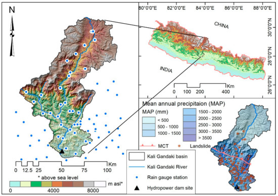
Figure 1.
Location of the Kali Gandaki (KG) River basin superimposed with a network of rain gauge stations. The shaded background is the elevation (SRTM, Shuttle Radar Topography Mission at 90 m spatial resolution). The bottom right panel shows the mean annual precipitation (MAP) for the period of 2006–2019 computed using 77 rain gauge stations distributed across the KG River basin and the reported landslides for the same period.
2. Materials and Methods
2.1. Study Area
We chose the KG River basin (area = 7560 km2) as our case study area because of a comparatively dense network of existing rain gauge stations and the availability of daily SSC and streamflow records. The sediment monitoring of the Nepalese rivers is often limited, and wherever the sediment data are available, they are typically limited to a few years. The KG River is a snow/glacier-fed river originating from the Himalayas near Tibet′s border (China) and Nepal (Figure 1). The river flows from north to south, traverses the country′s width and passes through the deepest gorge in the Himalayas and hilly regions, joins the Narayani River in southern Nepal, and enters the Terai plains of the country and finally merges with the Ganges River in India.
Figure 1 shows the study area′s location and underlain topography. The figure also depicts the spatial variation of mean annual precipitation (MAP) with topographic elevations. The river flows through sheer-sided, and deep ravine topographical settings and widens at the locations where the Himalayan range begins to close in. The KG river traverses through the world′s deepest gorge, which separates the eight thousand massifs; Dhaulagiri (on the west) and Annapurna (on the east) [27]. The upper part of the gorge is a Trans-Himalayan region characterized by high wind speed [28,29].
The physiography of the KG River basin comprises major tectonic units of the Himalayas, which include Lesser and Greater Himalayan Sequence, and Tibetan (Tethyan) Sedimentary Sequence. The main central thrust (MCT) shown in Figure 1 separates the Lesser and Greater Himalayas, and most of the landslides are located across and nearby the MCT [30]. The study area encountered several large landslides/debris flows in recent history in 1988, 1989, 1998, and 2015 triggered by Talbagar debris slide, Tatopani wedge failure, Baisari landslides, and Dhampus-Kalopani rock avalanche, respectively [31]. In addition, the blasting and excavation activities related to new road construction along the KG River basin have weakened the rock surfaces and increased the landslide and slope-failures risk [15]. The upper part of the KG basin represents the country′s driest region (with MAP less than 500 mm) due to the strong orographic barrier. The Annapurna mountain′s windward side is the wettest region of the country (Lumle with MAP greater than 5000 mm) [10]. Therefore, hydroclimatic and sedimentological variations are the results of diverse topographical and geological settings coupled with several anthropogenic causes.
2.2. Data
This study explores the changes in streamflow and sediment flux for 2006–2019. We used mean daily discharge (MDD) and daily SSC upstream of the KG hydropower project dam site, maintained by Nepal Electricity Authority (NEA). The dam construction started in 1997 and was completed in 2002. The NEA measures sediment samples and water levels daily, and flow velocity monthly (refer to Scheme A1 in the Appendix A). The NEA processes these raw data to estimate MDD and daily SSC. We computed the annual average and annual maximum MDD, and annual average and annual maximum SSC were computed from the respective time series data.
We used 24-h accumulated (daily) precipitation data of 77 rain gauge stations maintained by the Department of Hydrology and Meteorology (DHM) over the KG River basin for analysis. DHM uses a traditional US standard (8″diameter) manual rain gauges, where a local observer measures daily precipitation every day at 03 UTC (8:45 local time) [32]. We computed precipitation indices (shown in Table 1) from the daily precipitation observations. RX1day is the absolute index corresponding to the maximum 1-day precipitation, while RX3day, RX5day and RX7day are absolute indices corresponding to maximum consecutive 3-day, 5-day and 7-day precipitation of the year, respectively. R10, R20, R50, and R100 are threshold-based indices referring to the count of days in a year exceeding daily precipitation of 10, 20, 50, and 100 mm, respectively. In terms of soil erosion, an erosive event is generally defined as the rainfall event with more than 12 mm of total rainfall accumulation [33], and in the lack of sub-daily rainfall data, de Santos Loureiro and de Azevedo Coutinho [34] obtained a satisfactory relationship for estimating rainfall erosivity using the information of R10. Talchabhadel et al. [35] found that daily precipitation >10 mm could be used as a proxy for estimating soil erosion in Nepal′s hilly catchments. Therefore, the selection of R10 as a minimum threshold is a suitable basis for this study.

Table 1.
Precipitation indices used in this study.
Pokharel et al. [12] conducted a frequency analysis of daily precipitation ranging from 50 mm to 300 mm over the entire country. They showed that very heavy precipitation (>200, >250, and >300 mm/day) events increased in recent years (i.e., after 2000). Various types of flood (e.g., river floods, flash floods, and urban floods) and inundation events normally occur during RX1day, RX3day, RX5day and RX7day. The PRCPTOT is the total precipitation amount in a year. Four ratio-based indices were deduced from absolute indices (RX1day, RX3day, RX5day, and RX7day) and PRCPTOT, which provide a clear idea of fluctuations of annual precipitation total, annual extremes, and their interactions. Overall, they depict the percentage contribution of the absolute indices (RX1day, RX3day, RX5day, and RX7day) to the PRCPTOT in a particular year. We computed standard deviation (STD) and coefficient of variation (CV) for all indices across years to represent inter-annual variability. For instance, the higher values of STD and CV represent bigger inter-annual fluctuation.
We compiled the recorded landslides across the study basin from 2006 to 2019 from the database [36], which was constructed using a wide range of sources, including technical and newspaper reports. Often, it could be seen that precipitation triggered the compiled landslide events. However, the co-seismic landslide records have not been included in the catalog maintained by Pradhan et al. [36]. We computed the Normalized Difference Vegetation Index (NDVI) using Landsat images (spatial resolution 30 m and temporal resolution 16-days) in Google Earth Engine (GEE) platform. We used Thematic Mapper (Landsat 5) and Operational Land Imager (Landsat 8) sensors to compute NDVI values. NDVI informs the vegetation greenness and can be used to delineate bare land. NDVI is computed using the reflectance values corresponding to the near infrared and red bands. The annual NDVI maps were developed using the median NDVI values from images taken every 16-days of the year. Areas with NDVI values ranging from 0 to 0.15 were delineated as bare land.
2.3. Methods
Spatial distribution maps of different indices and their inter-annual variations (STD and CV) were generated by interpolating the corresponding station recordings in ArcGIS using the universal kriging method with linear drift semivariogram model. Ordinary kriging is a constant (stationary) mean in the local neighborhood of each estimation point [37] and local variance within the search region (spherical, circular, exponential, gaussian, or linear) is used for estimation. The universal kriging assumes that the unknown mean has functional dependence on the spatial location. This method splits the random function into a linear combination of deterministic functions, the smoothly varying and non-stationary trend (i.e., drift) and a random residual function [38]. Karki et al. [39] showed that both precipitation and temperature show a spatial trend structure, that is dependent on latitude, longitude, and elevation across Nepal justifying the selection of the universal kriging method.
We computed basin-averaged value using “zonal statistics” in the ArcGIS platform to assess the association of precipitation indices with streamflow and sediment yield. Correlations among selected basin-averaged precipitation indices, streamflow, and sediment runoff were computed using Pearson’s correlation coefficient. The statistical significance was checked at a 99% confidence level. Flow duration curves for both streamflow and sediment were generated by organizing all daily data of specific periods in descending order. We divided the flow duration curves into four different zones based on their probability of exceedance (PoE). The PoE informs the percentage of the time the flow is equaled or exceeded. The categories we defined are; (i) extremely high (PoE = 0–1%), (ii) high (PoE = 1–10%), (iii) average (PoE = 10–60%), and (iv) low (PoE = 60–100%).
The study period was carefully categorized into three groups: 2006–2009, 2010–2014 and 2015–2019 to represent the different phases of development activities (e.g., road construction) in the KG River basin. The first period (i.e., 2006–2009) represents the completion and opening of Kali Gandaki Road. The second and third periods are before and after the Gorkha Earthquake (25 April 2015). Though our focus in this study is not on seismic activity, we disaggregate the period because significant landslides were triggered during and after the Gorkha Earthquake.
The relationship between precipitation, SSC, and streamflow was explored for those three periods. Finally, a sediment rating curve was generated for the study area using the power-law relationship as shown in Equation (1).
where, and are variables of interest, is the law′s exponent, and is a constant. Since SSC is predicted using the information of MDD, we fitted the relation as below:
We randomly disaggregated the daily SSC and MDD data into training (70%) and testing (30%). Nash–Sutcliff efficiency (NSE), coefficient of determination (R2), and percentage bias (PBIAS) of predicted SSC were computed with respect to observed SSC for both training and testing data on daily and monthly scales.
where, and are observed and predicted SSC values, respectively. NSE is a normalized index that delivers the magnitude of residual variance with respect to observed variance [40]. NSE value ranges from −∞ to 1. NSE values equal to 1 denote a perfect estimation of the prediction. R2 informs the correlation between observed and predicted series and the range of R2 is 0 to 1. Values closer to 1 indicated a high correlation. PBIAS is the percentage difference between observed and predicted series with respect to observed data. A positive value of PBIAS represents overestimation whereas a negative value represents underestimation.
This study also explored instances that recorded higher SSC values and/or streamflow and explored if we could associate it with selected precipitation indices and other possible anthropogenic and/or natural causes. We selected 50 such instances (~top 1 percentile) based on larger SSC values and finally extracted the corresponding data of streamflow and precipitation (24 h, cumulative 3-day, 5-day and 7-day). We randomly disaggregated the selected 50 instances into training (70%) and testing (30%). This allows us to characterize the extreme SSC instances using the precipitation indices as a proxy for the KG basin.
3. Results
This section presents key results from the analysis of precipitation indices, streamflow and sediment flux data.
3.1. Spatio-Temporal Variability
We assess the spatial distribution of mean annual values of R10, R20, R50, and R100 for the period of 2006–2019 (refer to Figure 2 left panel). The upper part of the KG basin, which is located on the mountain′s leeward side, has a few rainy days and a very few heavy precipitation days.

Figure 2.
Spatial distribution of mean values of the annual count of days with daily precipitation ≥10, 20, 50, and 100 mm (denoted by R10, R20, R50, and R100, respectively in the left panel) and yearly maximum precipitation amount of 1 day, consecutive 3, 5 and 7 days (denoted by RX1day, RX3day, RX5day, and RX7day, respectively in the right panel) across the Kali Gandaki River basin. Each plot of precipitation index has two plots: one for STD (temporal standard deviation) and another for CV (temporal coefficient of variation) for 2006–2019. A description of the precipitation indices is shown in Table 1.
Based on the mean annual values, we find that there were only ~5 days of R10, ~2 days of R20, no days of R50 and R100 at the basin’s driest region. The wettest region showed ~116 days of R10, ~76 days of R20, ~33 days of R50, and ~10 days of R100. Such a diverse variation of extreme precipitation could lead to different yields of sediment runoff across the basin. For example, 10 out of 77 stations showed only 25 days in a year with daily precipitation exceeding 10 mm. In contrast, 5 out of 77 stations showed more than 100 days in a year with daily precipitation exceeding 10 mm. In terms of extremely heavy precipitation days (i.e., R100), we found that almost 60% of the stations (45 out of 77) comprise at least one day with R100. During such extreme events, a huge amount of sediment is often washed away from the basin. Along with the spatial variation, the study basin exhibits a significant inter annual variation (expressed using STD and CV in Figure 2).
We highlight instances of RX1day, RX3day, RX5day, and RX7day in Figure 2 (right panel). They represent the spatial distribution of 1-day maximum precipitation, and consecutive 3-day, 5-day and 7-day maximum precipitation. Larger surface runoff and sediment load are typically represented by this information, which we discuss in the subsequent sections. As expected, there is a significant spatial variation of these indices across the basin. The wettest region in the basin typically receives ~210 mm precipitation in a day, ~435 mm in consecutive three days, ~543 mm in consecutive five days, and ~658 mm in consecutive seven days in a year. In contrast, the driest region in the basin gets only ~38 mm for RX7day. Thus it is reasonable to expect a wide variation in the precipitation-induced sediment yield.
We show the inter-annual variation of basin-averaged precipitation, streamflow, SSC anomaly along with the bare land area anomaly of the KG basin in Figure 3a–d. Although we see a substantial inter annual variation of several precipitation indices (not shown), we highlight only a few in Figure 3. Most of the extreme precipitation indices are associated with instantaneous events. We deal with these instances in the subsequent section and focus on annual sediment yield in the current section. In general, the tendency of precipitation and streamflow is congruous with a slight fluctuation in a few years. Although the sediment transport is guided by streamflow, we find a significant discrepancy between SSC and streamflow tendencies. There is a clear positive anomaly of SSC from 2006 to 2010, which is quite different in streamflow. Multiple factors control the sediment supply and transport in the Himalayan basin; a straight-forward and simple analysis (shown in Figure 3) is insufficient. Bare land areas are prone to produce more sediment yield. We find that the trends of SSC are quite similar to the trends of bare land areas. The resulting Pearson’s correlation between the two was found to be 0.6, indicating a moderate association. Landslide is another crucial source of sediment yield. Figure 3e presents the annual count of reported landslides in the KG River basin (also refer to Figure 1). Despite a fluctuating pattern, we could detect a general increasing tendency of the occurrence of landslides. Here, we did not consider the size of landslides, and their stability after the occurrence. It is envisaged that such information in conjunction with the amount, intensity, and frequency of extreme precipitation locally affect the sediment yield. In the subsequent section, we attempt to explore other possible anthropogenic causes, such as road construction and land-use/land-cover (LULC) changes in relation to the sediment yield of the basin. Before that, we investigate the correlation of streamflow and SSC with all precipitation indices in order to quantify climatic association and causes.

Figure 3.
Anomaly plots of annual values of (a) precipitation, (b) suspended sediment concentration (SSC), (c) streamflow, and (d) bare land area (NDVI = 0 to 0.15) from 2006 to 2019. Blue color represents a positive anomaly meaning greater than the average for 2006 to 2019, whereas red color represents a negative anomaly. (e) Annual count of reported landslides during the study period (refer to Figure 1).
3.2. Correlation
Figure 4 shows a summary of the correlation among basin-averaged precipitation indices, streamflow, and sediment flux. In general, PRCPTOT shows a positive correlation with all threshold-based indices, extreme precipitation amount-based absolute indices and streamflow, but no correlation with SSC. Since ratio-based indices are computed using the PRCPTOT as a denominator, they negatively correlate with PRCPTOT. Notably, PRCPTOT demonstrates a significant correlation (at p = 0.01) with R20, R50, and RX7day, and a moderate correlation with R10, RX5day, and average MDD.

Figure 4.
Pearson′s correlation among different precipitation indices, fluvial/sediment discharge parameters (i.e., maximum and average SSC), and streamflow parameters (i.e., maximum and average MDD). Cross values represent statistically insignificant at p = 0.01. Pies and colors denote correlation values. A description of precipitation indices is shown in Table 1.
We observe maximum SSC has a significant positive correlation with RX3day only, whereas average SSC shows a statistically significant positive correlation with all ratio-based indices. In streamflow, maximum MDD has a significant correlation with extreme precipitation amounts based on absolute indices, such as RX1day, RX3day, RX5day, and RX7day. In contrast, average MDD shows less association with these absolute indices. However, we find an interesting significant association of average MDD with R20. Apart from R20, average MDD has positive correlations with R10, and R50, although it is statistically insignificant at p = 0.01.
3.3. Relationship between Streamflow, Suspended Sediment Concentration (SSC), and Precipitation
We show the flow duration curves of streamflow and SSC in Figure 5 highlighting four different PoE zones during 2006–2009, 2010–2014, and 2015–2019.
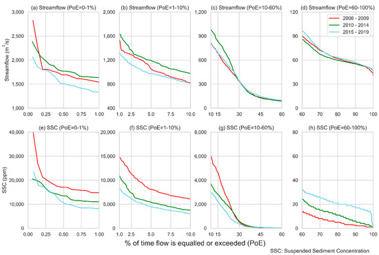
Figure 5.
Flow duration curves showing the probability of exceedance (PoE) during three periods (2006–2009 in red, 2010–2014 in green, and 2015–2019 in blue) for streamflow (upper panels (a–d)) and suspended sediment concentration (lower panels (e–h)) at Kali Gandaki hydropower reservoir site. First, second, third, and fourth columns from left represent PoE ranging 0–1 (extremely high flow), 1–10 (high flow), 10–60 (average flow), and 60–100 (low flow) respectively.
For the extremely high zone (PoE ≤ 1%) and high zone (1% > PoE ≤ 10%), sediment transport during 2006–2009 was noticeably larger compared to the other two periods. However, the streamflow did not reveal such a footprint in these zones. In other words, it highlights that the sediment transport during 2006–2009 is not only dominantly governed by hydroclimatic causes (precipitation and streamflow) but could also be due to the increased sediment yield during 2006–2009 because of different anthropogenic activities. Despite the Gorkha earthquake, we could not find signatures of an increased SSC during 2015–2019. We highlight some of the major anthropogenic activities in the following section. The noticeably larger value of SSC in 2006–2009 continues up to PoE ≅20%. Extreme precipitation, instantaneous streamflow and instantaneous SSC are spatially as well as temporally local. The extreme instances are unique and have unusual characteristics with significant uncertainties. Apart from these extreme instances, the SSC showed a congruous trend of streamflow, in general. Thus the average sediment transport or annual/seasonal sediment yield could be predicted as a function of streamflow. We could see that both the streamflow and SSC are slightly larger during 2010–2014 than in 2015–2019.
In Figure 6, we show the daily variation of SSC, streamflow and precipitation for August 2009, which includes the day with the highest recorded daily SSC during the study period. A 3-day lag of precipitation to the peak of streamflow and SSC could be seen. The figure also highlights that the basin-averaged precipitation is about one-fourth to one-fifth of the maximum daily precipitation recorded by any study basin station. In general, the alteration of streamflow is guided by the variation of basin-averaged precipitation. However, the fluctuation of SSC sometimes shows a slightly different trend. This may be attributed to significant variation of precipitation across the study basin.
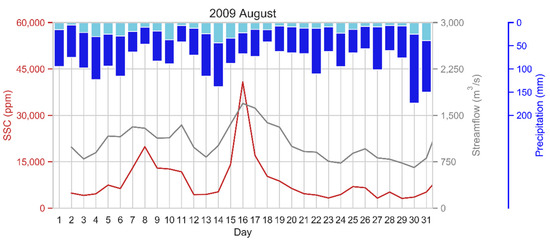
Figure 6.
Daily variation of suspended sediment concentration (SSC), streamflow, and precipitation for August 2009. The highest recorded SSC during the entire study period was 40,801 ppm. Sky blue color represents basin averaged daily precipitation of the study area. In contrast, the dark blue color represents the maximum value of daily precipitation recorded by any precipitation station located inside the study basin. In general, basin-averaged daily precipitation is about 20–25% of the study basin’s maximum daily precipitation. We analyzed other instances too, but did not show them here for brevity.
Though spatially averaged, we investigate the association of different selected indices with the top 1 percentile SSC (extreme) instances. The randomly disaggregated training and testing data revealed that the average basin precipitation (1-day, consecutive 3-day, 5-day, and 7-day) has a wide variation for extreme instances (refer to Figure 7). Thus, it is not always straightforward that the heavy precipitation will result in larger sediment and/or streamflow and vice-versa. Generally, the KG River basin showed that for these top 1 percentile SSC instances, the consecutive 5-day basin-averaged precipitation is about 85–90 mm and the consecutive 7-day basin-averaged precipitation is about 110–120 mm. Table A1 in the Appendix A provides the details of these indices during training and testing for the top 1 percentile SSC instances. The table shows that the basin-averaged 24 h precipitation of about 25 mm resulted in the top 1 percentile SSC instances. In other words, assuming that the maximum daily rainfall at the wettest station across the study basin is four to five times basin-averaged precipitation, such instances could be generated if daily precipitation is greater than 100–25 mm.
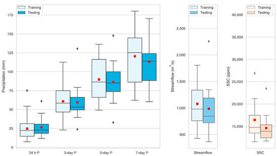
Figure 7.
Boxplots showing the variation of basin averaged precipitation (1-day, 3-day cumulative, 5-day cumulative, and 7-day cumulative), suspended sediment concentration (SSC), and streamflow of top 50 larger daily SSC values for the period from 2006 to 2019. The red square indicates the average value and the boxplot shows quantiles (Q1 and Q3), median (Q2) and range of variation. The data were randomly sliced into calibration (70%) and validation (30%).
3.4. Prediction of Sediment Yield
We discussed earlier that the quantitative prediction of SSC is challenging. However, the average SSC and seasonal/annual sediment yield could be predicted by carefully evaluating the relationship between streamflow and SSC. Using the scatter plots of precipitation, streamflow, and SSC, we found that the SSC had a close association with the streamflow. The power-law relationship held a better agreement (refer to Figure A1 for SSC-streamflow plot). If our interest is to predict for a specific period, then these relations should be updated for different periods. For instance, Figure A1 shows that a slightly different relationship might be needed for 2006–2009.
In this study, we develop a predictive relationship that can estimate the sediment budget to evaluate the seasonal/annual sediment yield across the study basin or fill the SSC data gaps (if any). In addition, under changing climate such a simple relation could estimate likely future sediment yield. The developed model based on the power-law relationship is shown in Table 2.
Table 2.
Suspended sediment concentration (SSC) prediction using power-law relationship in Kali Gandaki (KG) River at KG hydropower project dam site and the performance metrics on a daily scale.
The coefficient of determination (R2) for daily data was found to be 0.42 for both training and testing data. Percentage bias (PBIAS) was about −20%, meaning the predictions underestimated the observations by 20%. The Nash-Sutcliffe Efficiency (NSE) based on daily data was found to be 0.35. On a monthly scale, R2 was found to be 0.71 and NSE was found to be 0.63. The comparison plot between observed and predicted daily SSC data is shown in Figure A2 in the Appendix A. We deem the values of performance metrics acceptable for the prediction of sediment yield [41].
3.5. Sediment Yield and Its Relationship with Anthropogenic Activities and Natural Hazards
Generally, road construction in mountain regions involves a major cut of hills and a partial filling. We find from the earth-work data of eight sample hill roads (refer to Table A2 in Appendix A) inside the KG River basin. Only 15% to 30% of soil cutting was used to fill, and the surplus is washed away and transported towards the KG River during heavy precipitation. It was found that about 3000 m3 of surplus sediment is deposited nearby construction sites on every unit km of road construction. The KG corridor was opened in 2008 [42] and is currently upgraded to a two-way tarred road as a part of the KG Road Corridor [43]. The KG Road Corridor connects China and India.
A sample of the spatial distribution of NDVI for the year 2010 is shown in Figure A3 (Appendix A). The figure also shows a visual comparison between the bare land predicted using NDVI and LULC classification developed by the ICIMOD. The model works reasonably well in representing the bare land areas. However, some agricultural lands are delineated in the range of NDVI values from 0 to 0.15. Depending on the cultivated crops and times of the year, agricultural land has different greenness values. Changes in vegetation and deforestation due to LULC changes or road construction are captured by a decrease in NDVI values. However, note that the resolution of NDVI information is limited to 30 m. We find the inter-annual variation of bare land areas (i.e., areas with NDVI = 0 to 0.15) clearly showed larger values from 2006 to 2011. The trend of increased SSC parallels the increase in bare land areas.
Furthermore, a single instance of a massive landslide in the early morning of 24 May 2015, buried a village of 25 houses (fortunately no human casualties). The landslide was a dry type landslide and was weakened by 25 April 2015, main-shock and subsequent aftershocks [44]. The massive landslide, ~50 km upstream of the KG Hydropower project, completely blocked the river forming an artificial earth dam [18]. The artificial lake extended approximately 1–3 km upstream of the temporary dam and water started overflowing only after 16 hrs. After the landslide, water kept a steady flow without causing major damage or casualties downstream. This example illustrates that even a single disastrous incident could bring a considerable amount of sediment.
4. Discussion
The spatio-temporal variation of seasonal and extreme precipitation is significant in the KG basin. Sound understanding of the variability of these precipitation indices is crucial for managing downstream river reach. Dahal and Hasegawa [45] reported that the risk of landslides on Himalaya mountain slopes is high when the daily precipitation exceeds 144 mm. Most of the analyzed stations showed that the threshold was reached multiple times, which shows the possibility of the occurrence of rainfall-induced landslides in the study basin. In some years, at a few stations, we also found that the maximum 7-day consecutive precipitation exceeded 1000 mm. These instances could be responsible for a larger sediment transport locally for a specific time, as discussed by Upadhayay et al. [46] potentially explaining the larger uncertainty at the upper tail (see Figure A2). However, since we do not have sediment monitoring stations other than at the basin′s outlet, the source′s spatial variability and transport of sediments are difficult to explore. If there were multiple hydrometric stations, the hydrodynamic routing of flow and sediment could inform a travel time of water and sediment from several sources during normal and extreme cases.
Annual precipitation showed a positive correlation with threshold-based indices (R10, R20, R50, and R100), absolute indices (RX1day, RX3day, RX5day, and RX7day), and streamflow but did not show correlation with SSC. The anomaly and correlation plots highlight that the SSC is challenging to predict using only the annual precipitation. However, the average SSC showed a clear correlation with streamflow and ratio-based precipitation indices. Since there is a strong dependence of sediment concentration primarily on streamflow, we established a relationship between SSC and MDD on a daily scale. Since sediment transport measurements are labor-intensive and expensive in terms of both cost and time [47], sediment yield is typically predicted using different physically-based, empirical or statistical models [18,48,49]. The developed power-law relationship demonstrated a much better estimation (R2 > 0.7) for monthly SSC and a fair estimation (R2 ~ 0.4) for daily SSC. Bajracharya et al. [50] reported that precipitation and streamflow are expected to increase due to climate change in the KG River basin. Therefore, a study on sediment transport under changing climate would be interesting for prospective researchers.
Higher SSC values are not captured by modeling alone [51]. Examination at extreme sediment transport instances and correlation plots reveals that the peak SSC events moderately correlated with consecutive 3-day precipitation. Most of those extreme instances occurred with over 60 mm basin-averaged consecutive 3-day precipitation. In general, the maximum precipitation is about four to five times of basin-averaged precipitation. Therefore, consecutive 3-day precipitation of about 250–300 mm at any stations could be an alarming scenario for higher SSC at the basin′s outlet.
There could be localized extreme sediment production and/or extreme precipitation, which control the sediment transport. More than 50% of total annual soil erosion occurred in just one or two major extreme precipitation events [52] in Nepal′s mountainous basins. The changes in NDVI inform vegetation changes, road construction, and other anthropogenic activities. Since bare land areas are more susceptible to producing higher sediment yield, we emphasized annual changes in bare land areas of the KG River basin. In general, the years with larger areas of bare land showed higher sediment yield.
Analysis of physical mechanisms for the increment of bare land areas in some years was not done. However, we found that the increase of bare lands was concomitant with increased road construction around these years. The reported landslides do not have information on the sizes of landslides, and the accuracy of their spatial location is not precise enough. Therefore, we did not carry out their spatial analysis. In the future, we plan to map all landslides (both seismic and non-seismic) with their sizes, enlist all constructed roads and their earthworks, and associate them with different precipitation indices.
It is clear from the analysis that the sediment transport is predominantly guided by streamflow and precipitation. Nevertheless, the SSC prediction at the upper tail is challenging in Himalayan basins. The extreme sediment transport events are likely driven by both extreme precipitation and detrimental anthropogenic activities. Therefore, we feel an urgency in sediment source management on mountain slopes of the Nepal Himalaya to control the extreme SSC events.
5. Conclusions
Streamflow and sediment yield alterations reflect several drivers′ integrated response, including hydrometeorological, geomorphological, and other natural and anthropogenic factors such as LULC, landslides, and road constructions. Streamflow is comparatively easy to predict with the information on catchment characteristics and precipitation. However, sediment yield is challenging to predict in Himalayan river basins because sediment transport is dependent on multiple factors and understanding the physical mechanisms and interrelation with other drivers is challenging. The average sediment budget could be predicted to some extent, as we illustrate in this study. Here we attempted to explain SSC variation with hydroclimatic (such as precipitation) and anthropogenic activities (such as road construction).
The spatial variation of precipitation (both annual and extreme) is significant across the KG River basin. Streamflow showed a good correlation with different precipitation indices. However, SSC demonstrated a weak correlation with these indices. Interestingly, we found that the extreme SSC had a positive correlation with RX3day and the average SSC had a positive correlation with the ratio-based precipitation indices (such as RX1day/PRCPTOT, RX3day/PRCPTOT).
Basin averaged precipitation was only one-fourth to one-fifth of maximum precipitation in the wettest region. While analyzing the top 1 percentiles (~50 instances) of SSC, our study found that the basin-averaged consecutive 1-day, 3-day, 5-day and 7-day precipitation were 25 mm, 60 mm, 90 mm, and 120 mm, respectively during those instances. If we consider the spatial variability of precipitation across the study basin, 1-day precipitation of > 100 mm, 3-day precipitation of > 250 mm, 5-day precipitation of > 350 mm, and 7-day precipitation of > 500 mm could produce an alarming scenario of larger SSC in smaller sections of the river.
In the KG River basin, we proposed a power-law relationship between the SSC and daily stream flow and found R2 of 0.4 on a daily scale and 0.7 on a monthly scale and NSE of 0.35 on a daily scale, and 0.63 on a monthly scale. The overall prediction was found to be underestimated by 20% to observed SSC. The extreme SSC could not be predicted as well with this relationship for several reasons we discussed above. The tendency of inter annual variation of SSC was supported by the tendency of inter annual variation of bare land areas (at a moderate correlation with R = 0.6) that were computed using NDVI from Landsat observations. The results demonstrate that the NDVI could be used as a good overall proxy to connect several anthropogenic activities.
We noticed that even a single instance could bring large sediment loads either from soil erosion or landslides or washed earthworks or combinations thereof. Several development activities are underway in the Himalaya basins, particularly the construction of non-engineered roads. Under a changing climate, the severity and frequency of extreme precipitation are expected to increase, which could potentially wash away and produce more sediment flux in the future. Therefore, watershed management at mountain slopes is necessary along with river channel improvement and sediment management in the mountainous river basins. We recommend and integrated planning of sediment management, considering extreme hydroclimatic instances and anthropogenic disturbances. In this quest, both point and areal sources of sediment require careful analysis.
Author Contributions
Conceptualization, R.T.; methodology, R.T., J.P., S.S., and G.R.G.; software, R.T.; formal analysis, R.T.; investigation, R.T., R.B., J.P., S.S., G.R.G., P.D., K.D., K.R.G., and B.P.; resources, R.T., R.B., M.B.B., S.K.C., B.J., S.K. (Surendra Kaini), and B.P.; data curation, R.T. and R.B.; writing—original draft preparation, R.T.; writing—review and editing, R.T., R.B., J.P., S.S., G.R.G., P.D., M.B.B., K.D., K.R.G., B.P., and S.K. (Saurav Kumar). All authors have read and agreed to the published version of the manuscript.
Funding
This research received no external funding.
Data Availability Statement
The data used in this study will be provided on request.
Acknowledgments
The authors greatly acknowledge the Department of Hydrology and Meteorology (DHM), Nepal and the Nepal Electricity Authority (NEA), Nepal for providing the hydrometeorological and sediment data used for the study. The authors are grateful to the anonymous reviewers for their reviews and constructive comments.
Conflicts of Interest
The authors declare no conflict of interest.
Appendix A

Scheme A1.
(a) Kali Gandaki river upstream of hydropower dam (b) sedimentation downstream of weir, (c) a staff of Kali Gandaki Hydropower project sampling water for sediments, and (d) measuring weight of dry sediment to compute suspended sediment concentration.

Figure A1.
Sediment rating curve generated using daily streamflow and suspended sediment concentration (SSC) for three periods.

Figure A2.
Comparison plot of observed and predicted daily suspended sediment concentration (SSC) from 2006 to 2019 for Kali Gandaki (KG) River at KG hydropower dam site.

Figure A3.
Spatial distribution of Normalized Difference Vegetation Index (NDVI), bare land predicted using NDVI values, and land use/land cover for the year 2010. The LULC map for the year 2010 was produced by the International Centre for Integrated Mountain Development [53] at a spatial resolution of 30 m, and details are available in Uddin et al. [54]. NDVI was computed as (NIR − Red)/(NIR + Red) where NIR = near infrared band reflectance and Red = red band reflectance from Landsat observations.
Table A1.
Average values of precipitation (24 h, 3-day cumulative, 5-day cumulative, and 7-day cumulative), suspended sediment concentration (SSC), and streamflow of top 50 larger daily SSC values for the period from 2006 to 2019.
Table A1.
Average values of precipitation (24 h, 3-day cumulative, 5-day cumulative, and 7-day cumulative), suspended sediment concentration (SSC), and streamflow of top 50 larger daily SSC values for the period from 2006 to 2019.
| Training (70%) | Testing (30%) | |
|---|---|---|
| 24 h precipitation (mm) | 24.7 | 26.4 |
| 3-day precipitation (mm) | 60.9 | 59.4 |
| 5-day precipitation (mm) | 89.8 | 86.2 |
| 7-day precipitation (mm) | 120.5 | 113.3 |
| SSC (ppm) | 16,474.3 | 14,630.6 |
| Streamflow (m3/s) | 1078.1 | 984.8 |
Table A2.
Summary of earthworks of constructed/upgraded road in Kali Gandaki basin.
Table A2.
Summary of earthworks of constructed/upgraded road in Kali Gandaki basin.
| SN | Name of Road | Length (Km) | Cutting (m3) | Filling (m3) | Surplus (m3) |
|---|---|---|---|---|---|
| 1 | Mudikuwa-Jhaklak-Kurgha-Lunkhu | 6.7 | 81,637 | 12,236 | 69,401 |
| 2 | Waling-Huwas | 7.5 | 17,974 | 2503 | 15,471 |
| 3 | Rangkhola-Biruwa | 10 | 14,618 | 2839 | 11,779 |
| 4 | Badhkhola-Taksar-Dulegauda | 10 | 11,526 | 1399 | 10,127 |
| 5 | Putalikhet-Aruchaur | 6.6 | 12,319 | 2467 | 9852 |
| 6 | Naudanda-Karkineta | 10 | 15,003 | 3014 | 11,989 |
| 7 | Gumti-Chisapaani | 6.18 | 53,535 | 15,297 | 38,238 |
| 8 | Helu-Arjunchaupari | 8.2 | 23,505 | 729 | 22,776 |
References
- Walling, D. The changing sediment loads of the world’s rivers. Ann. Wars. Univ. Life Sci.-SGGW Land Reclam. 2008, 39, 3–20. [Google Scholar] [CrossRef]
- Zhao, G.; Mu, X.; Strehmel, A.; Tian, P. Temporal variation of streamflow, sediment load and their relationship in the Yellow River basin, China. PLoS ONE 2014, 9, e91048. [Google Scholar] [CrossRef]
- Chang, Q.; Zhang, C.; Zhang, S.; Li, B. Streamflow and sediment declines in a loess hill and gully landform basin due to climate variability and anthropogenic activities. Water 2019, 11, 2352. [Google Scholar] [CrossRef]
- Gautam, M.R.; Acharya, K. Streamflow trends in Nepal. Hydrol. Sci. J. 2012, 57, 344–357. [Google Scholar] [CrossRef]
- Wang, S.; Zhang, Z.R.; McVicar, T.; Guo, J.; Tang, Y.; Yao, A. Isolating the impacts of climate change and land use change on decadal streamflow variation: Assessing three complementary approaches. J. Hydrol. 2013, 507, 63–74. [Google Scholar] [CrossRef]
- Ye, X.; Zhang, Q.; Liu, J.; Li, X.; Xu, C. Distinguishing the relative impacts of climate change and human activities on variation of streamflow in the Poyang Lake catchment, China. J. Hydrol. 2013, 494, 83–95. [Google Scholar] [CrossRef]
- Wulf, H.; Bookhagen, B.; Scherler, D. Climatic and geologic controls on suspended sediment flux in the Sutlej River Valley, western Himalaya. Hydrol. Earth Syst. Sci. 2012, 16, 2193–2217. [Google Scholar] [CrossRef]
- Wang, S.; Fu, B.; Piao, S.; Lü, Y.; Ciais, P.; Feng, X.; Wang, Y. Reduced sediment transport in the Yellow River due to anthropogenic changes. Nat. Geosci. 2016, 9, 38–41. [Google Scholar] [CrossRef]
- Wang, G.; Zhang, J.; Li, X.; Bao, Z.; Liu, Y.; Liu, C.; He, R.; Luo, J. Investigating causes of changes in runoff using hydrological simulation approach. Appl. Water Sci. 2017, 7, 2245–2253. [Google Scholar] [CrossRef]
- Talchabhadel, R.; Karki, R.; Thapa, B.R.; Maharjan, M.; Parajuli, B. Spatio-temporal variability of extreme precipitation in Nepal. Int. J. Climatol. 2018, 38, 4296–4313. [Google Scholar] [CrossRef]
- Shrestha, D.; Singh, P.; Nakamura, K. Spatiotemporal variation of rainfall over the central Himalayan region revealed by TRMM precipitation radar. J. Geophys. Res. Atmos. 2012, 117. [Google Scholar] [CrossRef]
- Pokharel, B.; Wang, S.-Y.S.; Meyer, J.; Marahatta, S.; Nepal, B.; Chikamoto, Y.; Gillies, R. The east–west division of changing precipitation in Nepal. Int. J. Climatol. 2020, 40, 3348–3359. [Google Scholar] [CrossRef]
- Wang, S.W.; Gebru, B.M.; Lamchin, M.; Kayastha, R.B.; Lee, W.-K. Land use and land cover change detection and prediction in the Kathmandu district of Nepal using remote sensing and GIS. Sustainability 2020, 12, 3925. [Google Scholar] [CrossRef]
- Bhandari, S.B.; Shahi, P.B.; Shrestha, R.N. Overview of rural transportation infrastructures in Nepal. Eurasia J. Earth Sci. Civ. Eng. 2012, 1, 1–14. [Google Scholar]
- McAdoo, B.G.; Quak, M.; Gnyawali, K.R.; Adhikari, B.R.; Devkota, S.; Rajbhandari, P.L.; Sudmeier-Rieux, K. Roads and landslides in Nepal: How development affects environmental risk. Nat. Hazards Earth Syst. Sci. 2018, 18, 3203–3210. [Google Scholar] [CrossRef]
- Merz, J.; Dangol, P.M.; Dhakal, M.P.; Dongol, B.S.; Nakarmi, G.; Weingartner, R. Road construction impacts on stream suspended sediment loads in a nested catchment system in Nepal. Land Degrad. Dev. 2006, 17, 343–351. [Google Scholar] [CrossRef]
- Hasnain, S.I. Factors controlling suspended sediment transport in Himalayan glacier meltwaters. J. Hydrol. 1996, 181, 49–62. [Google Scholar] [CrossRef]
- Baniya, M.B.; Asaeda, T.; Shivaram, K.C.; Jayashanka, S.M.D.H. Hydraulic parameters for sediment transport and prediction of suspended sediment for Kali Gandaki river basin, Himalaya, Nepal. Water 2019, 11, 1229. [Google Scholar] [CrossRef]
- Finlayson, D.P.; Montgomery, D.R.; Hallet, B. Spatial coincidence of rapid inferred erosion with young metamorphic massifs in the Himalayas. Geology 2002, 30, 219. [Google Scholar] [CrossRef]
- Andermann, C.; Crave, A.; Gloaguen, R.; Davy, P.; Bonnet, S. Connecting source and transport: Suspended sediments in the Nepal Himalayas. Earth Planet. Sci. Lett. 2012, 351–352, 158–170. [Google Scholar] [CrossRef]
- Sohoulande Djebou, D.C. Integrated approach to assessing streamflow and precipitation alterations under environmental change: Application in the Niger River basin. J. Hydrol. Reg. Stud. 2015, 4, 571–582. [Google Scholar] [CrossRef]
- Manandhar, S.; Pandey, V.P.; Kazama, F. Hydro-climatic trends and people’s perceptions. Clim. Res. 2012, 54, 167–179. [Google Scholar] [CrossRef]
- Karki, R.; Ul Hasson, S.; Schickhoff, U.; Scholten, T.; Böhner, J. Rising precipitation extremes across Nepal. Climate 2017, 5, 4. [Google Scholar] [CrossRef]
- Karki, R.; Ul Hasson, S.; Gerlitz, L.; Talchabhadel, R.; Schickhoff, U.; Scholten, T.; Böhner, J. Rising mean and extreme near-surface air temperature across Nepal. Int. J. Climatol. 2020, 40, 2445–2463. [Google Scholar] [CrossRef]
- Suwal, N.; Kuriqi, A.; Huang, X.; Delgado, J.; Młyński, D.; Walega, A. Environmental flows assessment in Nepal: The case of Kali Gandaki river. Sustainability 2020, 12, 8766. [Google Scholar] [CrossRef]
- Uddin, K.; Abdul Matin, M.; Maharjan, S. Assessment of land cover change and its impact on changes in soil erosion risk in Nepal. Sustainability 2018, 10, 4715. [Google Scholar] [CrossRef]
- Carosi, R.; Gemignanni, L.; Godin, L.; Iaccarino, S.; Larson, K.P.; Montomoli, C.; Rai, S.M. A geological journey through the deepest gorge on Earth: The Kali Gandaki valley section, central Nepal. J. Virtual Explor. 2014, 47, 7. [Google Scholar]
- Zängl, G.; Egger, J.; Wirth, V. Diurnal winds in the Himalayan Kali Gandaki Valley. Part II: Modeling. Mon. Weather Rev. 2001, 129, 1062–1080. [Google Scholar] [CrossRef]
- Upreti, B.N.; Shakya, A. Wind energy potential assessment in Nepal. Wind Energy Potential Assess. Nepal 2016, 1, 1–4. [Google Scholar]
- Timilsina, M.; Bhandary, N.P.; Dahal, R.K.; Yatabe, R. Large-scale landslide inventory mapping in lesser Himalaya of Nepal using geographic information system. In GIS Landslide; Springer: Japan, Tokyo, 2017; pp. 97–112. [Google Scholar]
- Adhikari, B.R.; Tian, B.; Chapagain, S.; Acharya, A.; Chen, F.; Gautam, S.; Gou, X. Landslide susceptibility mapping along the Sino-Nepal road corridors: A case study of Pokhara-Korala road corridor, Nepal. Geophys. Res. Abstr. EGU 2019, 21, 1. Available online: https://meetingorganizer.copernicus.org/EGU2019/EGU2019-3220.pdf (accessed on 15 Decemeber 2020).
- Talchabhadel, R.; Karki, R.; Parajuli, B. Intercomparison of precipitation measured between automatic and manual precipitation gauge in Nepal. Measurement 2017, 106, 264–273. [Google Scholar] [CrossRef]
- Renard, K.G.; Foster, G.R.; Weesies, G.A.; McCool, D.K.; Yoder, D.C. Predicting Soil Erosion by Water: A Guide to Conservation Planning with the Revised Universal Soil Loss Equation (RUSLE); USDA ARS: Washington, WA, USA, 1997; pp. 1–384. Available online: https://www.ars.usda.gov/ARSUserFiles/64080530/RUSLE/AH_703.pdf (accessed on 15 March 2019).
- De Santos Loureiro, N.; De Azevedo Coutinho, M. A new procedure to estimate the RUSLE EI30 index, based on monthly rainfall data and applied to the Algarve region, Portugal. J. Hydrol. 2001, 250, 12–18. [Google Scholar] [CrossRef]
- Talchabhadel, R.; Nakagawa, H.; Kawaike, K.; Prajapati, R. Evaluating the rainfall erosivity (R-factor) from daily rainfall data: An application for assessing climate change impact on soil loss in Westrapti River basin, Nepal. Model. Earth Syst. Environ. 2020. [Google Scholar] [CrossRef]
- Pradhan, A.M.S.; Maharjan, B.; Silwal, S.; Sthapit, S. Preparation of Landslide Catalogue (1970–2019) of Nepal; Water Resources Research and Development Centre: Lalitpur, Nepal, 2020; pp. 1–2. Available online: http://wrrdc.gov.np/images/category/WRRDC-Research_Letter_Issue_2_November.pdf (accessed on 15 Decemeber 2020).
- Cressie, N. The origins of kriging. Math. Geol. 1990, 22, 239–252. [Google Scholar] [CrossRef]
- Wu, C.-Y.; Mossa, J.; Mao, L.; Almulla, M. Comparison of different spatial interpolation methods for historical hydrographic data of the lowermost Mississippi river. Ann. GIS 2019, 25, 133–151. [Google Scholar] [CrossRef]
- Karki, R.; Talchabhadel, R.; Aalto, J.; Baidya, S.K. New climatic classification of Nepal. Theor. Appl. Climatol. 2016, 125, 799–808. [Google Scholar] [CrossRef]
- Nash, J.E.; Sutcliffe, J.V. River flow forecasting through conceptual models part I—A discussion of principles. J. Hydrol. 1970, 10, 282–290. [Google Scholar] [CrossRef]
- Moriasi, D.N.; Arnold, J.G.; Van Liew, M.W.; Bingner, R.L.; Harmel, R.D.; Veith, T.L. Model evaluation guidelines for systematic quantification of accuracy in watershed simulations. Trans. ASABE 2007, 50, 885–900. [Google Scholar] [CrossRef]
- Beazley, R.E.; Lassoie, J.P. A Global Review of Road Development. In Himalayan Mobilities; Springer: Berlin/Heidelberg, Germany, 2017; pp. 3–28. [Google Scholar] [CrossRef]
- Bell, R.; Fort, M.; Götz, J.; Bernsteiner, H.; Andermann, C.; Etzlstorfer, J.; Posch, E.; Gurung, N.; Gurung, S. Major geomorphic events and natural hazards during monsoonal precipitation 2018 in the Kali Gandaki Valley, Nepal Himalaya. Geomorphology 2021, 372, 107451. [Google Scholar] [CrossRef]
- Hashash, Y.M.A.; Tiwari, B.; Moss, R.E.S.; Asimaki, D.; Clahan, K.B.; Kieffer, D.S.; Dreger, D.S.; Macdonald, A.; Madugo, C.M.; Mason, H.B.; et al. Geotechnical Field Reconnaissance: Gorkha (Nepal) Earthquake of April 25 2015 and Related Shaking Sequence. Report No. GEER-040. Geotechnical Extreme Event Reconnaissance Association. 2015. Available online: https://digitalcommons.calpoly.edu/cenv_fac/311/ (accessed on 28 November 2020).
- Dahal, R.K.; Hasegawa, S. Representative rainfall thresholds for landslides in the Nepal Himalaya. Geomorphology 2008, 100, 429–443. [Google Scholar] [CrossRef]
- Upadhayay, H.R.; Smith, H.G.; Griepentrog, M.; Bodé, S.; Bajracharya, R.M.; Blake, W.; Cornelis, W.; Boeckx, P. Community managed forests dominate the catchment sediment cascade in the mid-hills of Nepal: A compound-specific stable isotope analysis. Sci. Total Environ. 2018, 637–638, 306–317. [Google Scholar] [CrossRef]
- Hajigholizadeh, M.; Melesse, A.; Fuentes, H. Erosion and sediment transport modelling in shallow waters: A review on approaches, models and applications. Int. J. Environ. Res. Public Health 2018, 15, 518. [Google Scholar] [CrossRef]
- Haritashya, U.K.; Singh, P.; Kumar, N.; Gupta, R.P. Suspended sediment from the Gangotri Glacier: Quantification, variability and associations with discharge and air temperature. J. Hydrol. 2006, 321, 116–130. [Google Scholar] [CrossRef]
- Kumar, R.; Kumar, R.; Singh, S.; Singh, A.; Bhardwaj, A.; Kumari, A.; Randhawa, S.S.; Saha, A. Dynamics of suspended sediment load with respect to summer discharge and temperatures in Shaune Garang glacierized catchment, Western Himalaya. Acta Geophys. 2018, 66, 1109–1120. [Google Scholar] [CrossRef]
- Bajracharya, A.R.; Bajracharya, S.R.; Shrestha, A.B.; Maharjan, S.B. Climate change impact assessment on the hydrological regime of the Kaligandaki Basin, Nepal. Sci. Total Environ. 2018, 625, 837–848. [Google Scholar] [CrossRef] [PubMed]
- Ghorbani, M.A.; Khatibi, R.; Singh, V.P.; Kahya, E.; Ruskeepää, H.; Saggi, M.K.; Sivakumar, B.; Kim, S.; Salmasi, F.; Hasanpour Kashani, M.; et al. Continuous monitoring of suspended sediment concentrations using image analytics and deriving inherent correlations by machine learning. Sci. Rep. 2020, 10, 8589. [Google Scholar] [CrossRef] [PubMed]
- Tiwari, K.R.; Sitaula, B.K.; Bajracharya, R.M.; Børresen, T. Runoff and soil loss responses to rainfall, land use, terracing and management practices in the Middle Mountains of Nepal. Acta Agric. Scand. Sect. B Plant Soil Sci. 2009, 59, 197–207. [Google Scholar] [CrossRef]
- ICIMOD. Land Cover of Nepal 2010; ICIMOD: Kathmandu, Nepal, 2013. [Google Scholar]
- Uddin, K.; Shrestha, H.L.; Murthy, M.S.R.; Bajracharya, B.; Shrestha, B.; Gilani, H.; Pradhan, S.; Dangol, B. Development of 2010 national land cover database for the Nepal. J. Environ. Manag. 2015, 148, 82–90. [Google Scholar] [CrossRef]
Publisher’s Note: MDPI stays neutral with regard to jurisdictional claims in published maps and institutional affiliations. |
© 2021 by the authors. Licensee MDPI, Basel, Switzerland. This article is an open access article distributed under the terms and conditions of the Creative Commons Attribution (CC BY) license (http://creativecommons.org/licenses/by/4.0/).