Topology-Robust Power System Stability Prediction with a Supervised Contrastive Spatiotemporal Graph Convolutional Network

Abstract

Modern power systems face growing challenges in stability assessment due to large-scale renewable energy integration and rapidly changing operating conditions. Data-driven approaches have emerged as promising solutions for real-time stability assessment, yet their performance often degrades under network topology reconfigurations. To address this limitation, the Spatiotemporal Contrastive Graph Convolutional Network (STCGCN) is proposed for the joint task prediction of voltage and transient stability across known and unknown topologies. The framework integrates a graph convolutional network (GCN) encoder to capture spatial dependencies and a temporal convolutional network to model electromechanical dynamics. It also employs supervised contrastive learning to extract discriminative features due to the grid topology variation, enhance stability class separability, and mitigate class imbalance under varying operating conditions, such as fluctuating loads and renewable integration. Case studies on the IEEE 39-bus system demonstrate that STCGCN achieves 89.66% accuracy on in-sample datasets from known topologies and 87.73% on out-of-sample datasets from unknown topologies, outperforming single-task learning approaches. These results highlight the method’s robustness to topology variations and its strong generalization across configurations, providing a topology-aware and resilient solution for real-time joint voltage and transient stability assessment in power systems.

1. Introduction

Modern power grids are undergoing a profound transformation driven by large-scale renewable energy integration and ambitious decarbonization targets [1]. Unlike conventional systems reliant on synchronous generators, renewable-rich grids depend on inverter-based resources, such as wind and photovoltaic generation, which introduce variability, forecast uncertainty, and reduced physical inertia. These characteristics, combined with evolving demand patterns, market-driven operations, and frequent topology changes due to switching, outages, or reconfigurations, intensify nonlinear interactions and shrink stability margins [2]. Real-time stability assessment is thus essential for secure operation. Two critical aspects of system security are voltage stability, which ensures acceptable bus voltages after disturbances, and transient stability, which maintains rotor-angle synchronism following large disturbances like faults or line trips [3]. Voltage stability is increasingly challenged by limited reactive power support and weak grid conditions under high renewable penetration. Similarly, transient stability is compromised by reduced system inertia and damping due to the displacement of synchronous generators. In renewable-rich grids, these stability phenomena are tightly coupled across space and time, as active and reactive power dynamics interact through converter controls and low-inertia networks. Topology changes further complicate this coupling by altering power flows and stability boundaries. Analyzing voltage and transient stability separately overlooks these interdependencies, necessitating integrated, efficient, and adaptive assessment methods for renewable-rich, topology-varying systems.

Transient stability refers to a power system’s ability to maintain generator synchronism after major disturbances, such as short circuits, line outages, or sudden loss of generation or load [4]. It depends on the balance between mechanical input power ($P_m$) and electromagnetic output power ($P_e$), where a sustained mismatch causes rotor acceleration or deceleration, risking loss of synchronism and potentially triggering cascading failures or blackouts [5]. Voltage stability, conversely, is the ability to maintain bus voltages within acceptable limits during normal operation and after disturbances [6]. It hinges on the balance of reactive power supply and demand, influenced by load behavior, network configuration, and transmission losses. Without sufficient reactive support, heavy loading can lead to progressive voltage declines and ultimately result in collapse. In renewable-rich grids, these stability types are interconnected, as reduced voltages weaken angular stability, and rotor oscillations impact voltage recovery. These interactions, shaped by induction motor dynamics, excitation systems, network strength, and reactive power compensation, require high-fidelity modeling, typically through time-domain simulation of differential-algebraic equations (DAEs) for generators, excitation systems, loads, and compensation [7]. However, traditional computational methods face significant challenges. Conventional contingency screening solves large-scale DAEs for each scenario, often taking 5–30 min for realistic systems, which is too slow for real-time or wide-area assessment [7]. Furthermore, decoupled analysis, which evaluates voltage and transient stability separately, neglects their dynamic coupling. This is especially problematic in weak grids with high renewable penetration, reduced inertia, and variable reactive support, underscoring the need for integrated approaches to ensure accurate and timely stability assessment.

Classical control-theoretic methods have long underpinned power-system stabilization, with robust designs based on Linear Parameter-Varying (LPV) models and mixed $H_2/H_{\infty }$ synthesis offering performance guarantees under bounded uncertainties and disturbances. For example, Dehghani et al. [8] proposed a robust model predictive control (RMPC) scheme for AC microgrids that achieves effective voltage and frequency regulation via gain-scheduled state feedback. While such approaches are resilient to model uncertainty and exogenous perturbations, they typically rely on accurate plant parameters and can become computationally intractable at scale. Related advances include decentralized robust excitation control [9], stability-index-guided placement of Thyristor-Controlled Series Capacitors (TCSCs) [10], and nonlinear robust controllers for Flexible AC Transmission Systems (FACTS)—e.g., Static Synchronous Series Compensators (SSSCs)—to damp oscillations and enhance transient stability [11]. However, increasing system complexity, frequent topology changes, and limited model fidelity constrain the applicability of these model-based strategies, motivating a shift toward data-driven paradigms enabled by wide-area Phasor Measurement Unit (PMU) deployments [12]. Representative data-driven contributions include the Temporal and Topological Embedding Deep Neural Network (TTEDNN) for accurate, efficient rotor-angle stability prediction from PMU streams [13]; a concurrent transient- and voltage-stability framework based on a Spatiotemporal-Embedding Graph Neural Network (STEGNN) that encodes network structure and temporal dynamics and outperforms single-task baselines on the IEEE 118-bus system [14]; and surveys covering machine-learning-based decision and control—spanning artificial neural networks (ANNs), decision trees (DTs), support vector machines (SVMs), and (deep) reinforcement learning—for secure operation and transient-stability assessment [15]. Building on this trajectory, Zhou et al. developed a multi-input deep convolutional neural network for joint rotor-angle and voltage-stability classification, achieving high accuracy on an eight-machine, 36-bus system [16], while Hu et al. employed deep belief networks to identify instability patterns via learned features [17]. Early ANN/SVM approaches delivered strong classification performance but struggled with time-varying dynamics [18]; subsequent RNN/CNN models improved temporal feature learning but failed to capture grid topology [19] sufficiently. Graph convolutional networks (GCNs) address this limitation by explicitly encoding network structure, improving predictive accuracy for stability assessment [20]. More recently, topology-aware deep reinforcement learning has leveraged GCNs to accommodate distribution-grid reconfigurations for voltage-control tasks [21], collectively highlighting the promise of data-driven methods for real-time stability analysis in complex, evolving power systems.

Despite this progress, significant limitations persist. Many methods overlook the interdependence of active and reactive power, topology changes, and severe class imbalance. Treating voltage and transient stability independently can obscure synergistic risks, resulting in incomplete assessments. Graph convolutional network (GCN)-based models commonly assume a fixed adjacency matrix, which fails to adapt to real-time reconfigurations; performance degrades under frequent switching operations—for example, the 12–18 daily topology changes reported for the IEEE 39-bus system [22]. In practical datasets, unstable events often constitute fewer than 5% of samples, biasing models toward the stable class and elevating false-negative rates (FNR > 20%), undermining early-warning reliability. These gaps motivate the development of joint, spatiotemporal, topology-aware contrastive GCN learning frameworks that (a) encode grid structure and fast dynamics, (b) adapt to topology variations, and (c) address class imbalance, thereby enabling scalable, reliable online assessment for modern power systems.

The remainder of this paper is structured as follows: Section 2 introduces the Spatiotemporal Contrastive Graph Convolutional Network (STCGCN), which integrates a graph convolutional network encoder and a temporal convolutional network. It employs a topology-adaptive adjacency matrix and supervised contrastive learning to enhance robustness against grid reconfigurations. Section 3 details the dataset generation methodology, including stochastic topology perturbations for the IEEE 39-bus system, PMU data simulation, and stability labeling. Section 4 presents experimental results: STCGCN achieves 89.66% accuracy on in-sample topologies and 87.73% on out-of-sample topologies, demonstrating strong generalization across configurations. Finally, Section 5 concludes by highlighting the framework’s efficacy for real-time stability assessment in renewable-rich power systems.

2. Joint-Task Prediction Framework for Transient and Voltage Stability Under Topology

To address the topology change and the interdependence between active and reactive power, this paper proposes a Spatiotemporal Contrastive Graph Convolutional Network (STCGCN) framework, as shown in Figure 1, for joint stability prediction. STCGCN employs a hybrid GCN-TCN architecture with a topology-adaptive adjacency matrix and data augmentation. STCGCN adopts a sequential fusion architecture to learn spatiotemporal representations. A supervised contrastive GCN first extracts spatial features at each time step, after which mean pooling across all nodes produces a compact system-level topological representation. This pooled representation is then passed to the TCN to capture temporal dependencies in the transient dynamics. Through this GCN–TCN pipeline, STCGCN effectively models both the power grid topology and its dynamic response, enabling robust spatiotemporal feature extraction. Simultaneously, it captures spatial topology dependencies and disturbance-induced temporal dynamics through shared feature layers, enabling joint modeling. It dynamically constructs adjacency relationships based on real-time electrical parameters (line impedance, and power flow), ensuring robustness under grid reconfiguration. Also, it employs class-weighted loss functions and synthetic minority oversampling to alleviate data imbalance.

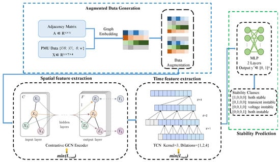
Figure 1. The framework of the joint STCGCN stability prediction.

The STCGCN architecture combines contrastive graph representation learning with temporal feature extraction, as illustrated in Figure 1. Let $\mathbf{X}\in {\mathbb{R}}^{N\times T\times d}$ denote the PMU input tensor for N buses, T time steps, and d features.

2.1. Supervised Contrastive GCN Encoder

The contrastive GCN learns spatial topological representations by aggregating localized neighborhoods across all nodes and time steps [23]. Given an undirected graph $\mathcal{G}=(\mathcal{V},\mathcal{E})$ with adjacency matrix $\mathbf{A}\in {\mathbb{R}}^{N\times N}$ and input tensor $\mathbf{X}\in {\mathbb{R}}^{T\times N\times d}$ (T time steps, N buses, and d features per bus), the spatial dependencies are processed at each time step [23]:

$${\mathbf{H}}_t^{(l+1)}=ReLU\left({\tilde{\mathbf{D}}}^{-{\displaystyle \frac{1}{2}}}\tilde{\mathbf{A}}{\tilde{\mathbf{D}}}^{-{\displaystyle \frac{1}{2}}}{\mathbf{H}}_t^{\left(l\right)}{\Theta }^{\left(l\right)}\right)\mathrm{for}t=1,\dots ,T$$

(1)

where ${\mathbf{H}}_t^{\left(0\right)}=\mathbf{X}{[t,:,:]}^{\top }\in {\mathbb{R}}^{N\times d}$ is the feature matrix at time t, $\tilde{\mathbf{A}}=\mathbf{A}+{\mathbf{I}}_N$ adds self-connections, and $\tilde{\mathbf{D}}$ is the degree matrix of $\tilde{\mathbf{A}}$ with ${\tilde{D}}_{ii}={\sum }_j{\tilde{A}}_{ij}$.

This implements spatiotemporal Laplacian smoothing, where each node’s representation becomes a weighted average of its neighbors and itself at each time step. After the final layer L, node features are aggregated to obtain a global temporal representation:

$${\mathbf{h}}_t={\displaystyle \frac{1}{N}}\sum _{i=1}^N{\mathbf{H}}_t^{\left(L\right)}[i,:]\in {\mathbb{R}}^{d_{\mathrm{gcn}}}$$

(2)

The sequence of global representations forms the output:

$$\mathbf{H}={\left[{\mathbf{h}}_1,{\mathbf{h}}_2,\dots ,{\mathbf{h}}_T\right]}^{\top }\in {\mathbb{R}}^{T\times d_{\mathrm{gcn}}}$$

(3)

In contrastive learning, sample relationships are defined through positive and negative pairs, which jointly determine the structure of the learned representation space. In terms of stability class, a positive pair consists of two samples that share the same joint stability class label, regardless of differences in their underlying topologies or operating conditions. Negative pairs refer to any pair of samples with different joint stability labels that are treated as negative pairs. At the same time, the power grid topology is encoded using contrastive GCN for feature representation.

The supervised contrastive loss ${\mathcal{L}}_{\mathrm{cont}}$ operates on the entire sequence representation [24]:

$${\mathcal{L}}_{\mathrm{cont}}=\sum _{i\in I}{\displaystyle \frac{-1}{\left|P\right(i\left)\right|}}\sum _{p\in P\left(i\right)}log{\displaystyle \frac{exp(s({\mathbf{H}}^{\left(i\right)},{\mathbf{H}}^{\left(p\right)})/\tau )}{{\sum }_{j\in S\left(i\right)}exp(s({\mathbf{H}}^{\left(i\right)},{\mathbf{H}}^{\left(j\right)})/\tau )}}$$

(4)

where $I=\{1,\dots ,2B\}$ is the index set of augmented samples in batch size B, $P\left(i\right)=\{p\in I\setminus \left\{i\right\}\mid y_p=y_i\}$ is the positive set the sample with the same joint stability class label, $S\left(i\right)=I\setminus \left\{i\right\}$ is the comparison set, $s({\mathbf{H}}^{\left(i\right)},{\mathbf{H}}^{\left(j\right)})={\displaystyle \frac{⟨\mathrm{vec}\left({\mathbf{H}}^{\left(i\right)}\right),\mathrm{vec}\left({\mathbf{H}}^{\left(j\right)}\right)⟩}{\parallel \mathrm{vec}\left({\mathbf{H}}^{\left(i\right)}\right)\parallel \parallel \mathrm{vec}\left({\mathbf{H}}^{\left(j\right)}\right)\parallel }}$ is the normalized sequence similarity, and $\tau >0$ is the temperature parameter. The formulation applies supervised contrastive learning by utilizing label-derived relationships, treating all same-class sequences as positives. The supervised contrastive loss is computed over anchor i, with the positive set $P\left(i\right)$ containing all samples that share anchor i’s label (excluding i itself). The loss function simultaneously pulls $(i,p)$ pairs for $p\in P\left(i\right)$ closer together while pushing away representations from different classes.

2.2. Temporal Convolutional Network

The Temporal Convolutional Network (TCN) extracts temporal features from the global system dynamics. The TCN takes as input the global temporal representation $\mathbf{H}\in {\mathbb{R}}^{T\times d_{\mathrm{gcn}}}$ generated by the contrastive GCN, where $\mathbf{H}=f_{\theta }(\mathbf{A},\mathbf{X})$ is obtained through spatial aggregation over all nodes (Section 2.1), T is the number of time steps, and $d_{\mathrm{gcn}}$ is the spatial feature dimension. It is worth noting that our fusion is strictly sequential rather than branched. The GCN-derived H encapsulates not only nodal states but also graph-induced relational context, making it a topology-infused temporal input. The TCN processes the global sequence using stacked dilated causal convolutions. The output at position t in layer l is computed as

$${\mathbf{Z}}_t^{\left(l\right)}=\sum _{k=0}^{K-1}{\mathbf{W}}_k^{\left(l\right)}{\mathbf{h}}_{t-k·{\delta }^{\left(l\right)}}^{(l-1)}+{\mathbf{b}}^{\left(l\right)}$$

(5)

where ${\mathbf{Z}}_t^{\left(l\right)}\in {\mathbb{R}}^{d_{\mathrm{out}}^{\left(l\right)}}$ is the output feature at time t and layer l, K denotes the convolution kernel size, ${\delta }^{\left(l\right)}$ represents the dilation factor at layer l (${\delta }^{\left(l\right)}=2^{l-1}$ for $l\ge 1$), ${\mathbf{W}}_k^{\left(l\right)}\in {\mathbb{R}}^{d_{\mathrm{in}}^{\left(l\right)}\times d_{\mathrm{out}}^{\left(l\right)}}$ are learnable filters ($d_{\mathrm{in}}^{\left(1\right)}=d_{\mathrm{gcn}}$), ${\mathbf{b}}^{\left(l\right)}\in {\mathbb{R}}^{d_{\mathrm{out}}^{\left(l\right)}}$ is the bias term, and ${\mathbf{h}}^{\left(0\right)}=\mathbf{H}$ is the input sequence

The causal constraint prevents future information leakage:

$${\mathbf{h}}_{t-k·{\delta }^{\left(l\right)}}^{(l-1)}=\mathbf{0}\mathrm{for}t-k·{\delta }^{\left(l\right)}<0$$

(6)

Dilated convolutions enable exponential receptive field growth. For L layers with kernel size K:

$$R=1+(K-1)·\sum _{l=1}^L{\delta }^{\left(l\right)}=1+(K-1)(2^L-1)$$

(7)

Residual blocks with skip connections mitigate gradient vanishing as follows:

$${\mathbf{h}}^{\left(l\right)}=ReLU\left(\mathcal{F}\left({\mathbf{h}}^{(l-1)}\right)\right)+\mathcal{H}\left({\mathbf{h}}^{(l-1)}\right)$$

(8)

where $\mathcal{F}$ denotes convolution operations, and $\mathcal{H}$ is a 1×1 convolution for dimension matching.

The final TCN output $\mathbf{Z}\in {\mathbb{R}}^{d_{\mathrm{tcn}}\times d_{\mathrm{gcn}}}$ is obtained through temporal aggregation, where $d_{\mathrm{tcn}}$ is the temporal feature dimension (number of output channels), and $d_{\mathrm{gcn}}$ is preserved as the spatial feature dimension. This matrix $\mathbf{Z}$ contains compressed spatiotemporal features of the entire system and serves as input to the MLP classifier for global stability prediction.

2.3. MLP Classifier for Stability Prediction

The MLP classifier receives the global temporal feature matrix $\mathbf{Z}\in {\mathbb{R}}^{d_{\mathrm{tcn}}\times d_{\mathrm{gcn}}}$ from the TCN output, where $d_{\mathrm{tcn}}$ is the TCN output temporal feature dimension and $d_{\mathrm{gcn}}$ is the GCN output spatial feature dimension. The input to the MLP is prepared by flattening the feature matrix into a vector:

$$\mathbf{z}=\mathrm{vec}\left(\mathbf{Z}\right)\in {\mathbb{R}}^{d_{\mathrm{tcn}}·d_{\mathrm{gcn}}}$$

(9)

The MLP architecture processes this global representation to produce the final stability prediction:

• Input Layer: Receives the flattened feature vector $\mathbf{z}\in {\mathbb{R}}^{d_{\mathrm{in}}}$ where $d_{\mathrm{in}}=d_{\mathrm{tcn}}·d_{\mathrm{gcn}}$.
• Hidden Layers: Each hidden layer applies an affine transformation followed by ReLU activation:

  $${\mathbf{u}}^{\left(k\right)}=ReLU\left({\mathbf{\Phi }}^{\left(k\right)}{\mathbf{u}}^{(k-1)}+{\mathit{\beta }}^{\left(k\right)}\right)$$

  (10)

  where ${\mathbf{u}}^{\left(0\right)}=\mathbf{z}$, ${\mathbf{\Phi }}^{\left(k\right)}\in {\mathbb{R}}^{d_k\times d_{k-1}}$ is the weight matrix, and ${\mathit{\beta }}^{\left(k\right)}\in {\mathbb{R}}^{d_k}$ is the bias vector.
• Output Layer: Produces logits for the system-wide stability prediction:

  $$\widehat{\mathbf{y}}={\mathbf{\Phi }}^{\left(K\right)}{\mathbf{u}}^{(K-1)}+{\mathit{\beta }}^{\left(K\right)}$$

  (11)

  where K is the total number of layers. The output dimension $d_K=4$ corresponds to the four stability classes defined in Equation (14).

The predicted probability vector for the entire system is obtained via softmax:

$$p^{\left(c\right)}={\displaystyle \frac{exp\left({\widehat{y}}^{\left(c\right)}\right)}{{\sum }_{k=1}^{4}exp\left({\widehat{y}}^{\left(k\right)}\right)}},c=1,2,3,4$$

(12)

where $p^{\left(c\right)}$ represents the probability that the power system belongs to stability class c.

2.4. Spatiotemporal Joint Training and Loss Functions

The joint training strategy is presented in Algorithm 1:

The parameters in the training procedure are associated with the supervised contrastive and joint-task cross-entropy loss functions ${\mathcal{L}}_{\mathrm{cont}}$ and ${\mathcal{L}}_{\mathrm{task}}$. The joint training utilizes supervised contrastive loss function ${\mathcal{L}}_{\mathrm{cont}}$ for representation learning as follows:

$${\mathcal{L}}_{\mathrm{cont}}=\sum _{i\in I}{\displaystyle \frac{-1}{\left|P\right(i\left)\right|}}\sum _{p\in P\left(i\right)}log{\displaystyle \frac{exp(s({\mathbf{H}}_i,{\mathbf{H}}_p)/\tau )}{{\sum }_{j\in S\left(i\right)}exp(s({\mathbf{H}}_i,{\mathbf{H}}_j)/\tau )}}$$

(13)

where I is the set of indices for all augmented samples in a batch, $P\left(i\right)$ is the set of indices of positive samples sharing the same stability label $y_i$, $S\left(i\right)=I\setminus \left\{i\right\}$ is the comparison set, $s({\mathbf{H}}_i,{\mathbf{H}}_j)={\displaystyle \frac{⟨\mathrm{vec}\left({\mathbf{H}}_i\right),\mathrm{vec}\left({\mathbf{H}}_j\right)⟩}{\parallel \mathrm{vec}\left({\mathbf{H}}_i\right)\parallel \parallel \mathrm{vec}\left({\mathbf{H}}_j\right)\parallel }}$ computes cosine similarity between flattened sequence representations, $\tau >0$ is the temperature hyperparameter, and ${\mathbf{H}}_i\in {\mathbb{R}}^{T\times d_{\mathrm{gcn}}}$ is the global temporal representation for sample i. Under supervised contrastive learning, the model maps samples from the same stability class to nearby points in the embedding space while pushing apart samples from different classes. Because positive pairs are constructed across heterogeneous network topologies, the objective explicitly promotes invariance to structural variations, thereby enhancing generalization to previously unseen topologies.

The GCN mapping function $f_{\theta }$ generates global temporal representations:

$${\mathbf{H}}_{\mathrm{gcn}}=f_{\theta }(\mathbf{A},\mathbf{X})={\left[{\displaystyle \frac{1}{N}}\sum _{n=1}^N{\mathrm{GCN}}^{\left(L\right)}(\mathbf{A},{\mathbf{X}}_t)\right]}_{t=1}^T\in {\mathbb{R}}^{T\times d_{\mathrm{gcn}}}$$

(14)

where $\mathbf{X}\in {\mathbb{R}}^{N\times T\times d}$ is the PMU measurement tensor, $\mathbf{A}\in {\mathbb{R}}^{N\times N}$ is the topology-adaptive adjacency matrix, and ${\mathrm{GCN}}^{\left(L\right)}$ denotes the final GCN layer output. The adjacency matrix $\mathbf{A}$ is dynamically constructed using grid-informed electrical parameters:

$$A_{ij}=\left\{\begin{array}{cc}{K}_{ij}sin({\delta }_i-{\delta }_j)\hfill & (i,j)\in {\mathcal{E}}_p^{\mathrm{norm}}\hfill \\ 0\hfill & \mathrm{otherwise}\hfill \end{array}\right.$$

(15)

After pretraining and freezing ${\theta }^{*}$, the joint task cross entropy loss function ${\mathcal{L}}_{\mathrm{task}}$ is defined as

$${\mathcal{L}}_{\mathrm{task}}=-\sum _{c=1}^4{y}_{c}log\left({\widehat{y}}_c\right)$$

(16)

where $y_c$ is the ground truth stability label for class c (system-level), and ${\widehat{y}}_c$ is the predicted probability for class c (system-level). The prediction vector $\widehat{\mathbf{y}}\in {\mathbb{R}}^4$ represents system-wide stability probabilities:   

$$\widehat{\mathbf{y}}=f_{\varphi }\left(\mathbf{Z}\right)=\sigma \left({\mathbf{\Phi }}^{\left(2\right)}\left[ReLU\left({\mathbf{\Phi }}^{\left(1\right)}\mathrm{vec}\left(\mathbf{Z}\right)+{\mathit{\beta }}^{\left(1\right)}\right)\right]+{\mathit{\beta }}^{\left(2\right)}\right)$$

(17)

where $\mathbf{Z}=f_w\left({\mathbf{H}}_{\mathrm{gcn}}\right)\in {\mathbb{R}}^{d_{\mathrm{tcn}}\times d_{\mathrm{gcn}}}$ is the global feature matrix, $\mathrm{vec}\left(\mathbf{Z}\right)$ flattens the matrix to ${\mathbb{R}}^{d_{\mathrm{tcn}}·d_{\mathrm{gcn}}}$, and $\sigma \left(·\right)$ is the softmax activation.

3. Dataset Generation with Topology Variation

3.1. PMU Data Generation with Topology Variation

To emulate a realistic wide-area monitoring system (WAMS) and ensure observability of critical dynamics, PMUs are assumed to be installed at all generator buses and a subset of critical load buses. In the IEEE 39-bus system, this corresponds to PMUs placed at the 10 generator buses (Buses 30–39), which directly capture the rotor-angle and frequency dynamics of synchronous machines. In addition, PMUs are installed at several key load buses selected based on electrical centrality, e.g., Buses 4, 8, 15, 16, 20, and 21, to enhance spatial coverage of the network. This configuration ensures that all input features, including voltage magnitude $\left|U\right|$, and relative phase $U_{\theta }$, are consistently derived from these designated PMU locations.

The dataset generation framework presented in Algorithm 2 is used for the IEEE N-bus system through three-level stochastic perturbations.

$$\mathcal{D}=\bigcup _{i=1}^{N_{\mathrm{topo}}}\bigcup _{j=1}^{N_{\mathrm{load}}}\bigcup _{k=1}^{N_{\mathrm{fault}}}\mathrm{Sim}({\mathcal{G}}_i,P_{L,j},{\varphi }_k)$$

(18)

where $N_{\mathrm{topo}}$: number of topology variants, $N_{\mathrm{load}}$: loading conditions, and $N_{\mathrm{fault}}=\left|\mathcal{E}\right|$: branch fault locations. Given the setup, one topology instance ${\mathcal{G}}_i=(\mathcal{V},{\mathcal{E}}_i)$ is generated via the Markov chain edge replacement algorithm.

For each graph topology instance ${\mathcal{G}}_i$, the loading profile matrix is generated, as follows:

$${\mathbf{P}}_L={\mathbf{P}}_{L0}\odot (1+\Delta \mathbf{M})$$

(19)

where $\Delta \sim \mathcal{U}(-0.1,0.1)$ and $\mathbf{M}\in {\{0,1\}}^{N\times T}$ masks variation application nodes. The inputs to the proposed joint prediction framework are the feature matrix of transient dynamic time series data $\mathbf{X}=\{{\mathbf{x}}_{\mathbf{1}},{\mathbf{x}}_{\mathbf{2}},\cdots ,{\mathbf{x}}_{\mathbf{F}}\}\in {\mathbb{R}}^{F\times N\times l}$:

$${\mathbf{x}}_{\mathbf{i}}={\left[\begin{array}{cccc}PM{U}_1^i\left(0\right)& PM{U}_2^i\left(0\right)& \dots & PM{U}_N^i\left(0\right)\\ PM{U}_1^i\left(1\right)& PM{U}_2^i\left(1\right)& \dots & PM{U}_N^i\left(1\right)\\ ⋮& ⋮& ⋮& ⋮\\ PM{U}_1^i(l-1)& PM{U}_2^i(l-1)& \dots & PM{U}_N^i(l-1)\end{array}\right]}^T$$

(20)

where $i=1,2,\dots ,F$, F denotes the number of features, and N represents the number of nodes. The $j^{th}$ column of ${\mathbf{x}}_{\mathbf{i}}$ constitutes the post-fault time series of length l, describing one PMU data stream $PM{U}_j^i$ at node j ($j=1,2,\dots ,N$) in power systems. Consequently, the bus relative phase ($U_{\theta }$), bus voltage magnitude ($\left|U\right|$), rotor angles ($\theta$), and rotor speed ($\omega$) are selected as features for the input $\mathbf{X}=\{U_{\theta },|U|,\theta ,\omega \}$, where $F=4$.

3.2. Stability Labeling

Transient stability is determined by the transient stability index (TSI) ${\sigma }_{TSI}$ [25]:

$${\sigma }_{TSI}={\displaystyle \frac{180-|\Delta {\delta }_{ij}{|}_{max}}{180+|\Delta {\delta }_{ij}{|}_{max}}}$$

(21)

where $|\Delta {\delta }_{ij}{|}_{max}$ denotes the maximum absolute value of rotor angle difference between any two synchronous machines during simulation. The label $y_T$ is defined by the sign of ${\sigma }_{TSI}$:

$$\begin{array}{c}\hfill y_T=\left\{\begin{array}{cc}0& {\sigma }_{TSI}>0\\ 1& {\sigma }_{TSI}⩽0\end{array}\right.\end{array}$$

(22)

The voltage stability label $y_V$ determines whether the voltage magnitude dip/sag of any bus in the system exceeds 20% for more than 50 cycles [26], defined as

$$y_{\mathrm{V}}=\left\{\begin{array}{cc}1\hfill & \mathrm{if}\underset{t}{min}{V}_{\mathrm{limit}}\left(t\right)>0.8\mathrm{p}.\mathrm{u}.\hfill \\ 0\hfill & \mathrm{otherwise}\hfill \end{array}\right.$$

(23)

where $V_{\mathrm{limit}}$ represents the minimum voltage limit.

As presented in Table 1, the stability label $y_c$ for the STCGCN model training is a one-hot encoded variable for the four classes:

$$\left\{\right[1,0,0,0],[0,1,0,0],[0,0,1,0],[0,0,0,1\left]\right\},$$

determined by the transient stability label $y_T$ and voltage stability label $y_V$.

Table 1. Description as table header, please confirm. of label $y_T$ and $y_V$ as one-hot form for transient stability and voltage stability.

Label y	${\mathit{y}}_{\mathit{T}}$ = 1	${\mathit{y}}_{\mathit{T}}$ = 0
$y_V$ = 1	[1, 0, 0, 0]	[0, 1, 0, 0]
$y_V$ = 0	[0, 0, 1, 0]	[0, 0, 0, 1]

4. Results and Discussion

The proposed STCGCN model is validated on the IEEE 39-bus system using time-domain simulations implemented in the Power System Toolbox (PST). Each simulation spans $10\mathrm{s}$ with a time step of $0.01\mathrm{s}$ (i.e., $100\mathrm{Hz}$ sampling), comprising $1\mathrm{s}$ of pre-fault evolution and $9\mathrm{s}$ of post-fault response. Numerical integration employs the trapezoidal method with a tolerance of ${10}^{-6}$ per unit.

Fault scenarios are generated by applying a balanced three-phase short circuit at $t=0.10\mathrm{s}$, cleared at $t=0.1667\mathrm{s}$ (four cycles at $60\mathrm{Hz}$). Load levels are varied by scaling active power uniformly to 90–$110\%$ of the base case while maintaining a constant reactive power factor. To reflect uncertainty, zero-mean Gaussian perturbations are superimposed with a standard deviation of $\pm 5\%$ of the base active-power level. For each of the 20 topology configurations considered, each of the 46 transmission branches is faulted in turn. Every $(\mathrm{topology},\mathrm{faulted}\mathrm{branch})$ pair is repeated 25 times with independent load/noise realizations, yielding a dataset of $20\times 46\times 25=23,000$ labeled samples.

The joint stability assessment is cast as a binary classification for transient stability and voltage stability (stable vs. unstable), using the conventional confusion-matrix definitions. Unstable operating states are labeled as the positive class; stable states are labeled as the negative class. Let $TP$, $TN$, $FP$, and $FN$ denote true positives, true negatives, false positives, and false negatives, respectively. Accuracy (ACC), False Negative Rate (FNR), and False Positive Rate (FPR) are reported and defined as

$$\mathrm{ACC}={\displaystyle \frac{TP+TN}{TP+TN+FP+FN}},\mathrm{FNR}={\displaystyle \frac{FN}{TP+FN}},\mathrm{FPR}={\displaystyle \frac{FP}{FP+TN}}.$$

(24)

ACC reflects overall correctness. FNR quantifies missed detections of instability critical for safety-critical operation. FPR measures false alarms, which affect operator burden and automated protection logic.

4.1. Dataset Construction and Splits

Twenty varied power systems are synthesized with distinct topologies using Algorithm 2. These are partitioned into disjoint sets: fourteen topologies for training, two for validation, and four for testing. Two regimes are evaluated as follows: (i) in-sample, where test events come from topologies that also appear in the training split (but are held out as distinct events); and (ii) out-of-sample, where test events arise from topologies unseen during training. All models are first trained on 20,700 labeled events and then evaluated on 2300 held-out topological loading scenarios drawn from the same topology family (in-sample) without reusing any training events. The joint STCGCN model is trained on the dataset. The optimal hyperparameters for STCGCN are summarized in Table 2. A grid search strategy was employed to identify these optimal hyperparameters.

Table 2. Hyperparameter settings and selection rationale for the STCGCN model.

Category	Hyperparameter	Value	Selection Criteria
Architecture	GCN Layers	3	Balances spatial feature extraction depth and computational cost. Fewer layers led to underfitting, while more caused overfitting.
	GCN Hidden Dimension	256	Provides sufficient model capacity. Determined via grid search over {128, 256, 512}.
	TCN Kernel Size	3	Effective for capturing local temporal patterns.
	TCN Dilation Rates	{1, 2, 4}	Designed to capture multi-scale electromechanical dynamics within the 0.4 s window.
	Dropout Rate	0.2	Mitigates overfitting; validated on the out-of-sample topology test set.
	MLP Hidden Units	512	Offers ample nonlinear transformation capability for the final joint classification.
Training	Batch Size	64	Maximizes GPU memory utilization while maintaining stable gradient descent.
	Initial Learning Rate	$1\times {10}^{-3}$	Used with the Adam optimizer for stable and efficient convergence.
SCL	Temperature ($\tau$)	0.1	Scales the cosine similarity in the contrastive loss function.
	Projection Head Dim	128	Projects GCN embeddings into the space where contrastive loss is applied.
	Positive Pair Margin	0.5	Defines the similarity threshold for constructing positive pairs in SCL.
Data	Observation Window	0.40 s	Selected as the optimal trade-off between prediction accuracy and real-time latency, as analyzed in Section 4.5.

The supervised contrastive learning objective requires the construction of positive sample pairs, generated via a physics-informed data augmentation process. For each input graph-sequence sample ${\mathbf{x}}_i$ in a batch, an augmented view ${\tilde{\mathbf{x}}}_i$ is generated by applying stochastic perturbations hat reflect realistic power system variations while preserving the original stability label $y_i$. Specifically, three augmentation strategies are employed as follows: injecting Gaussian noise into raw PMU measurements to emulate sensor errors; applying minor topology perturbations, such as randomly switching the status of a single branch, under the constraint that the resulting system retains the same stability class, thereby explicitly enforcing topology-invariant representations; and perturbing load profiles within ±5% to capture normal operating condition fluctuations.

4.2. Training Procedure and Representation Quality

Training proceeds in two stages. First, a supervised contrastive GCN encoder is optimized to map PMU time-series samples into a feature space where intra-class pairs are tightly clustered and inter-class pairs are well separated. Figure 2 shows the training loss trajectories. To visualize GCN feature clustering segregation, high-dimensional embeddings are projected to 2D UMAP [27], and Figure 3 shows clear separation among stable vs. unstable events, and between voltage-unstable and transient-unstable subsets. As shown in Figure 3, samples belonging to the same stability category form tight clusters in the latent space, indicating that the model indeed learns topology-invariant feature representations. The cluster segregation indicates that supervised contrastive GCN learning yields discriminative, class-aware representations that provide a strong basis for the downstream TCN and MLP classifier. The generalization is examined by applying the supervised contrastive GCN encoder to out-of-sample events from the power systems with grid topologies never seen during training. As shown in Figure 4, the contrastive GCN feature embeddings preserve cluster structure despite topology changes, evidencing robust cross-topology feature segregation.

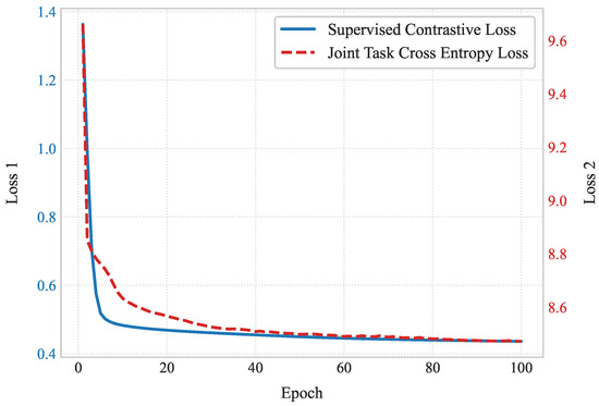
Figure 2. Training loss curves for the joint prediction model.

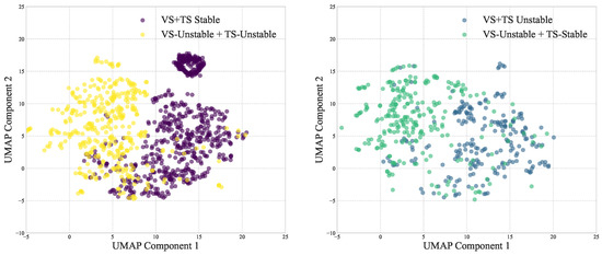
Figure 3. In-sample dataset GCN encoder representation quality. Two-dimensional UMAP projection of supervised contrastive GCN features showing clear cluster separation among stable, unstable, voltage-unstable, and transient-unstable feature labels.

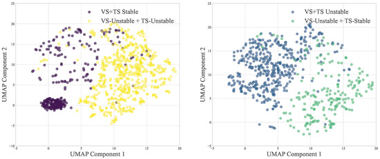
Figure 4. Out-of-sample dataset GCN encoder representation quality. Two-dimensional UMAP projection of supervised contrastive GCN features obtained with the out-of-sample with unseen topologies, showing clear cluster separation and demonstrating cross-topology robustness.

4.3. Classification Benchmark

The confusion matrices are reported for both regimes, the in-sample and out-of-sample datasets. Figure 5 shows the confusion matrix of the STCGCN model on the in-sample test dataset with topologies during training, and accuracy is 89.66%. Figure 6 shows the confusion matrix of the STCGCN model on the out-of-sample test dataset with the unseen topologies during training, and accuracy is 87.73%. In addition, Table 3 and Table 4 show the recall and F1-Score of STCGCN evaluated on the in-sample and out-of-sample datasets.

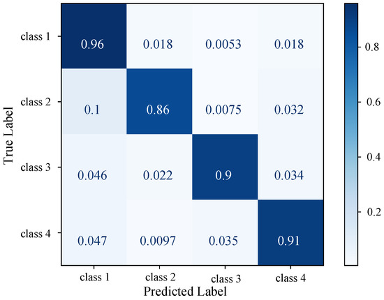
Figure 5. STCGCN confusion matrix on the in-sample dataset. Four classes (class 1, class 2, class 3, and class 4) correspond to one-hot labels $[1,0,0,0]$, $[0,1,0,0]$, $[0,0,1,0]$, and $[0,0,0,1]$, respectively.

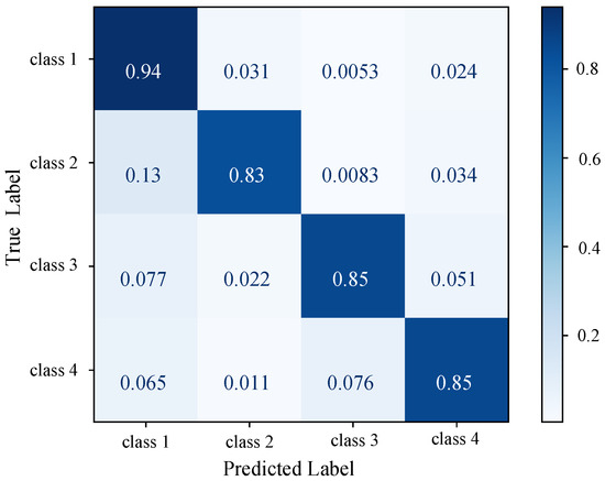
Figure 6. STCGCN confusion matrix on the out-of-sample dataset. Four classes (class 1, class 2, class 3, and class 4) correspond to one-hot labels $[1,0,0,0]$, $[0,1,0,0]$, $[0,0,1,0]$, and $[0,0,0,1]$, respectively.

Table 3. Per-class performance metrics of STCGCN on in-sample dataset.

Class	Precision	Recall	F1-Score	Support
Class 1	0.889	0.959	0.923	1690
Class 2	0.948	0.858	0.901	1203
Class 3	0.934	0.899	0.916	785
Class 4	0.896	0.908	0.902	925

Table 4. Per-class performance metrics of STCGCN on the out-of-sample dataset.

Class	Precision	Recall	F1-Score	Support
Class 1	0.853	0.941	0.871	1690
Class 2	0.942	0.842	0.865	1178
Class 3	0.874	0.861	0.868	782
Class 4	0.869	0.847	0.856	945

While performance decreases slightly under topology shift, accuracy remains high, indicating that the model adapts to structural changes and sustains effective stability prediction.

To quantify the advantages of the proposed contrastive learning-based joint task (STCGCN) prediction model, the Spatiotemporal Embedding Graph Neural Network (STEGNN) [14] is used as the spatiotemporal baseline for comparison. The STEGNN architecture comprises (i) a multi-head supervised contrastive GCN for topological feature extraction, (ii) a TCN for temporal dynamics, and (iii) an MLP classifier. Training uses standard cross-entropy loss.

Figure 7 presents the confusion matrix of STEGNN on the in-sample test set (seen topologies), and Figure 8 shows the corresponding results on the out-of-sample test set (unseen topologies). Table 5 and Table 6 report accuracy and sample counts for STEGNN and STCGCN on both settings. On the out-of-sample set, STCGCN attains 87.73% accuracy versus 79.00% for STEGNN, an absolute gain of 8.73 percentage points, corresponding to 402 additional correct classifications out of 4600 samples. The improvement comes from the topology-aware representation learning induced by the supervised contrastive objective, which enhances cross-topology feature separability, and to the joint (multi-task) formulation that exploits the coupling between voltage and transient stability.

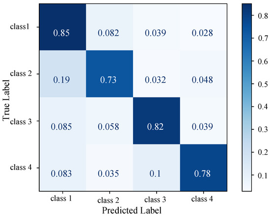
Figure 7. STEGNN confusion matrix on the in-sample test dataset with unseen topologies. Four classes (class 1, class 2, class 3, and class 4) correspond to one-hot labels $[1,0,0,0]$, $[0,1,0,0]$, $[0,0,1,0]$, and $[0,0,0,1]$.

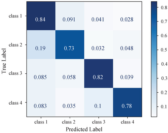
Figure 8. STEGNN Confusion matrix on the out-of-sample test dataset with unseen topologies. Four classes (class 1, class 2, class 3, and class 4) correspond to one-hot labels $[1,0,0,0]$, $[0,1,0,0]$, $[0,0,1,0]$, and $[0,0,0,1]$.

Table 5. Performance of STCGCN vs. STEGNN in the out-of-sample dataset with unseen power grid topologies.

Method	Correct	Missing	Accuracy (%)
STCGCN	4036	564	87.73
STEGNN	3746	854	81.43

Table 6. Performance of STCGCN vs. STEGNN in the in-sample dataset with unseen power grid topologies.

Method	Correct	Missing	Accuracy (%)
STCGCN	4124	476	89.66
STEGNN	3634	966	79.00

To rigorously evaluate the reliability of the STCGCN method, experiments were repeated over three independent runs with different random seeds for model initialization and data shuffling. The mean accuracy and corresponding standard deviation are reported in Table 7 for the in-sample and out-of-sample datasets.

Table 7. Performance and result reliability.

Model	In-Sample Dataset (%)	Out-of-Sample Dataset (%)
STCGCN (Run 1)	89.51	87.62
STCGCN (Run 2)	90.12	88.05
STCGCN (Run 3)	89.08	86.91
STCGCN (Mean ± SD)	$89.66\pm 0.85$	$87.73\pm 1.02$

4.4. Joint-Task and Single-Task Prediction

The joint-task STCGCN prediction is further compared against the single-task prediction that estimates only transient stability (TSP) or only voltage stability (VSP). As shown in Table 8 and Table 9, the joint STCGCN improves both heads: TSP accuracy rises from single-task 86.60% to joint-task 90.34%, and VSP accuracy from 82.56% to 94.63%. These gains reflect the benefits of joint-task learning, where shared spatiotemporal representations and supervised contrastive alignment leverage the physical coupling between voltage and angle dynamics.

Table 8. Transient stability prediction (TSP): single-task vs. joint-task for the IEEE 39-bus system.

Method	Correct	Missing	Accuracy (%)
Single-task TSP	3984	616	86.60
Joint-task TSP	4156	444	90.34

Table 9. Voltage stability prediction (VSP): single-task vs. joint-task for the IEEE 39-bus system.

Method	Correct	Missing	Accuracy (%)
Single-task VSP	3798	802	82.56
Joint-task VSP	4353	247	94.63

4.5. Impact of Observation Window Length

The effect of the post-fault observation window length on prediction accuracy is evaluated, aiming to maximize accuracy while minimizing latency. Using the same hyperparameters as in Table 2, the performance is assessed for multiple PMU window lengths after fault clearing, increasing the window in 0.05 s increments. Figure 9 plots test accuracy versus window length; the corresponding performance metrics are listed in Table 10. Accuracy plateaus for windows of about 0.40 s and longer: the joint STCGcN model attains 87.73% at 0.40 s and 87.91% at 0.45 s (with no meaningful gains beyond). Therefore, 0.40 s is selected as a practical trade-off between real-time responsiveness and accuracy.

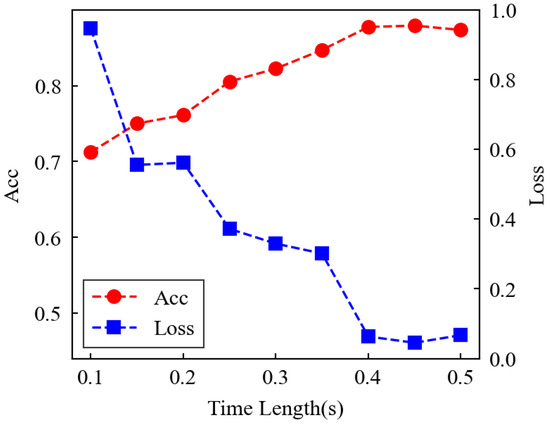
Figure 9. Effect of post-fault PMU window length on the joint STCGCN prediction accuracy in the IEEE 39-bus system.

Table 10. Performance comparison across different window sizes.

	Window (s)
	0.10	0.15	0.20	0.25	0.30	0.35	0.40	0.45	0.50
Joint-task in four classes
ACC (%)	71.24	75.01	76.12	80.54	82.24	84.71	87.73	87.91	87.34
Joint-task TSP
ACC (%)	74.32	77.85	79.08	83.67	85.42	88.13	90.34	90.28	89.97
FPR (%)	10.87	9.42	8.65	7.34	6.73	6.28	6.06	6.11	6.09
FNR (%)	24.25	21.50	19.15	16.84	14.92	14.08	13.82	13.91	13.87
Joint-task VSP
ACC (%)	78.95	82.43	84.17	88.92	90.86	92.98	94.63	94.57	94.21
FPR (%)	6.15	5.48	4.87	4.13	3.78	3.52	3.45	3.48	3.46
FNR (%)	15.43	13.62	11.95	9.84	8.92	8.67	8.61	8.65	8.69

The practical deployability of STCGCN is assessed by benchmarking inference latency on a system with an AMD EPYC 7763 (64-core) CPU and an NVIDIA GeForce RTX 4090 GPU, using PyTorch 1.9.0 with CUDA 11.1. Experiments were run on 10,000 randomly selected test samples. Table 11 reports the average per-sample inference time for multiple batch sizes, a metric that is critical for real-time deployment where end-to-end latency typically must remain below 50 ms per prediction. STCGCN attains a single-sample inference latency of 18.5 ms, well below the 50 ms real-time threshold, and achieves a batched throughput of approximately 3265 samples/s. These results indicate ample headroom for real-time deployment, enabling sub-second stability assessment even under large-scale power grids.

Table 11. Inference time for STCGCN on the IEEE 39-bus system.

Batch Size	Avg. Time (ms)	Throughput (Samples/s)
1	18.5	54.1
8	12.3	650.4
32	9.8	3265.3

4.6. Sensitivity to PMU Noise

The analyses above assumed lossless PMU delivery [28]. In practice, PMU measurements exhibit noise with typical standard deviations in the range $0.0005$–$0.01$ p.u. [29] and signal-to-noise ratios (SNR) around 45 dB. The robustness is evaluated by injecting Gaussian noise at different SNR levels and reporting ACC, FNR, and FPR for both tasks. Results in Table 12 show that performance degrades gradually as SNR declines; degradation remains modest above 40dB and becomes more pronounced below this threshold, yet overall accuracy stays comparatively high—indicating strong noise robustness of STCGCN. On the IEEE 39-bus system, the joint-task STCGCN model achieves 87.73 accuracy on the out-of-sample dataset with the unseen topologies, outperforming the STEGNN baseline (79.00%) by +8.73 percentage points, and exhibiting superior generalization under $N-1$ contingencies and topology changes.

Table 12. Joint-task STCGCN performance under different PMU SNR levels in the IEEE 39-bus system.

Task	SNR (dB)	Metrics
		ACC (%)	FNR (%)	FPR (%)
Joint-task TSP	None	90.34	13.82	6.06
	60	89.97	14.25	6.38
	50	89.23	14.88	6.92
	40	87.85	16.24	7.81
	30	84.06	19.83	10.52
	20	80.37	23.14	13.75
Joint-task VSP	None	94.63	8.61	3.45
	60	94.25	8.92	3.78
	50	93.68	9.47	4.25
	40	92.31	10.85	5.14
	30	88.92	14.24	8.03
	20	85.43	17.86	11.32

5. Conclusions

Modern power systems, driven by high renewable penetration and frequent topology reconfigurations, require precise and rapid stability assessments to ensure reliable operation. The STCGCN model is proposed for the joint prediction of voltage and transient stability. The architecture integrates a graph-convolutional encoder to model spatial and topological dependencies, coupled with a temporal–convolutional network to capture fast electromechanical dynamics. This design enables an accurate representation of coupled voltage and transient stability dynamics. To maintain resilience under switching operations, STCGCN applies a topology-adaptive adjacency matrix in the contrastive GCN learning using real-time electrical features, including line admittance, impedance, power-flow magnitudes, and directions. Furthermore, it employs a class-weighted loss function and physics-informed data augmentation to mitigate class imbalance and enhance feature discrimination across diverse operating conditions, such as load and renewable fluctuations.

On the IEEE 39-bus system, STCGCN achieves 87.73% accuracy for joint stability prediction on a test set with unseen topologies, outperforming the STEGNN baseline’s 79.00% accuracy. Compared to the single-task models, the joint-task STCGCN model significantly enhances performance for both voltage stability prediction (94.63% vs. 82.56%) and transient stability prediction (90.34% vs. 86.60%). These results demonstrate the value of the joint-task STCGCN model. The model achieves stable accuracy with only 0.40 s of post-fault data, supporting real-time contingency screening. It also exhibits resilience under N–1 contingencies and topology variations. Noise-stress tests confirm consistent performance for PMU signal-to-noise ratios (SNR) ≥ 40 dB, ensuring practical deployability in noisy environments.

STCGCN redefines real-time power system stability assessment by addressing three critical challenges: the decoupled modeling of voltage and transient stability, reliance on static topology assumptions, and class imbalance. By integrating spatial, temporal, and task-coupled dynamics, it enables robust and scalable stability prediction, paving the way for the secure operation of renewable-rich grids. Future research will scale STCGCN to larger systems, such as the IEEE 118-bus grid, incorporate cyber–physical constraints like cyberattack resilience, and optimize for edge deployment to support ultra-fast, decentralized stability control. These advancements will drive the adoption of data-driven solutions for next-generation power systems, ensuring resilience and efficiency in dynamic grid environments. The STCGCN framework, with its demonstrated ability to learn topology-invariant representations, opens avenues for applications in broader cyber-physical power-energy systems. For example, the GCN naturally models the physical connectivity of charging stations and the logical communication links in a unified manner.

References

- Olanrewaju, R.; Thanasingh, M.J.C.; Al-Greer, M. Techno-Economic Evaluation of Hybrid Renewable Energy Systems for Power Supply. In Proceedings of the 2024 29th International Conference on Automation and Computing (ICAC), Sunderland, UK, 28–30 August 2024; pp. 1–6. [Google Scholar] [CrossRef]
- Wang, D.; Jiang, Y.; Qiu, C.; Xiong, H.; Bi, M.; Ge, Y.; Li, J.; Cao, Y.; Li, G.; Cui, Z.; et al. Power System Real Time Reliability Monitoring and Security Assessment in Short-term and on-line Mode. In Proceedings of the 2019 IEEE Innovative Smart Grid Technologies—Asia (ISGT Asia), Chengdu, China, 21–24 May 2019; pp. 758–763. [Google Scholar] [CrossRef]
- Kundur, P.; Paserba, J.; Ajjarapu, V.; Andersson, G.; Bose, A.; Canizares, C.; Hatziargyriou, N.; Hill, D.; Stankovic, A.; Taylor, C.; et al. Definition and classification of power system stability IEEE/CIGRE joint task force on stability terms and definitions. IEEE Trans. Power Syst. 2004, 19, 1387–1401. [Google Scholar] [CrossRef]
- Wang, H.; Li, Z. A Review of Power System Transient Stability Analysis and Assessment. In Proceedings of the 2019 Prognostics and System Health Management Conference (PHM-Qingdao), Qingdao, China, 25–27 October 2019; pp. 1–6. [Google Scholar] [CrossRef]
- ALShamli, Y.; Hosseinzadeh, N.; Yousef, H.; Al-Hinai, A. A review of concepts in power system stability. In Proceedings of the 2015 IEEE 8th GCC Conference & Exhibition, Muscat, Oman, 1–4 February 2015; pp. 1–6. [Google Scholar] [CrossRef]
- Li, X.; Li, Z.; Guan, L.; Zhu, L.; Liu, F. Review on Transient Voltage Stability of Power System. In Proceedings of the 2020 IEEE Sustainable Power and Energy Conference (iSPEC), Chengdu, China, 23–25 November 2020; pp. 940–947. [Google Scholar] [CrossRef]
- Hatziargyriou, N.; Milanovic, J.; Rahmann, C.; Ajjarapu, V.; Canizares, C.; Erlich, I.; Hill, D.; Hiskens, I.; Kamwa, I.; Pal, B.; et al. Definition and Classification of Power System Stability—Revisited & Extended. IEEE Trans. Power Syst. 2021, 36, 3271–3281. [Google Scholar] [CrossRef]
- Dehghani, M.; Ghiasi, M.; Niknam, T.; Rouzbehi, K.; Wang, Z.; Siano, P.; Alhelou, H.H. Control of LPV Modeled AC-Microgrid Based on Mixed H2/H∞ Time-Varying Linear State Feedback and Robust Predictive Algorithm. IEEE Access 2022, 10, 3738–3755. [Google Scholar] [CrossRef]
- Sun, Y.; Li, X.; Yan, S.; Song, Y.; Farsangi, M. Novel decentralized robust excitation control for power system stability improvement. In Proceedings of the International Conference on Electric Utility Deregulation and Restructuring and Power Technologies, London, UK, 4–7 April 2000; pp. 443–448. [Google Scholar] [CrossRef]
- Ishimaru, M.; Yokoyama, R.; Shirai, G.; Lee, K. Allocation and design of robust TCSC controllers based on power system stability index. In Proceedings of the 2002 IEEE Power Engineering Society Winter Meeting, New York, NY, USA, 27–31 January 2002; Volume 1, pp. 573–578. [Google Scholar] [CrossRef]
- Lei, B.; Wu, X.; Fei, S. Nonlinear robust control design for SSSC to improve damping oscillations and transient stability of power system. In Proceedings of the 2017 36th Chinese Control Conference (CCC), Dalian, China, 26–28 July 2017; pp. 3101–3106. [Google Scholar] [CrossRef]
- Löper, M.; Trummal, T.; Kilter, J. Analysis of the Applicability of PMU Measurements for Power Quality Assessment. In Proceedings of the 2018 IEEE PES Innovative Smart Grid Technologies Conference Europe (ISGT-Europe), Sarajevo, Bosnia and Herzegovina, 21–25 October 2018; pp. 1–6. [Google Scholar] [CrossRef]
- Sun, P.; Huo, L.; Chen, X.; Liang, S. Rotor Angle Stability Prediction Using Temporal and Topological Embedding Deep Neural Network Based on Grid-Informed Adjacency Matrix. J. Mod. Power Syst. Clean Energy 2024, 12, 695–706. [Google Scholar] [CrossRef]
- Deng, C.; Dai, L.; Chao, W.; Huang, J.; Wang, J.; Lin, L.; Qin, W.; Lai, S.; Chen, X. An Advanced Spatio-Temporal Graph Neural Network Framework for the Concurrent Prediction of Transient and Voltage Stability. Energies 2025, 18, 672. [Google Scholar] [CrossRef]
- Alimi, O.A.; Ouahada, K.; Abu-Mahfouz, A.M. A Review of Machine Learning Approaches to Power System Security and Stability. IEEE Access 2020, 8, 113512–113531. [Google Scholar] [CrossRef]
- Zhou, Y.; Xu, T.; Ye, L.; Liu, M.; Chen, X.; Yang, Y.; Guo, Q.; Sun, H. Transient Rotor Angle and Voltage Stability Discrimination Based on Deep Convolutional Neural Network with Multiple Inputs. In Proceedings of the 2021 IEEE 4th International Electrical and Energy Conference (CIEEC), Wuhan, China, 28–30 May 2021; pp. 1–6. [Google Scholar] [CrossRef]
- Hu, Y.; Yang, X.; Gu, W.; Lang, Y.; Wu, X.; Yu, Y. Identification of Power Angle Instability and Transient Voltage Instability Based on Deep Learning. In Proceedings of the 2019 IEEE 3rd Conference on Energy Internet and Energy System Integration (EI2), Changsha, China, 8–10 November 2019; pp. 759–764. [Google Scholar] [CrossRef]
- Thukaram, D.; Khincha, H.; Ravikumar, B. A New Approach for Fault Location Identification in Transmission system using Stability Analysis and SVMs. In Proceedings of the 2006 International Conference on Power Electronic, Drives and Energy Systems, New Delhi, India, 12–15 December 2006; pp. 1–6. [Google Scholar] [CrossRef]
- Plathottam, S.J.; Salehfar, H.; Ranganathan, P. Convolutional Neural Networks (CNNs) for power system big data analysis. In Proceedings of the 2017 North American Power Symposium (NAPS), Morgantown, WV, USA, 17–19 September 2017; pp. 1–6. [Google Scholar] [CrossRef]
- Hossain, R.R.; Huang, Q.; Huang, R. Graph Convolutional Network-Based Topology Embedded Deep Reinforcement Learning for Voltage Stability Control. IEEE Trans. Power Syst. 2021, 36, 4848–4851. [Google Scholar] [CrossRef]
- Hossain, R.; Gautam, M.; MansourLakouraj, M.; Livani, H.; Benidris, M. Voltage Control in Distribution Grids Using Topology Aware Deep Reinforcement Learning. In Proceedings of the 2023 IEEE Industry Applications Society Annual Meeting (IAS), Nashville, TN, USA, 29 October–2 November 2023; pp. 1–7. [Google Scholar] [CrossRef]
- Deng, Y.; Lin, S.; Jia, H.; Tong, X. Optimal allocation of voltage sag meters with power system topology variation considered. In Proceedings of the 2022 China Automation Congress (CAC), Xiamen, China, 25–27 November 2022; pp. 3145–3150. [Google Scholar] [CrossRef]
- Kipf, T.N.; Welling, M. Semi-Supervised Classification with Graph Convolutional Networks. arXiv 2017, arXiv:cs.LG/1609.02907. [Google Scholar] [CrossRef]
- Khosla, P.; Teterwak, P.; Wang, C.; Sarna, A.; Tian, Y.; Isola, P.; Maschinot, A.; Liu, C.; Krishnan, D. Supervised Contrastive Learning. arXiv 2021, arXiv:cs.LG/2004.11362. [Google Scholar] [PubMed]
- Ye, X.; Morales, J.D.; Milanović, J.V. Truncated Transient Stability Index for On-line Power System Transient Stability Assessment. In Proceedings of the 2021 IEEE PES Innovative Smart Grid Technologies Europe (ISGT Europe), Espoo, Finland, 18–21 October 2021; pp. 1–5. [Google Scholar] [CrossRef]
- He, Q.; Qi, F.; Wang, S.; Zeng, Y.; Sheng, H.; Ma, J. Research on Static Voltage Stability Index of Regional Power Network with New Energy Stations Based on Voltage Stability Criterion. In Proceedings of the 2023 IEEE 7th Conference on Energy Internet and Energy System Integration (EI2), Hangzhou, China, 15–18 December 2023; pp. 2597–2601. [Google Scholar] [CrossRef]
- Li, B.; Zheng, Y.; Ran, R. 2DUMAP: Two-Dimensional Uniform Manifold Approximation and Projection for Fault Diagnosis. IEEE Access 2025, 13, 12819–12831. [Google Scholar] [CrossRef]
- Rafique, Z.; Khalid, H.M.; Muyeen, S.; Kamwa, I. Bibliographic review on power system oscillations damping: An era of conventional grids and renewable energy integration. Int. J. Electr. Power Energy Syst. 2022, 136, 107556. [Google Scholar] [CrossRef]
- Okendo, E.O.; Wekesa, C.W.; Saulo, M.J. Optimal placement of Phasor Measurement Unit considering System Observability Redundancy Index: Case study of the Kenya power transmission network. Heliyon 2021, 7, e07670. [Google Scholar] [CrossRef] [PubMed]
Disclaimer/Publisher’s Note: The statements, opinions and data contained in all publications are solely those of the individual author(s) and contributor(s) and not of MDPI and/or the editor(s). MDPI and/or the editor(s) disclaim responsibility for any injury to people or property resulting from any ideas, methods, instructions or products referred to in the content. |
© 2025 by the authors. Licensee MDPI, Basel, Switzerland. This article is an open access article distributed under the terms and conditions of the Creative Commons Attribution (CC BY) license (https://creativecommons.org/licenses/by/4.0/).