Abstract
Large-scale wind power grid-connected systems can trigger the risk of power system instability. In order to enhance the stability margin of grid-connected systems, this paper accurately characterizes the topology of the global boundary of stability domain (BSD) of the grid-connected system based on BSD theory, using the method of combining the manifold topologies and singularities at infinity. On this basis, the effect of large-scale doubly fed induction generators (DFIGs) replacing synchronous units on the BSD of the system is analyzed. Simulation results based on the IEEE 39-bus system indicate that the negative impedance characteristics and low inertia of DFIGs lead to a contraction of the stability domain. The principle of singularity invariance (PSI) proposed in this paper can effectively expand the BSD by adjusting the inertia and damping, thereby increasing the critical clearing time by about 5.16% and decreasing the dynamic response time by about 6.22% (inertia increases by about 5.56%). PSI is superior and applicable compared to traditional energy functions, and can be used to study the power angle stability of power systems with a high proportion of renewable energy.
1. Introduction
Under the global initiative to achieve the dual carbon goals, the proportion of renewable energy in power systems has been steadily increasing. Wind power, as a crucial renewable energy source, has witnessed large-scale integration, becoming a key trend in the power industry development [1]. However, the extensive integration of wind power introduces significant challenges to grid stability, substantially increasing the risk of instability. Traditional power systems, supported by synchronous generators, exhibit strong inertia and stability. Nevertheless, large-scale wind power integration alters the power supply structure, where the widespread adoption of the doubly fed induction generator (DFIG) reduces system inertia and significantly diminishes regulation capability under disturbances, making the system more prone to instability and seriously threatening the secure and reliable operation of power systems [2]. The transient power angle stability of a wind power system refers to the ability of the system to maintain synchronous operation and return to a stable equilibrium state after the power grid suffers a major disturbance (such as a short-circuit fault or generator disconnection) [3]. The measurement standards for transient power angle stability typically include indicators such as critical clearing time (CCT) and dynamic response performance [4].
To effectively enhance the stability margin of wind power grid-connected systems, researchers have conducted extensive studies. Existing research methods primarily encompass time-domain simulation, direct methods, and hybrid approaches. Some scholars have used time-domain simulation to numerically solve the differential-algebraic equations, which can more accurately simulate the dynamic response of the system, but the computational complexity is high when dealing with large-scale wind power clusters. The method in [5] has the advantage of efficiently evaluating the nonlinear stability and analyzing the parameter sensitivity by combining the time-reversal trajectory, but it is limited to the model simplification that may ignore the high-frequency dynamics. In [6], the case of a real weak grid was employed to verify the damping performance of DFIG. It fails to take into account the effect of wind speed fluctuation. The approach in [7] has the advantage of quantifying the effect of uncertainty factors on the stability by using a probabilistic method to avoid the conservative design, which has a high computational burden and relies on a stand-alone equivalent model. Among the direct methods, perturbation function and manifold topology are the most typical. Some scholars have directly quantified the effect of perturbations on the stability domain of the system based on the perturbation function. Reference [8] proposed the oscillatory energy transfer-based control of grid-configured wind turbines, which effectively coordinates the design contradiction between virtual inertia and virtual damping, and significantly improves the stability of the grid, with the limitation that the control effect depends on the exact synchronous torque coefficient parameter. Reference [9] proposed the stochastic transient energy function method based on the structural retention model, which models the load stochastic perturbation as a Wiener process, and reveals the amplitude of the fluctuation and geographic distribution on the stability law, but the reliance on Monte Carlo simulation leads to low computational efficiency. Reference [10] proposed a hybrid method of a linear Lyapunov function and inverse time trajectory to estimate the transient stability boundary of a wind turbine converter, which reduces the computational volume significantly. The accuracy of the inverse trajectory is affected by the quality of the initial value of the linear Lyapunov function. A deeper understanding of the behavior of the system on long-term time scales, especially how the stochasticity brought by renewable energy sources such as wind power affects the global dynamic structure of the system, requires a re-examination of the stability of the system from the perspective of the manifold topology. The theory of manifolds provides a powerful tool for analyzing the geometrical structure of coupled systems at multiple time scales, and is capable of downscaling high-dimensional stochastic dynamical systems to key invariant manifolds, thus revealing the essential features of their long-term evolution. Reference [11] proposed a deterministic model-based approach for long-term stability analysis of power systems by means of manifold topology and singular uptake theory, which accurately approximates the effects of stochastic wind power while ensuring the computational efficiency. It is limited by the assumption of the stability of the slow manifolds and the simplified treatment of the discrete events. Reference [12] constructed a multiparameter practical stable manifold for wind power grid-connected systems through limit ring tracking and bifurcation theory, with the advantage of accurately portraying the stability boundary of the nonlinear system and quantifying the effect of time lag on the contraction of the stable manifold. The parameter uncertainty and the complex perturbation of the high-dimensional manifold topology due to the multiple time-lag coupling were not taken into account.
To precisely quantify the impact of wind power integration on system stability and improve stability margins, this paper proposes a global boundary of stability domain (BSD) characterization method that integrates manifold topology analysis with the singularities at infinity (SAIs), overcoming the limitations of traditional local stability analysis. The main contributions of this work include the following:
- Equivalent Model of DFIG: By analyzing the dynamic behavior of DFIGs during faults and their impact on the power grid, a simplified equivalent model for grid-connected DFIGs is established.
- Precise BSD Characterization via Manifold–Singularity Synergy: Through analyzing the stable/unstable manifold topological structures near system equilibrium points and incorporating SAIs to characterize nonlinear behaviors under extreme conditions, high-precision BSD computation is achieved, providing new insights for stability analysis of wind power grid-connected systems.
- Quantitative Mechanism of DFIG’s Impact on Stability Domain: By studying the BSD topology, the relationship between DFIG penetration rate and stability margins is revealed, elucidating the dynamic mechanism of stability domain contraction under high wind power penetration.
- Transient Stability Enhancement via Principle of Singularity Invariance (PSI): A transient stability principle based on preserving the topological characteristics of SAIs is proposed, demonstrating stability margin improvement through parameter regulation in the practical IEEE 39-bus system. The comparative study of transient stability margin enhancement in this paper is through a comparison based on the specific physical mechanisms of singularity invariance and energy function invariance. This is significantly different from the current mainstream cutting-edge methods (e.g., data-driven transient stability rapid assessment based on transient stability [13,14], AI-assisted optimal control strategies [15,16], etc.) in terms of theoretical foundation, modeling assumptions, optimization goals, and application focus. While the existing frontier methods mainly focus on rapid identification of destabilization modes or data-based prediction of control boundaries, the core of this study is to reveal the intrinsic constraints on stability margins imposed by a specific physical mechanism and to derive a direct principle. Therefore, at this stage, directly comparing the quantitative performance of the results of this study with these methods with different theoretical foundations under a unified standard may make it difficult to fairly evaluate their respective advantageous features. As it is well known that extensive comparisons for verifying innovativeness and generalizability are important, these will be the key directions for the future in-depth development of this study.
2. Modeling of the Wind Power Grid-Connected System and Its Global BSD Topology Characterization
2.1. Dynamic Characteristics of DFIG
The doubly fed induction generator (DFIG) exhibits significantly different dynamic characteristics from traditional synchronous generators during power system transient processes. To facilitate the analysis of the DFIG’s dynamic behavior during faults and its impact on the power grid, it can be simplified using the Thevenin’s equivalent circuit [17,18,19,20].
The stator voltage equation can be expressed as:
where is the stator voltage. and are the stator and rotor currents, respectively. and are the stator and rotor magnetic flux linkages, respectively. and are the stator and rotor resistances, respectively. is the synchronous angular velocity. and are the stator and rotor self inductances, respectively. is the mutual inductance between the stator and rotor. To simplify the analysis, we define the following:
- Transient reactance:
- Internal voltage:
The stator current term is , which is a fixed value. Note that is related to by:
Here, and represent the equivalent internal resistance and transient reactance of the DFIG converter, respectively. The equivalent circuit of the DFIG is illustrated in Figure 1.
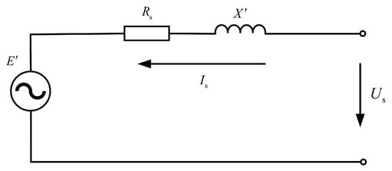
Figure 1.
DFIG internal equivalent circuit.
During fault conditions, of the DFIG dynamically adjusts with the changes in stator and rotor flux linkages, resulting in nonlinear external characteristics. Based on the DFIG’s power characteristics, and during faults can be expressed as:
where represents the voltage phase angle at the point of grid connection of the DFIG and s denotes the slip ratio. represents the active power of the DFIG, and represents the reactive power of the DFIG.
The relationship between and is expressed as . Combining this relationship with Equation (6), the equivalent resistance is derived as:
Similarly, the equivalent reactance is obtained as:
These results demonstrate that the DFIG behaves as a negative impedance [21,22] during fault conditions, whose magnitude is closely related to and . Therefore, the DFIG’s equivalent negative impedance can be expressed as:
2.2. Multi-Machine System Dimensionality Reduction
In the multi-machine system modeling of this paper, to simplify the analysis process, the dynamic response of the excitation system and speed control system are both ignored, and it is assumed that the load is equivalent to the impedance and included in the node admittance matrix. Assuming the system consists of n generators, the rotor phase angle and angular velocity of each generator jointly constitute the dynamic state variables of the system. The generators interact with each other through the power flow coupling relationship of the power grid, thereby forming a nonlinear differential equation system with a dimension of . This system not only has a high dimension but also exhibits strong coupling and nonlinear relationships among its state variables, leading to challenges such as high computational complexity and difficulty in directly characterizing the BSD when conducting transient stability domain analysis, singularity tracking, and manifold computation. Therefore, to reduce the system dimension, this paper introduces the equivalent modeling and dimensionality reduction process as shown in Figure 2. First, based on the trend of the power angle curve changes in the post-fault system, the multi-machine system is divided into critical machine groups (S group) and non-critical machine groups (A group) using the single-machine equivalent (SIME) [23] method. Next, using the inertia center theory [24,25], the mathematical models of the two groups of systems can be further processed to obtain a two-machine system. Finally, a relative power angle is established between the two machines to characterize their relative motion, simplifying the system into a one-machine infinite bus system (OMIB) containing only two variables, namely and .
The SIME method is briefly described as follows.

Figure 2.
Dimensionality reduction process.
The center-of-angle for each group is defined as:
where and represent the equivalent inertia for each group, respectively.
Assuming the two machine groups have different damping, and , the dynamic equations can be derived as:
where and denote mechanical power inputs, while and represent electromagnetic power outputs.
Further simplification of gives:
Assuming an equivalent damping:
The system dynamics can be described by:
where , , and . Assuming no power angle oscillations within each group, the electromagnetic powers are expressed as:
Substituting and simplifying yields:
where , , and . Defining and , we obtain the final equivalent equation:
Through the DFIG equivalence and multi-machine system reduction process described above, the complex multi-machine system is simplified to an OMIB. For analytical convenience, let us define ; then, the OMIB equation can be expressed as:
where represents relative angular velocity, , , , and . Building upon this foundation, we proceed with modeling and analyzing the DFIG, with particular focus on the electromagnetic power parameters. Figure 3 shows the equivalent circuit of the entire grid-connected system after incorporating the DFIG equivalence from Section 2.1.
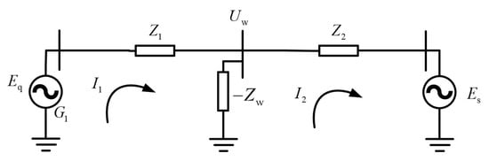
Figure 3.
Equivalent circuit of the wind power grid-connected system.
Considering the DFIG integration, the loop current equations can be formulated based on Figure 3, yielding the expression for loop current :
where and represent the self impedance and mutual impedance, respectively. They are defined as:
where and represent the self-impedance angle and mutual impedance angle, respectively. Combining Equations (22) and (23), we can derive the electromagnetic power angle equation for the grid-connected system as shown in Equation (25).
2.3. The Local Manifold Topology
System (22) possesses both a stable equilibrium point (SEP) and an unstable equilibrium point (UEP) within the periodic domain . In nonlinear dynamical systems, the stable manifold () and unstable manifold () near the equilibrium points serve as fundamental mathematical tools for characterizing the local manifold topology [13,27]. In the state space, the BSD is composed of the stable manifold of the UEP, whose geometric shape and range constitute the BSD. When disturbances cause the system state to exceed the BSD, the system becomes unstable. Considering the characteristics of DFIGs before and after a fault, this paper equates DFIGs with a negative impedance model after a fault and analyzes them in an equivalent network. This study focuses on the transient power angle stability of wind power grid-connected systems, specifically the ability of the system to maintain stability in the state space and ultimately return to a SEP after suffering severe disturbances.
- For the SEP , the sets of trajectories converging to and diverging from the SEP are, respectively, defined as:
- For the UEP , the corresponding manifolds are:
In power system transient stability analysis, the union of stable manifolds from all Type-I UEPs near Equation (22) constitutes the BSD of the SEP. The stable manifold can be represented by the smooth function:
where and are derived from the left eigenvectors of the Jacobian matrix , with spanning the stable submanifold of the UEP.
As illustrated in Figure 4, the local BSD is characterized by Equation (29). The blue curve represents the BSD. When the stable manifold fails to form a closed domain (the blue curve extends to infinity in Figure 4), the domain becomes unbounded, causing the BSD to expand indefinitely. In such cases, the system behavior at infinity becomes the primary focus of this investigation.
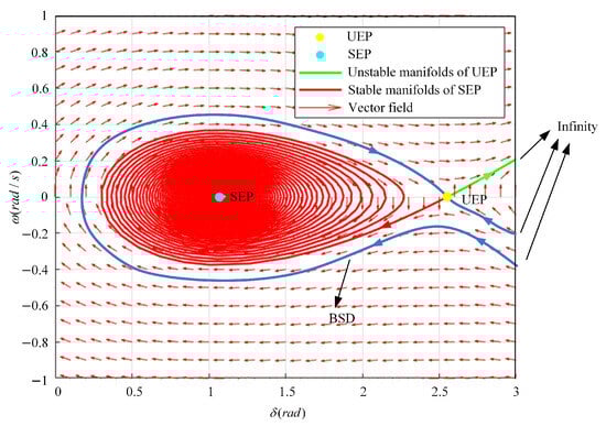
Figure 4.
The local boundary of the stable domain.
2.4. The Global Manifold Topology
While the stable and unstable manifolds of equilibrium points provide crucial local information about nonlinear system dynamics, these local characteristics alone cannot fully reveal the global behavior of the system. To address this limitation, this section introduces a coordinate transformation method that maps the system into a finite space, enabling comprehensive analysis of stability domains and their boundary structures.
Consider the nonlinear dynamical Equation (22). Through an appropriate coordinate transformation, any point in the original state space can be mapped to a corresponding point in the finite space:
As system trajectories approach infinity, they are projected onto a unit sphere in the transformed space:
Considering the neighborhood of as an example, we establish new coordinates with fixed at 1. Figure 5 shows diagram of the coordinate neighborhood near . The geometric relationships show that the line connecting the original system point to the origin intersects both the following surfaces:
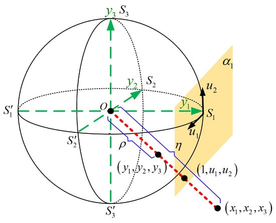
Figure 5.
Diagram of coordinate neighborhood.
- The tangent plane at ;
- The spherical surface at .
These points satisfy the proportional relations:
The coordinate transformation is therefore given by:
Introducing the auxiliary variable and computing partial derivatives yields the differential system:
Solving gives the singularity at infinity (SAI) coordinates on the tangent plane. Combining with the spherical equation , we obtain four SAIs on the sphere, namely , , , and , where the parameters are defined as:
Figure 6 illustrates the distribution of the global BSD and SAIs. As shown in the figure, the global BSD is formed by both the SAIs and the UEPs, which are mapped inside the unit sphere. This geometric representation establishes the foundation for subsequent transient stability analysis.
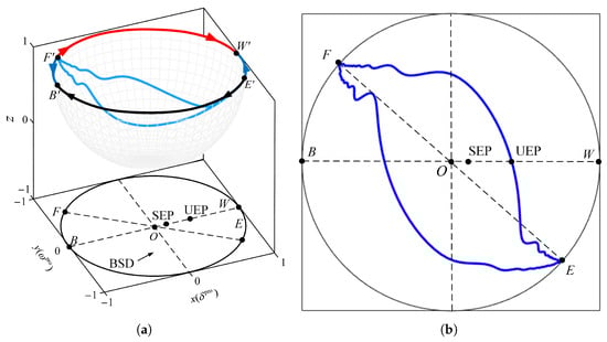
Figure 6.
The distribution of the global BSD and SAIs. (a) The global BSD in the projection space. (b) The distribution of the four SAIs: W, B, E, and F. The blue solid line indicates the BSD.
To visually demonstrate the effect of DFIG penetration replacing synchronous generators (SGs) on the BSD, Figure 7 presents the comparison of the BSD before and after DFIG grid connection, where the black curve represents the original SG-dominated BSD and the blue curve shows the contracted BSD after DFIG integration with displaced SEP and UEPs. This boundary contraction visually confirms the stability-weakening effects of DFIG’s negative impedance characteristics and reduced inertia, while simultaneously validating the effectiveness of the proposed BSD characterization method in capturing these stability domain changes. The results provide clear evidence of how renewable integration alters the fundamental stability properties of power systems.
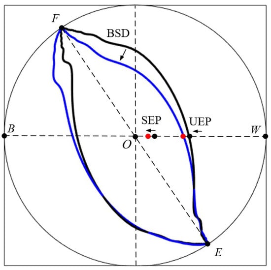
Figure 7.
Comparison of BSD before and after DFIG grid connection.
Furthermore, the results validate the effectiveness of the proposed BSD characterization method in capturing these stability impacts.
2.5. The Principle of Singularity Invariance
The BSDs and SAIs undergo significant changes during grid faults in wind power grid-connected systems. Since Equation (35) reveals that SAIs depend solely on parameters J and , this study proposes a cooperative parameter optimization method to enhance voltage support capability by adjusting J and . Figure 8 illustrates the topological mapping relationships between BSDs and SAIs under three operational states: (1) the pre-fault system (black curve) with stable equilibrium point SEP-0, , unstable equilibrium point UEP-0, , and critical clearing time (CCT), ; (2) the post-fault system (green curve) featuring SEP-1, , UEP-1, , and CCT, ; and (3) the CCT obtained by the adjustment of system parameters following the principle of singularity invariance (PSI), .
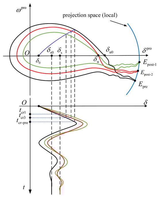
Figure 8.
The variation of the relationship between SAIs and BSDs.
Here, and represent the starting points of BSD manifolds before and after faults, respectively, both mapped in the projection space, while the blue curve demonstrates a sample fault trajectory. The relationship of demonstrates the contraction of the BSD from pre-fault to post-fault conditions. After implementing the PSI regulation, the relationship of confirms BSD expansion, providing theoretical validation of the proposed method’s effectiveness in enhancing system stability.
To enhance post-fault stability through BSD expansion, we implement a system parameter optimization strategy. By analyzing the relationship between , , and the BSD, where , , , and with as initial parameters and as optimized parameters, we observe that BSD expansion causes the downward shift of singularities at infinity. Maintaining BSD consistency requires controlling these singularities to remain fixed (or shift downward), with the necessary and sufficient conditions and , which translates to and .
This leads to the key parameter ratio conservation law:
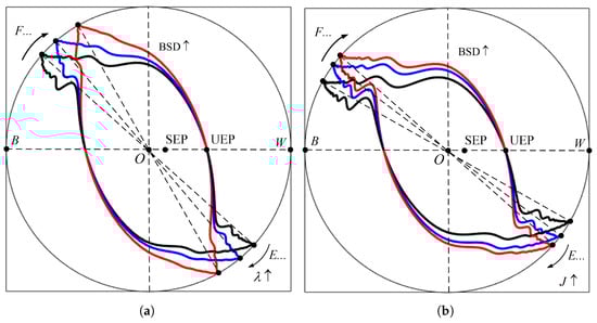
Figure 9.
Relationship between parameter variation and BSDs. (a) Relationship between variation and BSDs. (b) Relationship between J variation and BSDs. The black curve represents the original BSD. The blue curve represents the BSD after the first increase in (increase in J). The red curve represents the BSD after the second increase in (increase in J).
The specific characteristics show that when J or increases, the critical point E shifts downward along the BSD, with the red domain (outer boundary) expansion indicating BSD enlargement. This study confirms that rational parameter configuration can effectively enlarge the stability domain, providing crucial stability control methods for the wind power grid-connected system.
2.6. Restrictive Conditions
For the system model (22) studied above, the damping ratio [28] is expressed as:
where represents synchronous angular frequency. Analysis reveals the following:
- The damping ratio shows positive correlation with damping ()—increasing enhances and accelerates oscillation decay.
- Negative correlation exists with inertia ()—larger J reduces , slowing system response and potentially degrading stability.
Furthermore, both overshoot () and settling time () are governed by the damping ratio:
It is noteworthy that increasing J reduces the system’s natural frequency (), thereby further affecting dynamic response performance. Research indicates that the optimal damping ratio range should be between 0.7 and 1 to balance rapid response with low overshoot characteristics. Specifically, the following apply:
- : faster response but higher overshoot.
- : critically damped with significantly slower response.
3. Simulation Analysis
To validate the effectiveness and accuracy of the proposed method, this section establishes a simulation test environment based on practical power system cases, specifically examining scenarios where wind turbines replace thermal power units with quantitative evaluations performed through CCT and settling time measurements. For comparative analysis, the classical energy function (EF) method serves as the benchmark to highlight the advantages of our method, particularly focusing on the differences in fault critical point identification accuracy and transient stability assessment reliability. All simulations are conducted on the MATLAB/Simulink 2022a platform using the IEEE 39-bus system as the test model, whose typical topology is illustrated in Figure 10.
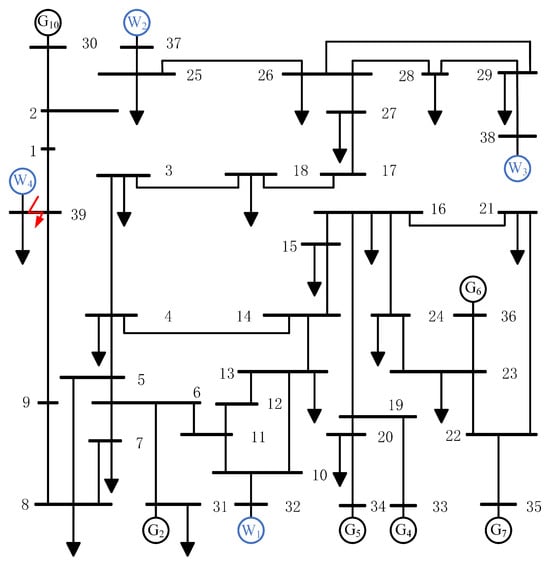
Figure 10.
IEEE 39-bus system.
3.1. Validation of the Proposed Method
To verify the effectiveness of the proposed method, the original system parameters are compared with the regulated system parameters as shown in Table 1, and the comparison between the original BSD and the adjusted BSD is given as shown in Figure 11.

Table 1.
Comparison of the adjusted parameters obtained by the proposed method with the original parameters.
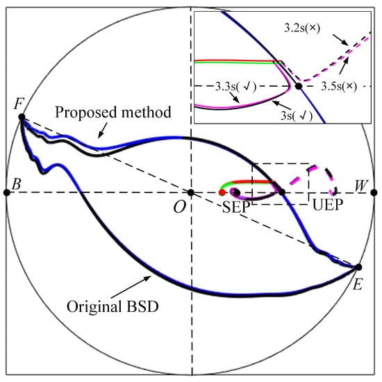
Figure 11.
Comparison of BSD before and after adjustment. “✓” means “stable” after the fault is cleared at that time; “×” means “unstable” after the fault is cleared at that time.
Experimental results demonstrate that the proposed method significantly improves the CCT from the original to , effectively expanding the BSD and enabling the system to tolerate longer fault durations without instability. Specifically, when clearing faults at , the traditional system becomes unstable, while the proposed method maintains stability. When extended to (exceeding the new CCT limit), the expected instability occurs, further validating the BSD expansion effect. Additionally, through optimized system parameters, the proposed method reduces the settling time from to , achieving a 10.3% improvement in dynamic response speed, which indicates faster recovery to steady-state operation and reduced transient stress on equipment. These results confirm that the proposed method not only enhances transient stability but also optimizes dynamic response performance, thereby providing more reliable protection for power system security.
Figure 12 shows that the trajectory of feature root changes during J and changes. The magnitude of J directly affects the sensitivity of the power angle changes. The magnitude of determines the rate at which the oscillations of the system decay. The evolution of the dynamic characteristics as parameters change can be clearly observed in the root locus diagram. As J increases, the system poles move closer to the imaginary axis, and the oscillation frequency of the conjugate complex poles gradually decreases, leading to a slower system response. When J increases from 0.90 to 1.05, the real part of the poles decreases from approximately −0.5 to about −0.4, while the amplitude of the imaginary part correspondingly decreases, indicating that the oscillation characteristics weaken while the inertial effect strengthens. Regarding changes in the damping coefficient , as increases from 0.1 to 10, the system undergoes a typical dynamic characteristic transformation process: In the initial stage (), the poles exhibit distinct conjugate complex characteristics, and the system is in an underdamped state with significant overshoot in the response. When increases to the 1–2 range, the poles gradually move toward the real axis, and the system enters a critically damped state, where the response is both fast and without overshoot. Continuing to increase , the poles eventually split into two real poles, and the system transitions to an overdamped state, where the response speed decreases slightly but stability further improves. By reasonably selecting the combination of J and , the dynamic performance of the system can be precisely controlled.
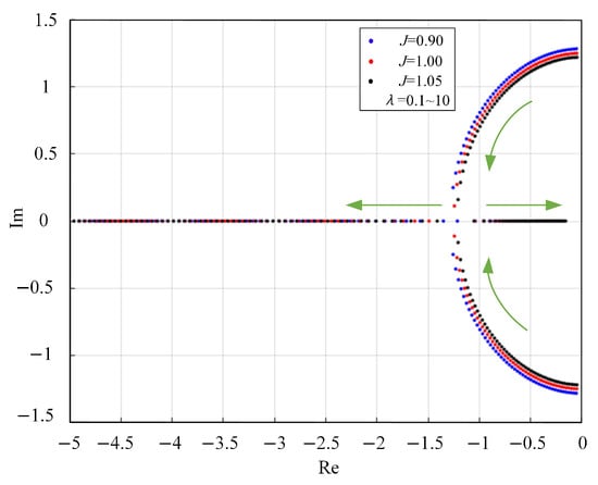
Figure 12.
The trajectory of feature root changes during J and changes. The green arrow indicates the trend of root trajectory changes.
3.2. Validation of the Superiority of the Proposed Method
To validate the superiority of the proposed method, this study compares two methods for maintaining the BSD: the conventional energy function (EF) method that preserves post-fault control energy and the proposed method that maintains SAI invariance. Figure 13 illustrates three distinct BSD curves with their corresponding CCTs and singularity positions. Table 2 shows the comparison of parameter optimization results between the proposed method and the EF method. The subsequent analysis uses and to denote the CCTs achieved by the EF method and the proposed method, respectively, with comparative evaluation of their stability preservation capabilities. The evaluation indices are divided into IDRS% (an evaluation index of dynamic response speed) and ICCT% (an evaluation index of CCT). After the fault occurred, the original conditions of the system were measured as , , s, and s.
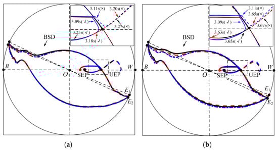
Figure 13.
Comparison of BSD at different parameters obtained by different methods. (a) Comparison of BSD at different J obtained by different methods in terms of Case 1. (b) Comparison of BSD at different obtained by different methods in terms of Case 6. The blue curve represents the original BSD with CCT s and singularity , the red curve shows the EF method BSD associated with singularity , while the black curve demonstrates our method’s BSD-preserving singularity .
Table 2.
Comparison of parameter optimization results between the proposed method and the EF method.
3.2.1. Selection of Different J
In Figure 13a, the CCT obtained by the EF method is , while the proposed method achieves . The relationship of clearly demonstrates that the system regulated by the proposed method exhibits a larger BSD and superior transient stability. This is quantitatively validated in Table 2 (Case 1): when J increases to 0.95 (increasing by about 5.56%), the proposed method achieves ICCT% = 5.16% (indicating that CCT increases by 5.16%) versus 2.90% obtained by the EF method. Similarly, IDRS% = −6.22% (faster dynamic response), which outperforms −3.48% obtained by the EF method. The position of SAIs ( or ) significantly influences the BSD size—when is located below , the red curve becomes larger, indicating better stability than the blue curve. Notably, although the black curve shares the same singularity with the blue curve, its longer CCT proves that our method further enhances stability under identical singularity conditions. In Figure 14a, the dynamic response speed of the two methods is compared using the power angle sequence diagram as the research object, which concludes that the parameters adjusted by the proposed method stabilize faster than the original conditions and the EF method.
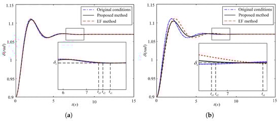
Figure 14.
Comparison of the power angle sequence diagram at different parameters obtained by different methods. (a) Comparison of the power angle sequence diagram at different J obtained by different methods in terms of Case 1. (b) Comparison of the power angle sequence diagram at different obtained by different methods in terms of Case 6. The blue curve, red curve, and black curve represent the power angle sequence diagrams obtained under the original conditions, using the EF method, and using the proposed method, respectively. The corresponding settling times are , , and , respectively.
3.2.2. Selection of Different
In Figure 13b, the EF method yields a CCT of compared to achieved by proposed method, both outperforming obtained by the original condition. The result confirms that the proposed method enables the system to withstand longer fault durations without instability, further improving transient stability. Table 2 (Case 6) quantifies this advantage: when increases to 1.1 (increasing about 10%), the proposed method achieves ICCT% = 18.06% (CCT improvement) versus 17.42% obtained by the EF method, and IDRS% = −17.04% (settling time reduction) versus −16.92% obtained by the EF method. Additionally, in Figure 14b, the proposed method stabilizes the system power angle in a shorter time compared to the EF method.
3.2.3. Overcoming the Conservativeness of the EF Method
First it should be mentioned that the EF method improves the stability of the post-system by enhancing the parameter coordination configuration of the system through a nonlinear function criterion. In contrast, the proposed method in this paper, as derived from Equation (36), improves system stability through a linear function criterion, which is simpler than the EF method. Second, the EF method involves the construction of a relatively complex energy function. Finally, the EF method is limited to models that do not include the randomness of new energy sources, but the proposed method in this paper introduces wind power randomness through the modification of the impedance model.
As shown in Figure 15, the comparison of the three methods—the BSD-stable manifold (red solid line), the EF method (black dashed line), and the proposed method (blue solid line)—demonstrates the superiority of the proposed method. The domain bounded by the red solid line (representing the BSD characterized by manifolds) constitutes the theoretically precise local stability domain. Our method overcomes this limitation by directly analyzing the stable/unstable manifolds of UEPs and SEPs while incorporating singularities at infinity to account for non-local behavior. This is clearly illustrated in Figure 15a,b, where the blue domain encompasses a larger domain than the black domain (as evidenced by ), directly reflecting the capability of the proposed method to expand the BSD while maintaining faster response times.
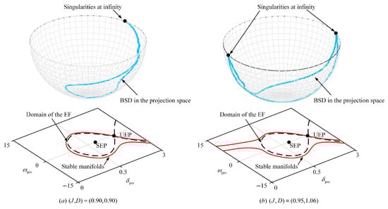
Figure 15.
Comparison of different methods of characterization of BSD. (a) . (b) .
3.3. Sensitivity Analysis
The parameter sensitivity is investigated by fixing the ratio while varying their absolute values. Figure 16 shows the sensitivity of CCT to the parameters obtained by the proposed method.
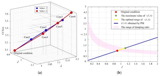
Figure 16.
The sensitivity of CCT to the parameters obtained by the proposed method. (a) The sensitivity of CCT to changes in J or . (b) The optimal range for J and adjustments.
In Figure 16a, adjusting parameters will lead to changes in CCT, that is, changes in BSD. Specifically, although adjusting parameters J or too high will cause the BSD to expand, the damping ratio will exceed the range, resulting in a slower dynamic response speed. Despite these variations, the range of the damping ratio can still be expressed as the pink bandwidth as shown in Figure 16b, indicating that the proposed method needs to be adjusted within the bandwidth. The optimal adjustment range of this experiment is the range marked in yellow in the figure. In practical applications, when adjusting parameters, it is necessary to maintain a sufficient stability margin. The adjustment range should be determined after a fault; that is, when adjusting parameters, it is necessary to ensure both the maximum BSD and the fastest response speed.
4. Discussion
This study provides new theoretical tools and practical guidance for the transient stability analysis of wind power grid-connected systems through an equivalent modeling framework and manifold topology methods. Although the proposed methods perform well under deterministic fault conditions, there are still some issues and future research directions worth further exploration in practical applications.
- (1)
- Addressing the randomness of new energy output: Current research is based on deterministic conditions, while actual wind power output exhibits significant randomness and intermittency. Future research can integrate stochastic dynamic system theory, introduce a Weibull distribution wind speed model, and analyze the dynamic perturbation effects of power fluctuations on the stability domain. Additionally, through stochastic differential equations and Monte Carlo simulations, the stability probability of the system under uncertainty can be quantified, thereby enhancing the robustness and practical applicability of the method.
- (2)
- High-dimensional system expansion: In large test cases with thousands of variables, the proposed method demonstrates good scalability and computational efficiency by combining the manifold topology theory and SAI analysis. Firstly, the high-dimensional multi-machine system is reduced to a low-dimensional nonlinear differential equation by the equivalent model of the DFIG and the dimensionality reduction technique (e.g., the SIME method), and the specific dimensionality reduction process can be referred to in Section 2.2. So as long as the equations of a large test system with thousands of variables are derived, its transient power angle stability can be analyzed using the method of this paper. At this stage, it is not possible to study the performance of the method of this paper in real large-scale test system optimization problems, and we will continue to study it in depth in the future.
- (3)
- Extension to other methods: In existing studies, there are various methods for the transient stability analysis of wind power grid-connected systems, but each of them has certain limitations. In order to more comprehensively assess the advantages and applicability of the method proposed in this paper, Table 3 systematically compares this proposed method with the existing reference methods in terms of the core method, research focus, etc.
Table 3. Differences between the proposed method and existing methods in the field.
Through the comparative analysis, the method of this paper shows unique advantages in theoretical universality and parameter optimization efficiency, which provide new ideas for the stability study of high percentage renewable energy systems. Future work will focus on in-depth exploration in the above directions to further enhance the practicality and robustness of the method.
5. Conclusions
This study successfully characterizes the global BSD of a wind power grid-connected system using manifold theory and the SAI method. Through projective transformations and parameter optimization, we achieve a precise description of the system’s nonlinear dynamics, overcoming the conservativeness of the conventional EF method and providing more accurate theoretical foundations for transient stability analysis.
Three key findings emerge: (1) The replacement of synchronous generators with the DFIG significantly alters system dynamics, manifesting as BSD contraction and CCT reduction. The negative impedance characteristics and low inertia of the DFIG are identified as primary stability-limiting factors, which can be mitigated through coordinated parameter regulation. (2) The proposed PSI, by adjusting key parameters (J, ), effectively expands post-fault BSD while reducing settling time, achieving optimal balance between stability and dynamic response. (3) IEEE 39-bus system simulations validate the method’s effectiveness in enhancing stability for renewable-dominated power systems, providing both theoretical support and practical tools for grid planning and operation.
Author Contributions
Conceptualization, methodology, formal analysis, and writing—original draft preparation, J.Y.; validation, J.Y., M.M., and Y.J.; writing—review and editing, M.M.; supervision, Y.J.; funding acquisition, J.Y. and Y.J. All authors have read and agreed to the published version of the manuscript.
Funding
This work was supported by the Shanghai Sailing Program (Grant No. 22YF1429500) and the Foundation of Key Laboratory of Cleaner Intelligent Control on Coal & Electricity, Ministry of Education, Taiyuan University of Technology (Grant No. CICCE202415).
Data Availability Statement
The original contributions presented in the study are included in the article.
Acknowledgments
The authors gratefully acknowledge the support from the Shanghai Sailing Program (Grant No. 22YF1429500) and the Key Laboratory of Cleaner Intelligent Control on Coal & Electricity, Ministry of Education, Taiyuan University of Technology (Grant No. CICCE202415). We also thank the Department of Electrical Engineering, University of Shanghai for Science and Technology, for providing research facilities and technical support.
Conflicts of Interest
The authors declare no conflicts of interest.
Nomenclature
| Abbreviations | |
| DFIG | Doubly fed induction generator |
| BSD | Boundary of stability domain |
| SEP | Stable equilibrium point |
| UEP | Unstable equilibrium point |
| SAIs | Singularities at infinity |
| OMIB | One-machine infinite bus |
| PSI | Principle of singularity invariance |
| CCT | Critical clearing time |
| EF | Energy function |
| SIME | Single-machine equivalent |
| SG | Synchronous generator |
| 3D | Three-dimensional |
| IDRS% | Evaluation index of dynamic response speed |
| ICCT% | Evaluation index of critical clearing time |
| VSG | Virtual synchronous generator |
| DC | Direct current |
| CPS | Cyber–physical systems |
| Symbols | |
| Stator voltage | |
| Stator current | |
| Rotor current | |
| Stator flux linkage | |
| Rotor flux linkage | |
| Stator resistance | |
| Rotor resistance | |
| Synchronous angular velocity | |
| Stator self inductance | |
| Rotor self inductance | |
| Mutual inductance | |
| Transient reactance | |
| Internal voltage | |
| Voltage phase angle at the point of DFIG grid connection | |
| s | Slip ratio |
| Active power | |
| Reactive power | |
| DFIG equivalent impedance | |
| Impedance between generator G1 and reference node | |
| Impedance between infinite power source and reference node | |
| Self impedance | |
| Self-impedance angle | |
| Mutual impedance | |
| Mutual impedance angle | |
| Equivalent resistance | |
| Equivalent reactance | |
| Excitation voltage | |
| System voltage | |
| Central angle of S group | |
| Central angle of A group | |
| Inertia of S group | |
| Inertia of A group | |
| Self conductance | |
| Mutual susceptance | |
| J | Inertia |
| Damping | |
| The power angle of the i-th generator | |
| The angular velocity of the i-th generator | |
| Relative rotor angle | |
| Relative angular velocity | |
| Total inertia | |
| Equivalent inertia | |
| Equivalent damping | |
| Mechanical power | |
| Electromagnetic power | |
| Reference power | |
| Damping patio | |
| Overshoot | |
| Settling time | |
| Synchronous angular frequency | |
| Natural angular frequency | |
| Critical clearing time | |
| Stable manifold | |
| Unstable manifold | |
| Auxiliary coordinates | |
| Coordinates in the original system | |
| Projected coordinates | |
| State space radius | |
| Projected space radius | |
| Trajectory function | |
| Phase shift angle | |
| SAI coordinate parameters | |
| SAI position functions |
References
- Kim, J.; Bialek, S.; Unel, B.; Dvorkin, Y. Strategic Policymaking for Implementing Renewable Portfolio Standards: A Tri-Level Optimization Approach. IEEE Trans. Power Syst. 2021, 36, 4915–4927. [Google Scholar] [CrossRef]
- Alsmadi, Y.M.; Xu, L.; Blaabjerg, F.; Ortega, A.J.P.; Abdelaziz, A.Y.; Wang, A.; Albataineh, Z. Detailed Investigation and Performance Improvement of the Dynamic Behavior of Grid-Connected DFIG-Based Wind Turbines Under LVRT Conditions. IEEE Trans. Ind. Appl. 2018, 54, 4795–4812. [Google Scholar] [CrossRef]
- Mohammadpour, H.A.; Santi, E. SSR Damping Controller Design and Optimal Placement in Rotor-Side and Grid-Side Converters of Series-Compensated DFIG-Based Wind Farm. IEEE Trans. Sustain. Energy 2015, 6, 388–399. [Google Scholar] [CrossRef]
- Oraa, J.; Samanes, J.; Lopez, J.; Gubia, E. Single-Loop Droop Control Strategy for a Grid-Connected DFIG Wind Turbine. IEEE Trans. Ind. Electron. 2024, 71, 8819–8830. [Google Scholar] [CrossRef]
- Ghosh, S.; Bakhshizadeh, M.K.; Yang, G.; Kocewiak, Ł. An extended nonlinear stability assessment methodology for type-4 wind turbines via time reversal trajectory. CSEE J. Power Energy Syst. 2025, 1–10. [Google Scholar]
- Faried, S.O.; Billinton, R.; Aboreshaid, S. Probabilistic Evaluation of Transient Stability of a Wind Farm. IEEE Trans. Energy Convers. 2009, 24, 733–739. [Google Scholar] [CrossRef]
- Muljadi, E.; Butterfield, C.P.; Parsons, B.; Ellis, A. Effect of Variable Speed Wind Turbine Generator on Stability of a Weak Grid. IEEE Trans. Energy Convers. 2007, 22, 29–36. [Google Scholar] [CrossRef]
- Zhang, X.; Huang, Y.; Fu, Y. Oscillation Energy Transfer and Integrated Stability Control of Grid-Forming Wind Turbines. IEEE Trans. Sustain. Energy 2025, 16, 826–839. [Google Scholar] [CrossRef]
- Bakhshizadeh, M.K.; Ghosh, S.; Yang, G.; Kocewiak, Ł. Transient Stability Analysis of Grid-Connected Converters in Wind Turbine Systems Based on Linear Lyapunov Function and Reverse-Time Trajectory. J. Mod. Power Syst. Clean Energy 2024, 12, 782–790. [Google Scholar] [CrossRef]
- Odun-Ayo, T.; Crow, M.L. Structure-Preserved Power System Transient Stability Using Stochastic Energy Functions. IEEE Trans. Power Syst. 2012, 27, 1450–1458. [Google Scholar] [CrossRef]
- Wang, X.; Chiang, H.-D.; Wang, J.; Liu, H.; Wang, T. Long-Term Stability Analysis of Power Systems with Wind Power Based on Stochastic Differential Equations: Model Development and Foundations. IEEE Trans. Sustain. Energy 2015, 6, 1534–1542. [Google Scholar] [CrossRef]
- Ma, X.; Wan, Y.; Wang, Y.; Dong, X.; Shi, S.; Liang, J.; Zhao, Y.; Mi, H. Multi-Parameter Practical Stability Region Analysis of Wind Power System Based on Limit Cycle Amplitude Tracing. IEEE Trans. Energy Convers. 2023, 38, 2571–2583. [Google Scholar] [CrossRef]
- Wang, T.; Chiang, H.-D. On the Number of System Separations in Electric Power Systems. IEEE Trans. Circuits Syst. I Regul. Pap. 2016, 63, 661–670. [Google Scholar] [CrossRef]
- Qiu, G.; Liu, J.; Liu, Y.; Liu, T.; Mu, G. Ensemble Learning for Power Systems TTC Prediction with Wind Farms. IEEE Access 2019, 7, 16572–16583. [Google Scholar] [CrossRef]
- Jafarzadeh, S.; Genc, I.; Nehorai, A. Real-time transient stability prediction and coherency identification in power systems using Koopman mode analysis. Electr. Power Syst. Res. 2021, 201, 107565. [Google Scholar] [CrossRef]
- Ali, B.M. Deep Reinforcement Learning for Wind-Power: An Overview. In Proceedings of the 2023 6th International Conference on Engineering Technology and its Applications (IICETA), Al-Najaf, Iraq, 15–16 July 2023; pp. 245–251. [Google Scholar]
- Sun, K.; Yao, W.; Fang, J.; Ai, X.; Wen, J.; Cheng, S. Impedance Modeling and Stability Analysis of Grid-Connected DFIG-Based Wind Farm with a VSC-HVDC. IEEE J. Emerg. Sel. Top. Power Electron. 2020, 8, 1375–1390. [Google Scholar] [CrossRef]
- Karaagac, U.; Mahseredjian, J.; Jensen, S.; Gagnon, R.; Fecteau, M.; Kocar, I. Safe Operation of DFIG-Based Wind Parks in Series-Compensated Systems. IEEE Trans. Power Deliv. 2018, 33, 709–718. [Google Scholar] [CrossRef]
- Hu, B.; Nian, H.; Li, M.; Xu, Y.; Liao, Y.; Yang, J. Impedance-Based Analysis and Stability Improvement of DFIG System Within PLL Bandwidth. IEEE Trans. Ind. Electron. 2022, 69, 5803–5814. [Google Scholar] [CrossRef]
- Xiao, Y.T.; Li, G.H.; Wang, W.S.; He, G.Q.; Zhen, N. Oscillation Mechanism Analysis and Suppression Strategy of Renewable Energy Base Connected into LCC-HVDC (Part II): Impedance Characteristics and Oscillation Mechanism Analysis. Proc. CSEE 2024, 44, 4245–4260. [Google Scholar]
- Chen, S.; Yu, S.S.; Zhang, G.; Zhang, Y. Novel VSG Control to Enhance DFIG Oscillatory Stability in Weak Grids via Admittance Modeling: Analysis and Experimental Validation. IEEE Trans. Energy Convers. 2025, 37, 1–13. [Google Scholar] [CrossRef]
- Xing, F.; Xu, Z. Investigation on Negative-Resistance Effect of Doubly-Fed Induction Generator. Acta Energiae Solaris Sin. 2022, 43, 324–332. [Google Scholar]
- Pavella, M.; Ernst, D.; Ruiz-Vega, D. Transient Stability of Power Systems: A Unified Approach to Assessment and Control; Kluwer: Norwell, MA, USA, 2000. [Google Scholar]
- Kuznetsov, Y.A. Elements of Applied Bifurcation Theory, 2nd ed.; Springer: New York, NY, USA, 2004; pp. 40–50. [Google Scholar]
- Si, Y.; Wang, Z.; Liu, L.; Anvari-Moghaddam, A. Impacts of Uncertain Geomagnetic Disturbances on Transient Power Angle Stability of DFIG Integrated Power System. IEEE Trans. Ind. Appl. 2023, 59, 2615–2625. [Google Scholar] [CrossRef]
- Amaral, F.M.; Alberto, F.C. Stability Region Bifurcations of Nonlinear Autonomous Dynamical Systems: Type-Zero Saddle-Node Bifurcations. Int. J. Robust Nonlinear Control 2011, 21, 591–612. [Google Scholar] [CrossRef]
- Meiss, J.D. Differential Dynamical Systems; Society for Industrial and Applied Mathematics: Philadelphia, PA, USA, 2007; pp. 165–186. [Google Scholar]
- Chen, X.; Ma, M.; Yan, Z. An Improved Parameter Boundary Calculation Method for Virtual Synchronous Generator with Capacity Constraints of Energy Storage System. Electr. Power Syst. Res. 2025, 241, 111391. [Google Scholar] [CrossRef]
- Zhuo, Q.; Liu, W.; Xu, Z.; Zhang, H.; Zhai, Y.; Yang, L.; Xu, F. Active Power-Frequency Oscillation Suppression Strategy for Parallel VSG Grid-Connected Power System. In Proceedings of the 2024 10th International Conference on Power Electronics Systems and Applications (PESA), Hong Kong, 5–7 June 2024; pp. 1–6. [Google Scholar]
- Pouresmaeil, M.; Sangrody, R.; Taheri, S.; Montesinos-Miracle, D.; Pouresmaeil, E. Enhancing Fault Ride Through Capability of Grid-Forming Virtual Synchronous Generators Using Model Predictive Control. IEEE J. Emerg. Sel. Top. Ind. Electron. 2024, 5, 1192–1203. [Google Scholar] [CrossRef]
- Li, Y.; Sahoo, S.; Ou, S.; Leng, M.; Vazquez, S.; Dragičević, T.; Blaabjerg, F. Flexible Transient Design-Oriented Model Predictive Control for Power Converters. IEEE Trans. Ind. Electron. 2024, 71, 11377–11387. [Google Scholar] [CrossRef]
- Jongudomkarn, J.; Liu, J.; Ise, T. Virtual Synchronous Generator Control with Reliable Fault Ride-Through Ability: A Solution Based on Finite-Set Model Predictive Control. IEEE J. Emerg. Sel. Top. Power Electron. 2020, 8, 3811–3824. [Google Scholar] [CrossRef]
- Shen, J.; Weng, P.; Shen, Y.; Chen, B.; Yu, L. Distributed Fusion Estimation for Nonlinear Cyber-Physical Systems with Attacked Control Signals. IEEE Syst. J. 2022, 17, 1216–1223. [Google Scholar] [CrossRef]
- Gupta, A.; Sekhar, P.C. Dynamic Droop Control for Optimal Power Sharing in Renewable Rich Hybrid Islanded Microgrids. In Proceedings of the 2024 IEEE International Conference on Power Electronics, Drives and Energy Systems (PEDES), Mangalore, India, 18–21 December 2024; pp. 1–6. [Google Scholar]
- Li, C.; Yang, Y.; Li, Y.; Liu, Y.; Blaabjerg, F. Modeling for Oscillation Propagation With Frequency-Voltage Coupling Effect in Grid-Connected Virtual Synchronous Generator. IEEE Trans. Power Electron. 2025, 40, 82–86. [Google Scholar] [CrossRef]
Disclaimer/Publisher’s Note: The statements, opinions and data contained in all publications are solely those of the individual author(s) and contributor(s) and not of MDPI and/or the editor(s). MDPI and/or the editor(s) disclaim responsibility for any injury to people or property resulting from any ideas, methods, instructions or products referred to in the content. |
© 2025 by the authors. Licensee MDPI, Basel, Switzerland. This article is an open access article distributed under the terms and conditions of the Creative Commons Attribution (CC BY) license (https://creativecommons.org/licenses/by/4.0/).