Fault Location on Three-Terminal Transmission Lines Without Utilizing Line Parameters

Abstract

Transmission lines are constantly exposed to changes in climatic conditions and aging which affect the parameters and change the characteristics of the three-terminal circuit over time. In this paper we propose a fault location algorithm for three-terminal transmission lines to solve this problem. The algorithm utilizes the positive components of the voltage and current signals measured synchronously from the terminals. In this work no prior knowledge of the line parameters was required when calculating the fault location and the use of fault classification algorithms was not necessary. In addition, the proposed method determines the parameters of the line segment and fault location based on a solid mathematical basis and has been verified through simulation results using SIMULINK/MATLAB R2018a software. The fault location results demonstrate the high accuracy and efficiency of the algorithm. Moreover, this method can estimate the characteristic impedance and propagation constants of the transmission lines and determine the location of the fault, which is not affected by different fault parameters including fault location, and fault resistance.

1. Introduction

When a fault occurs in a transmission network, it is necessary to conduct timely line inspections to identify the fault point, eliminate the fault, and restore power promptly to reduce power outages and improve power supply reliability. In studies relating to line fault detection and identification methods, many researchers use relay protection algorithms and equipment to perform a large amount of mathematical and signal processing, which plays an important role in solving distribution system faults [1].

The post-fault synchronized phasors from the local phasor measurement units (PMUs) enable comprehensive fault reporting in a three-terminal transmission line system, including fault classification, section identification, and localization using positive, negative, and zero-sequence measurements. An adaptive algorithm computes hourly updated line parameters to address temperature-induced variations. Upon fault detection, the algorithm classifies the fault and identifies the faulty section. This ensures accurate reporting by accounting for dynamic line conditions and climatic influences [2]. The fault location algorithm in a three-terminal transmission line not only does not require terminal data synchronization but also does not require line parameter values. A distributed parameter transmission line model in the time domain and data during the fault are used. The fault segment and fault location are determined indirectly by solving optimization problems [3]. GPS signal loss in power systems often results from slow communication links or inadequate synchronized sampling infrastructure, causing measurement gaps. To address this, a fault location method combines synchronized and unsynchronized voltage and current measurements in a system of equations. This approach mitigates the impact of GPS signal loss on fault localization [4]. The traveling wave method and fault analysis method can also be used. The travel wave method uses the time required for the traveling wave generated by a fault to propagate between the fault point and the bus to determine the location of the fault point [5]. In order to eliminate the uncertainty of the traveling wave velocity and the error caused by the difficulty in extracting multiple traveling wave head signals, a traveling wave fault location method that only needs to measure the first two traveling wave heads at one end and the first traveling wave head at the other end, and is not affected by the wave velocity, has been proposed [6,7]. To improve the accuracy and reliability of single-phase grounding fault line selection in the distribution network, a distribution network fault line selection method has been proposed, based on the panoramic waveform of the traveling waves in the time-frequency domain [8,9]. The traveling wave method is not affected by the line structure but is affected by the accurate extraction of transient traveling waves, the identification and calibration of reflected waves at the fault point, determination of the wave velocity, and the need to improve the ranging accuracy of the fault location device. At present, the nonlinear relationship between fault transition and fault location is solved through neural networks. The frequency domain error location method based on centroid frequency has been used [10,11]. With the support of industrial informatization, the transmission network can accumulate a large number of data samples. By using machine learning, a model is created to learn the transient voltage and current data and output the position when a new accident occurs. This method presents a new error classification system based on erroneous data from simulations and artificial intelligence algorithms [12,13,14].

There have been continuous improvements to the requirements for the development of power systems. The algorithm mentioned in the above literature is a solution to the fault resistance error ranging and positioning. Due to the influence of weather, the parameters of the lines may also change. This is solved in this study as the proposed fault location algorithm is independent of line impedances. Conventional fault location algorithms rely on fault classification data, which reduces the reliability of fault location schemes by making them dependent on such data. In all the presented methods, the fault location problem is transformed into an optimization problem, which is then solved to determine both the line parameters and the precise fault location [15,16].

The method in this article is based on the distance localization of three-terminal transmission line faults, using the positive sequence component signals of synchronous voltage and current on the side of the three-terminal. The proposed method does not require the use of a fault classification algorithm nor transmission lines parameters. In order to verify the effectiveness and correctness of this algorithm, and to collect 220 kV three-terminal transmission line data from the production site, numerical calculations of fault location were carried out using MATLAB. We verified the correctness and effectiveness of the algorithm. The results indicate that the proposed fault location algorithm does not require the use of a fault classification algorithm nor transmission line parameters. The method estimates the characteristic impedance and propagation constants of the transmission lines, pinpointing the fault location, and remains unaffected by various fault parameters such as fault location and fault resistance.

The rest of the paper is organized as follows. Three-terminal transmission lines are analyzed in Section 2. Experimental results are provided in Section 3. A discussion is provided in Section 4. Finally, conclusion presented in Section 5.

2. Materials and Methods

For electrical system faults, digital data records of all terminals of the activated circuit are used to record synchronous measurements before and after the fault. The recommended solution is to use digital error recording data on all three ends of the three-terminal transmission lines. Our algorithm does not require an input impedance parameter. Using the Theory and Methods of Applying Two-Port Networks [17] in relation to segment transmission lines, we can also estimate the characteristic impedance and propagation constants of the transmission lines and determine the location of the fault.

2.1. Three-Terminal Transmission Lines for Two-Port Network

The three-terminal transmission line model is shown in Figure 1. The transmission line has three terminals, i.e., S, R, and T, and the intersection point is denoted by J. The SJ segmented line has a transmission line length of l_a, the TJ segmented line has a transmission line length of l_b, and the segmented line RJ has a transmission line length of l_c. Figure 2 displays the circuit model for the Theory and Methods of Applying Two-Port Networks [17].

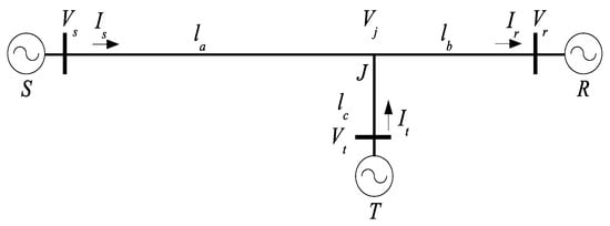
Figure 1. Three-terminal transmission lines.

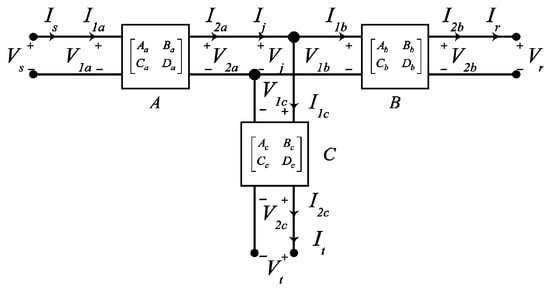
Figure 2. Three-terminal transmission lines for two-port network.

We have

$$\left\{\begin{array}{l}{A}_a=\cosh \left(\gamma l_a\right)=D_a;B_a=Z_c\sinh \left(\gamma l_a\right); C_a=\sinh \left(\gamma l_a\right)/Z_c\\ A_b=\cosh \left(\gamma l_b\right)=D_b;B_b=Z_c\sinh \left(\gamma l_b\right); C_b=\sinh \left(\gamma l_b\right)/Z_c \\ A_c=\cosh \left(\gamma l_c\right)=D_c;B_c=Z_c\sinh \left(\gamma l_c\right); C_c=\sinh \left(\gamma l_c\right)/Z_c\end{array}\right.$$

(1)

where

• $Z_c=x_1+j{x}_2$ is the characteristic impedance of the transmission line;
• $\gamma =x_3+j{x}_4$ is the propagation constant of the transmission line.

2.2. Establishment of Equation EQ1

Using the voltage and current measured at the R-Bus and T-Bus, we establish the relationship equation between the measured voltage at the S-Bus and the calculated voltage.

We determine I_1b from Figure 2 to obtain the following:

$$\left[\begin{array}{l}{V}_{1a}\\ I_{1a}\end{array}\right]=\left[\begin{array}{l}\begin{array}{cc}{A}_a& B_a\end{array}\\ \begin{array}{cc}{C}_a& D_a\end{array}\end{array}\right]\left[\begin{array}{l}{V}_{2a}\\ I_{2a}\end{array}\right]$$

(2)

$$\left[\begin{array}{l}{V}_{1b}\\ I_{1b}\end{array}\right]=\left[\begin{array}{l}\begin{array}{cc}{A}_b& B_b\end{array}\\ \begin{array}{cc}{C}_b& D_b\end{array}\end{array}\right]\left[\begin{array}{l}{V}_{2b}\\ I_{2b}\end{array}\right]$$

(3)

$$\left[\begin{array}{l}{V}_{1c}\\ I_{1c}\end{array}\right]=\left[\begin{array}{l}\begin{array}{cc}{A}_c& B_c\end{array}\\ \begin{array}{cc}{C}_c& D_c\end{array}\end{array}\right]\left[\begin{array}{l}{V}_{2c}\\ I_{2c}\end{array}\right]$$

(4)

We determine I_1b from Figure 2 to obtain the following:

$$I_{1b}=I_j-I_{1c}=I_j-\left(C_c.V_{2c}+D_c.I_{2c}\right)$$

(5)

We determine I_1b from Equation (3), to obtain the following:

$$I_{1b}=C_b.V_{2b}+D_b.I_{2b}$$

(6)

We determine I_j from substituting Equation (5) into Equation (6) to obtain the following:

$$I_j=C_b.V_{2b}+D_b.I_{2b}+C_c.V_{2c}+D_c.I_{2c}$$

(7)

By combining Equation (7) with Equation (3), we obtain the following:

$$\left[\begin{array}{l}{V}_{1b}\\ I_j\end{array}\right]\left[\begin{array}{cccc}\begin{array}{l}{A}_b\\ C_b\end{array}& \begin{array}{l}{B}_b\\ D_b\end{array}& \begin{array}{l}0\\ C_c\end{array}& \begin{array}{l}0\\ D_c\end{array}\end{array}\right]\left[\begin{array}{l}{V}_{2b}\\ I_{2b}\\ V_{2c}\\ I_{2c}\end{array}\right]$$

(8)

According to Figure 2, we have I_j = I_2a and V_1b = V_2a. Substituting into Equation (8) we obtain the following:

$$\left[\begin{array}{l}{V}_{2a}\\ I_{2a}\end{array}\right]\left[\begin{array}{cccc}\begin{array}{l}{A}_b\\ C_b\end{array}& \begin{array}{l}{B}_b\\ D_b\end{array}& \begin{array}{l}0\\ C_c\end{array}& \begin{array}{l}0\\ D_c\end{array}\end{array}\right]\left[\begin{array}{l}{V}_{2b}\\ I_{2b}\\ V_{2c}\\ I_{2c}\end{array}\right]$$

(9)

Substituting Equation (9) into Equation (2) we obtain the following:

$$\left[\begin{array}{l}{V}_{1a}\\ I_{1a}\end{array}\right]\left[\begin{array}{cc}\begin{array}{l}{A}_a\\ C_a\end{array}& \begin{array}{l}{B}_a\\ D_a\end{array}\end{array}\right]\left[\begin{array}{cccc}\begin{array}{l}{A}_b\\ C_b\end{array}& \begin{array}{l}{B}_b\\ D_b\end{array}& \begin{array}{l}0\\ C_c\end{array}& \begin{array}{l}0\\ D_c\end{array}\end{array}\right]\left[\begin{array}{l}{V}_{2b}\\ I_{2b}\\ V_{2c}\\ I_{2c}\end{array}\right]$$

(10)

From Figure 2 we obtain the following:

$$\begin{array}{l}\begin{array}{ccc}{V}_{1a}=V_s;& V_{2b}=V_r;& V_{2c}=V_t\end{array}\\ \begin{array}{ccc}{I}_{1a}=I_s;& I_{2b}=I_r;& I_{2c}=I_t\end{array}\end{array}$$

(11)

Substituting Equation (11) into Equation (10) we obtain the following:

$$\left[\begin{array}{l}{V}_s\\ I_s\end{array}\right]\left[\begin{array}{cc}\begin{array}{l}{A}_a\\ C_a\end{array}& \begin{array}{l}{B}_a\\ D_a\end{array}\end{array}\right]\left[\begin{array}{cccc}\begin{array}{l}{A}_b\\ C_b\end{array}& \begin{array}{l}{B}_b\\ D_b\end{array}& \begin{array}{l}0\\ C_c\end{array}& \begin{array}{l}0\\ D_c\end{array}\end{array}\right]\left[\begin{array}{l}{V}_r\\ I_r\\ V_t\\ I_t\end{array}\right]$$

(12)

According to Equation (12), we can determine the voltage $f_{V_{s1}}$ of the S-Bus and use the voltage and current of the R-Bus and T-Bus.

$$\begin{array}{l}{f}_{V_{s1}}=\left[(A_a{A}_b+B_a{C}_b)V_{r1} +(A_a.B_b+B_a.D_b)I_{r1}\right.\\ \hspace{1em}\hspace{1em}\left.+B_a.C_c.V_{t1}+B_a.D_c.I_{t1}\right]\end{array}$$

(13)

The voltage measured before the S-Bus fault should be equal to the calculated voltage at the S-Bus. We use Equation (13) to obtain the following:

$$\begin{array}{l}EQ1:=V_{s1}-\left[(A_a{A}_b+B_a{C}_b)V_{r1}\right.+(A_a.B_b+B_a.D_b)I_{r1}\\ \left.\hspace{1em}\hspace{1em}\hspace{1em}\hspace{1em}\hspace{1em}\hspace{1em}\hspace{1em}\hspace{1em}\hspace{1em}\hspace{1em}+B_a.C_c.V_{t1}+B_a.D_c.I_{t1}\right]=0\end{array}$$

(14)

where V_s, and I_s, V_r and I_r, and V_t and I_t represent the voltage and current before the fault at the S-Bus, R-Bus, and T-Bus. V_s1 and I_s1 are the voltage and current measured before the S-Bus fault and should be equal to the calculated voltage at the S-Bus. V_r1 and I_r1 are the voltage and current measured before the R-Bus fault and should be equal to the calculated voltage at the R-Bus. V_t1 and I_t1 are the voltage and current measured before the T-Bus fault and should be equal to the calculated voltage at the T-Bus.

2.3. Establishment of Equation EQ2

Using the voltage and current measured at the S-Bus and T-Bus, we establish the following relationship equation between the measured voltage at the R-Bus and the calculated voltage:

$$\left[\begin{array}{l}{V}_{2a}\\ I_{2a}\end{array}\right]=\left[\begin{array}{l}\begin{array}{cc}{A}_a& -B_a\end{array}\\ \begin{array}{cc}-C_a& D_a\end{array}\end{array}\right]\left[\begin{array}{l}{V}_{1a}\\ I_{1a}\end{array}\right]$$

(15)

$$\left[\begin{array}{l}{V}_{2b}\\ I_{2b}\end{array}\right]=\left[\begin{array}{l}\begin{array}{cc}{D}_b& -B_b\end{array}\\ \begin{array}{cc}-C_b& A_b\end{array}\end{array}\right]\left[\begin{array}{l}{V}_{1b}\\ I_{1b}\end{array}\right]$$

(16)

$$\left[\begin{array}{l}{V}_{1c}\\ I_{1c}\end{array}\right]=\left[\begin{array}{l}\begin{array}{cc}{A}_c& B_c\end{array}\\ \begin{array}{cc}{C}_c& D_c\end{array}\end{array}\right]\left[\begin{array}{l}{V}_{2c}\\ I_{2c}\end{array}\right]$$

(17)

We determine the voltage $f_{V_{r1}}$ of the R-Bus and use the voltage and current of the S-Bus and T-Bus. We apply the same analysis as for Equation (13) to obtain the following:

$$\begin{array}{l}{f}_{V_{r1}}=\left[\left(A_c.D_b+B_b.C_c\right)V_t+\left(B_b.D_c+B_c.D_b\right)I_t\right.\\ \hspace{1em}\hspace{1em}+\left.B_b.C_a.V_s-A_a.B_b.I_s\right]\end{array}$$

(18)

The voltage measured before the R-Bus fault should be equal to the calculated voltage at the R-Bus. We use Equation (18) to obtain the following:

$$\begin{array}{l}EQ2:=V_{r1}-\left[\left(A_c.D_b+B_b.C_c\right)V_t\right.+\left(B_b.D_c+B_c.D_b\right)I_t\\ \hspace{1em}\hspace{1em}\hspace{1em}\hspace{1em}\hspace{1em}\hspace{1em}\hspace{1em}\hspace{1em}\hspace{1em}\hspace{1em}\hspace{1em}\left.+ B_b.C_a.V_s-A_a.B_b.I_s\right]=0\end{array}$$

(19)

2.4. Establishment of Equation EQ3

This subfunction assumes that the fault is detected in the SJ segment line. The during-fault positive sequence equivalent circuit for a fault on the SJ segment line is shown in Figure 3. The fault is at distance d_a from the S-Bus. The voltage relationship at fault point F is calculated using the signal from the S-Bus fault, and the voltage at fault point F is calculated using the signal from the J connection point. We use the voltage and current measured from both sides of the fault point to establish a relationship equation for calculating the voltage at the fault point.

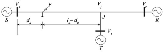
Figure 3. Fault on the SJ segment line.

A fault on the SJ segmented line is shown in Figure 3 as follows:

where d_a is the distance from the starting point S-Bus to the fault point F and where

$$\left\{\begin{array}{l}{A}_{a1}=\cosh \left(\gamma d_a\right)=D_{a1}\\ B_{a1}=Z_c\sinh \left(\gamma d_a\right)\\ C_{a1}=\sinh \left(\gamma d_a\right)/Z_c\\ A_{a2}=\cosh \left(\gamma \left(l_a-d_a\right)\right)=D_{a2}\\ B_{a2}=\sinh \left(\gamma \left(l_a-d_a\right)\right)Z_c\\ C_{a2}=\sinh \left(\gamma \left(l_a-d_a\right)\right)/Z_c\end{array}\right.$$

(20)

We determine V_1b and I_1b from Figure 4 to obtain the following:

$$\left[\begin{array}{l}{V}_{1b}\\ -I_{1b}\end{array}\right]=\left[\begin{array}{l}\begin{array}{cc}{A}_b& B_b\end{array}\\ \begin{array}{cc}{C}_b& D_b\end{array}\end{array}\right]\left[\begin{array}{l}{V}_{2b}\\ -I_{2b}\end{array}\right]$$

(21)

$$\Rightarrow -I_{1b}=C_b.V_{2b}-D_b.I_{2b}$$

(22)

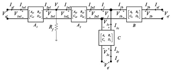
Figure 4. Two-port network with SJ segment line fault.

We determine V_1c and I_1c from Figure 4 to obtain the following:

$$\left[\begin{array}{l}{V}_{1c}\\ -I_{1c}\end{array}\right]=\left[\begin{array}{l}\begin{array}{cc}{A}_c& B_c\end{array}\\ \begin{array}{cc}{C}_c& D_c\end{array}\end{array}\right]\left[\begin{array}{l}{V}_{2c}\\ -I_{2c}\end{array}\right]$$

(23)

$$\Rightarrow -I_{1c}=C_c.V_{2c}-D_c.I_{2c}$$

(24)

We determine I_j from Figure 4 to obtain the following:

$$-I_j=-I_{1b}-I_{1c}$$

(25)

We substitute Equations (22) and (24) into Equation (25) to obtain the following:

$$-I_j=C_b.V_{2b}-D_b.I_{2b}+C_c.V_{2c}-D_c.I_{2c}$$

(26)

By combining Equation (21) with Equation (26), we obtain the following:

$$\left[\begin{array}{l}{V}_{1b}\\ -I_j\end{array}\right]\left[\begin{array}{cccc}\begin{array}{l}{A}_b\\ C_b\end{array}& \begin{array}{l}-B_b\\ -D_b\end{array}& \begin{array}{l}0\\ C_c\end{array}& \begin{array}{l}0\\ -D_c\end{array}\end{array}\right]\left[\begin{array}{l}{V}_{2b}\\ I_{2b}\\ V_{2c}\\ I_{2c}\end{array}\right]$$

(27)

We determine V_1a2 and I_1a2 from Figure 4 to obtain the following:

$$\left[\begin{array}{l}{V}_{1a2}\\ -I_{1a2}\end{array}\right]=\left[\begin{array}{l}\begin{array}{cc}{A}_{a2}& B_{a2}\end{array}\\ \begin{array}{cc}{C}_{a2}& D_{a2}\end{array}\end{array}\right]\left[\begin{array}{l}{V}_{2a2}\\ -I_{2a2}\end{array}\right]$$

(28)

$$\begin{array}{cc}{V}_{2a2}=V_{1b};& -I_{2a2}=-I_j\end{array}$$

(29)

We substitute Equations (27) and (29) into Equation (28) to obtain the following:

$$\left[\begin{array}{l}{V}_{1a2}\\ -I_{1a2}\end{array}\right]\left[\begin{array}{cc}\begin{array}{l}{A}_{a2}\\ C_{a2}\end{array}& \begin{array}{l}{B}_{a2}\\ D_{a2}\end{array}\end{array}\right]\left[\begin{array}{cccc}\begin{array}{l}{A}_b\\ C_b\end{array}& \begin{array}{l}-B_b\\ -D_b\end{array}& \begin{array}{l}0\\ C_c\end{array}& \begin{array}{l}0\\ -D_c\end{array}\end{array}\right]\left[\begin{array}{l}{V}_{2b}\\ I_{2b}\\ V_{2c}\\ I_{2c}\end{array}\right]$$

(30)

From Figure 3 and Figure 4 we obtain the following:

$$\begin{array}{l}\begin{array}{ccc}{V}_{2b}=V_r;& I_{2b}=I_r;& V_{2c}=V_t\end{array};\\ \begin{array}{cc}\begin{array}{c}{V}_{frt}=V_{1a2}\end{array};& I_{frt}=I_{1a2}\end{array}\end{array}$$

(31)

We substitute Equation (31) into Equation (30), which uses the voltage and current measured at the beginning of the R-Bus and T-Bus to determine the voltage V_frt and current I_frt at fault point F, which is shown as follows:

$$\left[\begin{array}{l}{V}_{frt}\\ -I_{frt}\end{array}\right]\left[\begin{array}{cc}\begin{array}{l}{A}_{a2}\\ C_{a2}\end{array}& \begin{array}{l}{B}_{a2}\\ D_{a2}\end{array}\end{array}\right]\left[\begin{array}{cccc}\begin{array}{l}{A}_b\\ C_b\end{array}& \begin{array}{l}-B_b\\ -D_b\end{array}& \begin{array}{l}0\\ C_c\end{array}& \begin{array}{l}0\\ -D_c\end{array}\end{array}\right]\left[\begin{array}{l}{V}_{rf}\\ I_{rf}\\ V_{tf}\\ I_{tf}\end{array}\right]$$

(32)

where V_rf and I_rf and V_tf and I_tf are the voltage and current faults in the R-Bus and T-Bus.

From Figure 4 we obtain the following:

$$\left[\begin{array}{l}{V}_{2a1}\\ I_{2a1}\end{array}\right]=\left[\begin{array}{l}\begin{array}{cc}{D}_{a1}& -B_{a1}\end{array}\\ \begin{array}{cc}-C_{a1}& A_{a1}\end{array}\end{array}\right]\left[\begin{array}{l}{V}_{1a1}\\ I_{1a1}\end{array}\right]$$

(33)

$$\begin{array}{cccc}{V}_{1a1}=V_{sf};& I_{1a1}=I_{sf};& V_{2a1}=V_{fs};& I_{2a1}=I_{fs}\end{array}$$

(34)

We substitute Equation (34) into Equation (33), and use the S-Bus voltage and current to determine the V_fs voltage and I_fs current at fault point F to obtain the following:

$$\left[\begin{array}{l}{V}_{fs}\\ I_{fs}\end{array}\right]=\left[\begin{array}{l}\begin{array}{cc}{D}_{a1}& -B_{a1}\end{array}\\ \begin{array}{cc}-C_{a1}& A_{a1}\end{array}\end{array}\right]\left[\begin{array}{l}{V}_{sf}\\ I_{sf}\end{array}\right]$$

(35)

where V_sf and I_sf are the voltage fault and current fault in the S-Bus.

We determine V_frt from Equation (32) to obtain the following:

$$\begin{array}{l}{V}_{frt}=(A_{a2}.A_b+B_{a2}.C_b)V_{rf}-(A_{a2}.B_b-B_{a2}.D_b)I_{rf}\\ \hspace{1em}\hspace{1em}\hspace{1em}\hspace{1em}\hspace{1em}\hspace{1em}\hspace{1em}\hspace{1em}\hspace{1em}\hspace{1em}\hspace{1em}\hspace{1em}+B_{a2}.C_c.V_{tf}-B_{a2}.D_c.I_{tf}\end{array}$$

(36)

We determine V_fs from Equation (35) to obtain the following:

$$V_{fs}=D_{a1}.V_{sf}-B_{a1}.I_{sf}$$

(37)

We substitute Equation (36) into Equation (37) to obtain the following:

$$\begin{array}{l}EQ3:=\left(D_{a1}.V_{sf}-B_{a1}.I_{sf}\right) -\left[(A_{a2}.A_b+B_{a2}.C_b)V_{rf}\right.\\ \hspace{1em}\hspace{1em}\hspace{1em}-(A_{a2}.B_b-B_{a2}.D_b)I_{rf}\left.+B_{a2}.C_c.V_{tf}-B_{a2}.D_c.I_{tf}\right]=0\end{array}$$

(38)

2.5. Establishment of Equations EQ4

This subfunction assumes that the fault is on an RJ segment line. The during-fault positive sequence equivalent circuit for a fault on an RJ segmented lines is shown in Figure 5. The fault is at distance d_b from the R-Bus. The voltage relationship at fault point F is calculated using the signal from the R-Bus fault, and the voltage at fault point F is calculated using the signal from the J connection point. We use the voltage and current measured from both sides of the fault point to establish a relationship equation for calculating the voltage at the fault point.

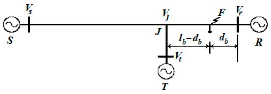
Figure 5. Fault on the RJ segment line.

For a fault on the RJ segment line, see Figure 5 and Figure 6 as follows:

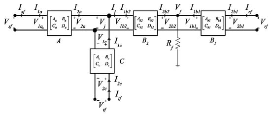
Figure 6. Two-port network with RJ segment line fault.

where

$$\left\{\begin{array}{l}{A}_{b1}=\cosh \left(\gamma d_b\right)=D_{b1}\\ B_{b1}=Z_c\sinh \left(\gamma d_b\right)\\ C_{b1}=\sinh \left(\gamma d_b\right)/Z_c\\ A_{b2}=\cosh \left(\gamma \left(l_b-d_b\right)\right)=D_{b2}\\ B_{b2}=\sinh \left(\gamma \left(l_b-d_b\right)\right)Z_c\\ C_{b2}=\sinh \left(\gamma \left(l_b-d_b\right)\right)/Z_c\end{array}\right.$$

(39)

We apply the same analysis as for Equation (38) to obtain the following:

$$\begin{array}{l}EQ4:=\left(A_{b1}.V_{rf}-B_{b1}.I_{rf}\right) -\left[\left(A_c.D_{b2}+B_{b2}.C_c\right)V_{tf}\right.\\ \hspace{1em}\hspace{1em}\hspace{1em}\hspace{1em}-\left(B_{b2}.D_c+B_c.D_{b2}\right)I_{tf}\\ \left.\begin{array}{ccc}& & \end{array}\hspace{1em}\hspace{1em}+B_{b2.}{C}_a.V_{sf}-A_a.B_{b2}.I_{sf}\right]=0\end{array}$$

(40)

where V_sf and I_sf are the voltage fault and current fault in the S-Bus.

2.6. Establishment of Equations EQ5

This subfunction assumes that the fault is with a TJ segment line. The during-fault positive sequence equivalent circuit for a fault on a TJ segment line is shown in Figure 7. The fault is at distance d_c from the T-Bus. The voltage relationship at fault point F is calculated using the signal from the T-Bus fault, and the voltage at fault point F is calculated using the signal from the J connection point. We use the voltage and current measured from both sides of the fault point to establish a relationship equation for calculating the voltage at the fault point.

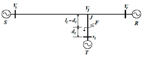
Figure 7. Fault on the TJ segment line.

For a fault on the TJ segmented lines, see Figure 7 and Figure 8 as follows:

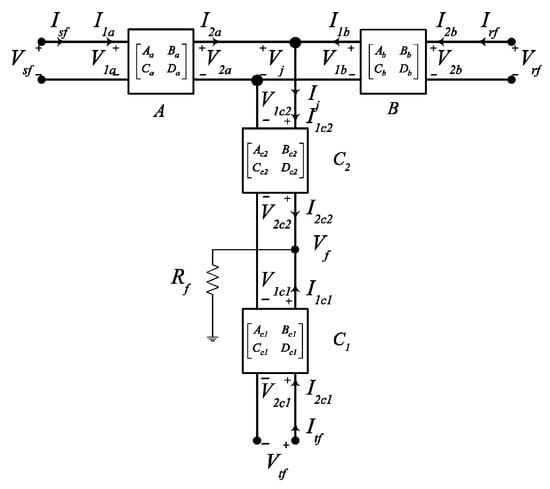
Figure 8. Two-port network with TJ segment line fault.

where

$$\left\{\begin{array}{l}{A}_{c1}=\cosh \left(\gamma d_c\right)=D_{c1}\\ B_{c1}=Z_c\sinh \left(\gamma d_c\right)\\ C_{c1}=\sinh \left(\gamma d_c\right)/Z_c\\ A_{c2}=\cosh \left(\gamma \left(l_c-d_c\right)\right)=D_{c2}\\ B_{c2}=Z_c\sinh \left(\gamma \left(l_c-d_c\right)\right)\\ C_{c2}=\sinh \left(\gamma \left(l_c-d_c\right)\right)/Z_c\end{array}\right.$$

(41)

We apply the same analysis as for Equation (38) to obtain the following:

$$\begin{array}{l}EQ5:=\left(A_{c1}.V_{tf}-B_{c1}.I_{tf}\right) -\left[\left(B_{c2}.C_a+D_a.D_{c2}\right)V_{sf}\right.\\ -\left(A_a.B_{c2}+B_a.D_{c2}\right)I_{sf}\\ \left.\begin{array}{ccc}& & \end{array} +B_{c2}.C_b.V_{rf}-B_{c2}.D_b.I_{rf}\right]=0\end{array}$$

(42)

2.7. Fault Distance Measurement and Positioning Algorithm

EQ1, EQ2, and EQ3 comprise three complex equations. To solve complex equation systems, we decompose the positive sequence component value and negative sequence value parts into a system of equations, as shown below.

Fault location distance measurement in SJ segment line is as follows:

$$\left\{\begin{array}{l}{f}_1\left(x_1,x_2,x_3,x_4,x_5\right)=real\left(EQ1\right)=0\\ f_2\left(x_1,x_2,x_3,x_4,x_5\right)=imag\left(EQ1\right)=0\\ f_3\left(x_1,x_2,x_3,x_4,x_5\right)=real\left(EQ2\right)=0\\ f_4\left(x_1,x_2,x_3,x_4,x_5\right)=imag\left(EQ2\right)=0\\ f_{5SJ}\left(x_1,x_2,x_3,x_4,x_5\right)=real\left(EQ3\right)=0\end{array}\right.$$

(43)

Fault location distance measurement in RJ segment line is as follows:

$$\left\{\begin{array}{l}{f}_1\left(x_1,x_2,x_3,x_4,x_5\right)=real\left(EQ1\right)=0\\ f_2\left(x_1,x_2,x_3,x_4,x_5\right)=imag\left(EQ1\right)=0\\ f_3\left(x_1,x_2,x_3,x_4,x_5\right)=real\left(EQ2\right)=0\\ f_4\left(x_1,x_2,x_3,x_4,x_5\right)=imag\left(EQ2\right)=0\\ f_{5RJ}\left(x_1,x_2,x_3,x_4,x_5\right)=real\left(EQ4\right)=0\end{array}\right.$$

(44)

Fault location distance measurement in TJ segment line is as follows:

$$\left\{\begin{array}{l}{f}_1\left(x_1,x_2,x_3,x_4,x_5\right)=real\left(EQ1\right)=0\\ f_2\left(x_1,x_2,x_3,x_4,x_5\right)=imag\left(EQ1\right)=0\\ f_3\left(x_1,x_2,x_3,x_4,x_5\right)=real\left(EQ2\right)=0\\ f_4\left(x_1,x_2,x_3,x_4,x_5\right)=imag\left(EQ2\right)=0\\ f_{5TJ}\left(x_1,x_2,x_3,x_4,x_5\right)=real\left(EQ5\right)=0\end{array}\right.$$

(45)

Equations (43)–(45) are nonlinear equations with five positive sequence component. We use the fsolve function in MATLAB software to solve a system of nonlinear equations arising from the optimization problem and search numerical methods in the trust domain, selecting 1 × 10⁻⁵ as the initial solution value for five positive sequence components.

We apply the following conditions to determine the location of the fault:

$$\begin{array}{l}\left\{\begin{array}{l}fval\left(f_{5SJ}\right)\le fval\left(f_{5RJ}\right)\\ fval\left(f_{5SJ}\right)\le fval\left(f_{5TJ}\right)\end{array}\right.\to d=d_a\\ \left\{\begin{array}{l}fval\left(f_{5RJ}\right)\le fval\left(f_{5TJ}\right)\\ fval\left(f_{5RJ}\right)\le fval\left(f_{5SJ}\right)\end{array}\right.\to d=d_b\\ \left\{\begin{array}{l}fval\left(f_{5TJ}\right)\le fval\left(f_{5SJ}\right)\\ fval\left(f_{5TJ}\right)\le fval\left(f_{5RJ}\right)\end{array}\right.\to d=d_c\end{array}$$

(46)

where fval (f_5SJ), fval (f_5RJ), and fval (f_5TJ) are the values of f_5SJ, f_5RJ, and f_5TJ, replacing the values of $x_1,x_2,x_3,x_4,x_5$, and d_a, d_b, and d_c, respectively. d_a, d_b, and d_c is the distance from the starting point on the S-Bus, R-Bus, and T-Bus to the fault point F. The digital data records of all terminals in the activation circuit are used to record synchronous measurements before and after the fault. We calculate the values of $x_1,x_2,x_3,x_4$, and $x_5$. The characteristic impedance of the transmission lines is given by $Z_c=x_1+j{x}_2$. The propagation constant of the transmission lines is given by $\gamma =x_3+j{x}_4$. The distance from the starting-point terminal to the fault point F is given by $d=x_5$. If the fault is on the SJ segment line then we have d = d_a. If the fault is on the RJ segment line then we have d = d_b. If the fault is on the TJ segment line then we have d = d_c.

The algorithm for determining the above line parameters and fault location is summarized as an algorithm diagram, as shown in Figure 9:

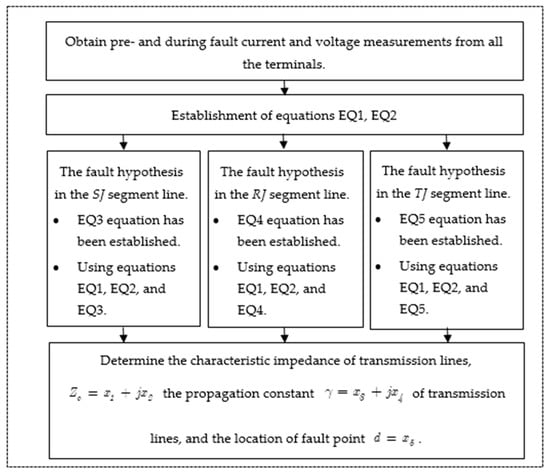
Figure 9. Suggested solution structure, including input signal, steps involved, and output parameters.

3. Experimental Results

3.1. Simulation Fault Location Methods on Transmission Lines Do Not Use Lines Parameters and Experimental Testing

In order to verify the effectiveness and correctness of our algorithm, this paper used the parameters of 220 kV, 50 Hz high-voltage transmission lines in MATLAB/Simulink simulation software. Numerical simulation was conducted based on a three-terminal transmission lines system [18]. The lengths of the segments were l_a = 200 km, l_b = 100 km, and l_c = 150 km. The line parameters for the positive sequence R₁ = 0.02083 (Ω/km), L₁ = 0.89848 (mH/km), and C₁ = 0.0129 (μF/km); while for the zero sequence, they are R₀ = 0.1148 (Ω/km), L₀ = 2.2886 (mH/km), and C₀ = 0.00523 (μF/km). The initial phase of the three-terminal power supply of the system is arg $E_s\angle 0°$, arg $E_R\angle 20°$, and arg $E_T\angle 40°$.

3.1.1. Simulation Fault Location Methods

Fault characteristics are predominantly determined by fault location and fault resistance in Figure 10. To evaluate the impact of fault severity on the proposed method, a phase-to-phase (AB) short-circuit fault was simulated on the SJ segment line at 50 km from the S-bus with 50 Ω fault resistance. The simulation results are as follows: $x_1=0.0048$, $x_2=-0.0002$, $x_3=0.0001$, $x_4=0.0011$, and $x_5=49.9995$. The characteristic impedance of transmission lines is given by $Z_c=0.0048-j0.0002$. The propagation constant of transmission lines is given by $\gamma =0.0001+j0.0011$. The distance from the starting-point terminal to the fault point F is given by $d_a=49.9995$.

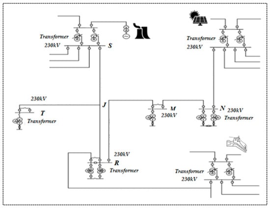
Figure 10. System configuration comprises a three-terminal transmission line.

The fault resistances were 50 Ω, 100 Ω, 150 Ω, and 200 Ω. The results indicate that the proposed algorithm is effective for different fault distances, and that different transition resistances are effective. Therefore, our protection algorithm does not require the use of line selection algorithms nor the influence of output circuit parameters.

For line fault on the SJ segment line the accuracy of fault location, measured as a percentage error, is presented in Table 1.

Table 1. Simulation results demonstrate the effects of different faults, such as fault location and fault resistance, on the SJ segment line.

Fault Type	Fault Resistance in Ω	Fault Location in km						Percentage Error ei%
		50	75	100	125	150	175
AG	50	49.993	75.011	100.016	125.018	150.001	174.980	−0.010
	100	49.996	75.019	100.025	125.029	149.999	174.962	−0.019
	150	49.998	75.027	100.034	125.041	149.997	174.945	−0.028
	200	49.999	75.035	100.044	125.053	149.996	174.928	−0.036
AB	50	49.999	75.005	100.007	125.009	150.003	174.995	0.004
	100	49.998	75.008	100.010	125.012	150.001	174.988	−0.006
	150	49.999	75.010	100.013	125.016	150.000	174.981	−0.010
	200	50.000	75.013	100.016	125.020	149.999	174.975	−0.013
ABG	50	49.993	75.005	100.007	125.009	150.003	174.997	0.004
	100	49.995	75.007	100.009	125.011	150.001	174.990	0.005
	150	49.997	75.009	100.012	125.014	150.000	174.984	−0.008
	200	49.999	75.012	100.015	125.018	149.999	174.978	−0.011
ABC	50	49.999	75.003	100.004	125.006	150.003	175.002	0.003
	100	49.999	75.005	100.006	125.007	150.002	174.997	0.003
	150	49.999	75.006	100.007	125.009	150.001	174.994	0.004
	200	49.999	75.007	100.009	125.011	150.001	174.990	0.005

Fault location % Error is as follows:

$$\%Error={\displaystyle \frac{Actual length-Estimated location}{Total length of line}}\times 100$$

(47)

Table 1 shows the locations of faults that occurred on a three-terminal transmission line. Our algorithm does not require line parameters and only uses the positive components of on-site measurement signals, so it can be applied to the localization of all types of problems without the need for classification algorithms. Using MATLAB software the effectiveness and accuracy of the proposed algorithm were simulated and tested. Table 1 presents the fault location algorithm’s performance across various fault types. For single-phase-to-ground (AG) short-circuit faults with different fault resistances, the algorithm achieved a 0.036% location error. The corresponding errors were 0.013% for phase-to-phase (AB) faults, 0.011% for two-phase-to-ground (ABG) faults, and 0.005% for three-phase (ABC) faults.

The simulation results show that the proposed algorithm provides positive results, with a positioning error of no more than 0.036% for typical types of fault AG, AB, ABG, and ABC, and a segment length of l = 200 km, indicating the accuracy of the algorithm.

Table 2 shows line faults on the TJ and RJ segment line. The accuracy of fault location, measured as percentage error, is presented. The accuracy of fault location, measured as a percentage error, is high. For single-phase-to-ground (AG) short-circuit faults in the TJ segment line with varying fault resistances, the algorithm achieves a location error of 0.027%. Similarly, for faults in the RJ segmented line, it achieves an error of 0.028%. For phase-to-phase (AB) short-circuit faults in the TJ segment line with varying fault resistances, the algorithm achieves a location error of 0.038%. Similarly, for faults in the RJ segmented line, it achieves an error of 0.034%.

Table 2. Simulation results demonstrate the effects of different faults, such as fault location and fault resistance, on the TJ and RJ segment line.

Fault Section	Fault Type	Fault Resistance in Ω	Fault Location in km						Percentage Error ei%
			35	45	55	65	75	85
TJ	AG	50	35.000	45.012	55.006	65.015	74.970	84.982	0.020
		100	35.002	45.017	54.960	64.985	74.988	84.989	−0.027
		150	35.013	44.976	54.985	64.988	74.988	84.988	0.016
		200	34.971	44.985	54.986	64.987	74.986	84.986	−0.019
RJ	AG	50	35.014	45.030	55.011	64.987	74.982	84.983	0.030
		100	35.031	45.011	54.987	64.962	74.986	84.988	−0.038
		150	35.019	44.995	54.967	64.965	74.987	84.988	−0.035
		200	35.009	44.982	54.950	64.967	74.987	84.987	−0.033
TJ	AB	50	35.000	45.000	55.001	65.003	74.958	84.986	−0.028
		100	35.000	45.001	55.012	64.972	74.993	84.994	−0.018
		150	35.000	45.013	54.983	64.991	74.993	84.993	−0.012
		200	35.004	44.977	54.990	64.991	74.992	84.992	−0.016
RJ	AB	50	35.015	45.034	55.019	65.007	74.983	84.970	0.034
		100	35.038	45.032	55.003	64.995	74.968	84.967	0.032
		150	35.030	45.030	54.985	64.984	74.966	84.974	0.030
		200	35.023	45.031	54.967	64.975	74.985	84.969	0.031

3.1.2. Effect of Noise

In this test, one percent (1%) of the peak-to-peak value of the input signals was set as noise and was added to the three terminals of Figure 3. Figure 11 exhibits the pre-fault three-phase voltage waveform with 1% noise on the S-Bus. From the results in Table 3, it can be seen that in all cases the fault localization error is 0.027%.

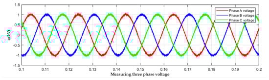
Figure 11. Pre-fault three-phase voltage signals with 1% noise.

Table 3. Fault location results considering 1% signal noise.

Fault Type	Fault Resistance in Ω	Fault Location in km						Percentage Error ei%
		50	75	100	125	150	175
AG	50	49.998	74.999	100.003	124.997	149.977	174.986	0.012
	100	49.994	74.995	99.999	124.992	149.973	174.974	0.013
	150	49.990	74.991	99.996	124.988	149.967	174.960	0.020
	200	49.987	74.987	99.994	124.983	149.961	174.946	0.027
AB	50	49.997	74.998	100.000	125.003	149.995	174.996	0.003
	100	49.994	74.995	99.999	124.998	149.989	174.988	0.006
	150	49.992	74.993	99.998	124.995	149.984	174.979	0.010
	200	49.990	74.991	99.997	124.992	149.979	174.970	0.015

When simulating all the listed scenarios with the incorporation of 1% noise, it becomes apparent that the resultant positioning errors, albeit present, do not significantly alter the overall outcome in any of the cases.

In scenarios involving the localization of wireless signals or the positioning of sensors within a network, the inclusion of 1% noise resulted in slight shifts in the calculated positions. However, those shifts were insufficient to alter the overall layout or the relationships between the various nodes. Across all scenarios, the positioning errors remained within acceptable margins, ensuring that the incorrect localization did not sway the final assessment nor the conclusions drawn from the simulations. This demonstrates the robustness of the simulation methods and their ability to provide reliable results even in the presence of noise.

3.1.3. Effect of One Outage/Maintenance Line Branch

Sometimes, for maintenance or planning purposes, one of the three terminal lines are disconnected, commonly referred to as a nonservice line branch [19]. Consider the same circuit shown in Figure 3, but now the T-Bus circuit breaker (CB) has been disconnected. In other words, there is no power supply through the TJ segment line.

The occurrence of one of the three terminal lines being disconnected in electrical systems, particularly when a single station loses power but continues generating electricity, necessitates an evaluation of its impact on simulation-based location methods. To this end, we conducted a series of rigorous studies and experiments to ascertain the effects. From the results in Table 4, it can be seen that in all cases the fault localization error is 0.025%. In our simulated environment we specifically designed a scenario where one station lost power. By comparing the simulation results before and after the outage, we found that the accuracy of the location method did not exhibit any notable decline.

Table 4. Influence of the effect of one outage on the location method simulation.

Fault Type	Fault Resistance in Ω	Fault Location in km						Percentage Error ei%
		50	75	100	125	150	175
AG	50	50.001	75.002	99.997	124.996	149.992	174.988	0.012
	100	50.014	75.003	99.994	124.989	149.975	174.966	0.017
	150	49.977	74.982	99.976	124.972	149.986	174.951	0.024
	200	49.988	74.970	100.010	125.048	150.006	175.017	0.024
AB	50	50.018	75.009	100.010	124.994	149.989	174.984	0.009
	100	49.975	74.987	100.001	124.959	149.977	174.987	0.020
	150	49.983	74.970	100.000	125.017	150.018	175.021	0.015
	200	49.950	74.978	100.000	125.001	150.035	175.044	0.025

3.1.4. Influence of Current Transformer (CT) Saturation

When a short-circuit fault occurs in a power system, the amplitude of the alternating current (AC) and the direct current component (DC) in the short-circuit current makes the current transformer become saturated. Consequently, the output current waveform of the current transformer is distorted, causing the malfunction of the protective relay system because the amplitude of the secondary current in cases of current transformer saturation is smaller than that of the actual short-circuit current. Consider a severe current transformer saturation situation. The degree of saturation is defined according to [20], as follows, to quantify the level of saturation:

$$Degree of Saturation=1-{\displaystyle \frac{I_{2sat}}{I_{2ideal}}}$$

(48)

where I_2sat and I_2ideal are, respectively, the one-cycle root mean square of the secondary-side saturated current and the ideal current, including DC offset. The cycle is evaluated only after saturation has started. Thereby, Equation (47) is a value between 0 and 1, where 0 represents no saturation and 1 represents no output from CT throughout the entire cycle. The saturation current of the second party is measured from the CT on the S-Bus, and the saturation degree of phases A, B, and C can be calculated using Equation (47). Therefore, the three-phase saturation current is severely distorted by the CT saturation phenomenon, where the saturation degree represents the saturation as heavy [20].

The secondary-side saturation fault currents measured from the CT on the S-Bus of Figure 3 are plotted in Figure 12 with a fault resistance 0.1 Ω. The acquired fault location was determined to be 5 km away from the S-Bus. The error in the fault location was found to be 0.025%. From the results of the proposed method, it is evident that it is not affected by the severe waveform distortion caused by CT saturation. Therefore, the analysis of the results clearly indicates that the proposed method remains relatively unaffected by severe waveform distortion resulting from CT saturation. In scenarios where CT saturation does occur, the steady-state component of the voltage signal continues to provide a reliable basis for measurement and analysis. Furthermore, the introduction of CT saturation compensation techniques holds the potential to significantly reduce or even eliminate the errors associated with CT saturation. Such techniques are outlined in [21].

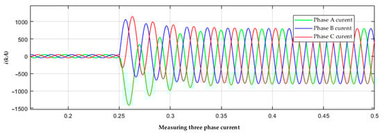
Figure 12. Secondary-side three-phase saturation fault currents measured from S-Bus.

3.2. Comparison with the Technique

Table 5 lists the ranging results of both the fault analysis-based method proposed in this paper and the method proposed in reference [18]. According to Table 5, both methods can accurately determine the fault branch and calculate the accurate fault distance in the case of a grounded fault. And this article proposes a method for fault location to obtain high-precision ranging results.

Table 5. Comparison of different fault parameters, including fault location and fault resistance.

Fault Type	Fault Resistance in Ω	Fault Location in km	Proposed Method		Reference [18] Method
			Location	Error %	Location	Error %
AG	50	50	49.993	0.003	49.865	0.067
		100	100.016	−0.008	99.905	0.047
		150	150.001	−0.001	149.945	0.028
	100	50	49.996	0.002	49.845	0.078
		100	100.025	−0.013	99.875	0.063
		150	149.999	0.001	149.905	0.047
	150	50	49.998	0.001	49.805	0.098
		100	100.034	−0.017	99.865	0.068
		150	149.997	0.001	149.915	0.043
ABG	50	50	49.993	0.003	50.075	−0.038
		100	100.007	−0.004	100.115	−0.057
		150	150.003	−0.001	150.075	−0.037
	100	50	49.999	0.000	49.123	0.439
		100	100.009	−0.005	99.865	0.068
		150	150.001	−0.001	149.905	0.047
	150	50	49.999	0.000	49.785	0.108
		100	100.012	−0.006	99.895	0.053
		150	150.000	0.000	149.945	0.028

The above simulation results were obtained under ideal conditions, assuming complete synchronization of the three-terminal data and ignoring the influence of measurement errors. As shown in Table 5, the comparative results demonstrate that for single-phase-to-ground (AG) faults on the SJ segment line with varying fault resistances, the proposed algorithm achieves a location error of 0.017%, significantly outperforming the method in [18] (0.078%). Similarly, for phase-to-phase (AB) faults, our method yields an error of just 0.006% compared to 0.068% from the reference approach. The method proposed for fault localization demonstrates superior performance compared to the fault localization reference method. It also demonstrates higher adaptability and flexibility for different fault parameters, including fault location and fault resistance. In contrast, although the method in [18] may be effective in certain specific situations, it will shorten the overall efficiency and accuracy.

4. Discussion

Nowadays, fault location techniques can mainly be divided into the following three categories: impedance-based approaches, traveling wave methods, and artificial intelligence methods. In impedance-based approaches, the algorithm is not complicated; however, the positioning results are affected by the value of the fault resistance and the load current, and by the input data of the algorithm requiring prior knowledge of the line parameters [5]. The traveling wave method is not affected by the structure lines but is reliant on the accurate extraction of transient traveling waves, the identification and calibration of reflected waves at the fault point, the determination of wave velocity, and the need to improve the ranging accuracy of the fault location device. This method uses transient faults on waveforms such as traveling waves to locate faults and is slightly affected by load variance and high fault resistance [9]. In turn, artificial intelligence methods can be applied to larger size problems in accordance with different design and training procedures. With the support of industrial digitalization, the transmission network has accumulated a large number of data samples by using machine learning. However, the methods are still complicated due to their wide scope of data collection, model training, and time consumption [12]. Power system requirements continue to evolve. Unlike conventional methods that rely on line parameters, the proposed fault location algorithm removes these dependencies, enhancing reliability. However, the location results have certain errors [15]. Our algorithm uses the positive sequence component values of voltage and current which are synchronously measured from the end of the transmission line. The digital data records of all terminals in the activation circuit will be used to record synchronous measurements before and after the fault, and do not require the use of a fault classification algorithm nor transmission line parameters. The method estimates the characteristic impedance and propagation constants of the transmission lines and pinpoints the fault location.

5. Conclusions

Due to the fact that errors in the calculation process of transmission lines parameters must go through a series of intermediate calculations, it is impossible to accurately determine transmission lines parameters. If the transmission lines parameter measurement method is used, the fault location results will still have errors due to measurement errors. Our algorithm determines the faults that occur on forked transmission lines and segments with the same wire type. The new feature of this algorithm is that the input of the algorithm does not require line parameters, so when the transmission line parameters are incorrect the positioning results will not be affected. Our algorithm uses the sequential components of the measurement signal, so it can locate various types of events without the need for event classification algorithms. The fault location results demonstrate the accuracy and effectiveness of the algorithm.

Our algorithm can be applied for fault localization occurring on a multi-terminal transmission line. It uses the positive sequence component values of voltage and current synchronously measured from the end of the line before and during the fault to determine the sum of source impedances. Combined with the total impedance of the transmission lines, a total impedance matrix of the power grid can be established, and iterative algorithms can be applied to locate the problem. This algorithm can be applied to the fault localization of various faults, and the localization results are not affected by short-circuit resistance. The simulation results demonstrate that the proposed algorithm effectively determines impedance, transfer constant, and fault location with a positioning error of no more than 0.038%. The proposed fault localization method outperforms the reference method [20], offering greater adaptability and flexibility across different fault parameters like location and resistance. It can be discerned from the simulations that the proposed method is only slightly affected by CT saturation and signals with noise. It can further demonstrate the accuracy of the proposed method.

References

- Izykowski, J. “Fault Location on Power Transmission Lines”, Wroclaw. 2008. Available online: https://www.dbc.wroc.pl/dlibra/publication/2583/edition/2599/content (accessed on 7 January 2021).
- Badran, O.; Rizk, M.E.; Abulanwar, S. Comprehensive fault reporting for three-terminal transmission line using adaptive estimation of line parameters. Electr. Power Syst. Res. 2023, 223, 109536. [Google Scholar] [CrossRef]
- Poudineh-Ebrahimi, F.; Ghazizadeh-Ahsaee, M. Accurate fault location algorithm for three-terminal lines without time synchronization considering unknown and different parameters of sections. Electr. Power Syst. Res. 2022, 211, 108057. [Google Scholar] [CrossRef]
- Chafi, Z.S.; Afrakhte, H. Wide area fault location on transmission systems using synchronized/unsynchronized voltage/current measurements. Electr. Power Syst. Res. 2021, 197, 107285. [Google Scholar] [CrossRef]
- Li, C.X.; Liu, G.W.; Yu, C.; Wang, C.; Chen, F.B.; Wan, S.M. A fault location method for high-voltage transmission lines based on traveling wave. J. Electr. Power Sci. Technol. 2023, 38, 80–84. [Google Scholar] [CrossRef]
- Atuchukwu, J.A.; Obinna, O.K.; Ugochukwu, A.E. Location of Fault on Transmission Line using Traveling Wave Technique. Eur. J. Energy Res. 2022, 2736–5506. [Google Scholar] [CrossRef]
- Ding, J.L.; Wang, X.; Zheng, Y.H.; Li, L. Distributed Traveling-Wave-Based Fault-Location Algorithm Embedded in Multiterminal Transmission Lines. IEEE Trans. Power Deliv. 2018, 33, 3045–3054. [Google Scholar] [CrossRef]
- Huang, Y.; Zhang, G.B.; Wang, Q.; Shu, H.C. Faulted traveling waves for transmission lines based on image features. Trans. China Electro Tech. Soc. 2023, 38, 1340–1352. [Google Scholar] [CrossRef]
- Deng, F.; Mei, L.J.; Tang, X.; Xu, F.; Zeng, X.J. Faulty line selection method of distribution network based on time-frequency traveling wave panoramic waveform. Trans. China Electro Tech. Soc. 2021, 36, 2861–2870. [Google Scholar] [CrossRef]
- He, J.H.; Luo, G.M.; Cheng, M.X.; Liu, Y.M.; Tan, Y.J.; Li, M. A research review on application of artificial intelligence in power system fault analysis and location. Proc. CSEE 2020, 40, 5506–5515. [Google Scholar] [CrossRef]
- Zhou, N.C.; Xiao, S.Y.; Yu, Y.S.; Wang, G.Q. Fault location in distribution networks based on centroid frequency and BP neural networks. Trans. China Electro Tech. Soc. 2019, 33, 4155–4166. [Google Scholar] [CrossRef]
- Soham, C.; Satarupa, C.; Aleena, S. A review on various artificial intelligence techniques used for transmission line fault location. In Proceedings of the 2018 3rd International Conference on Inventive Computation Technologies (ICICT), Coimbatore, India, 15–16 November 2018; IEEE Xplore Part Number: CFP18F70-ART. pp. 105–109, ISBN 978-1-5386-4985-5. [Google Scholar]
- Junsoo, C.; Jaedeok, P.; Gihun, P.; Taesik, P. A new fault location identification method for transmission line using machine learning algorithm. In Proceedings of the 2019 3rd International Conference on Smart Grid and Smart Cities (ICSGSC), Berkeley, CA, USA, 25–28 June 2019; pp. 81–84. [Google Scholar] [CrossRef]
- Özdemir, Ö.; Köker, R.; Pamuk, N. Fault Classification and Precise Fault Location Detection in 400 kV High-Voltage Power Transmission Lines Using Machine Learning Algorithms. Processes 2025, 13, 527. [Google Scholar] [CrossRef]
- Abasi, M.; Rohani, A.; Hatami, F.; Joorabian, M.; Gharehpetian, G.B. Fault location determination in three-terminal transmission lines connected to industrial microgrids without requiring fault classification data and independent of line parameters. Int. J. Electr. Power Energy Syst. 2021, 131, 107044. [Google Scholar] [CrossRef]
- Davoudi, M.; Sadeh, J.; Kamyab, E. Transient-Based Fault Location on Three-Terminal and Tapped Transmission Lines Not Requiring Line Parameters. IEEE Trans. Power Deliv. 2018, 33, 179–188. [Google Scholar] [CrossRef]
- Alexander, C.K.; Sadiku, M.N.O. Fundamentals of Electric Circuits; McGraw-Hill: New York, NY, USA, 2009; p. 792. [Google Scholar]
- Zhu, Z.F.; Chen, X.F.; Zhang, Y.C.; Guo, C.; Qiao, D. A new fault location algorithm for T-type Transmission lines based on phase recognition. Conf. Ser. Mater. Sci. Eng. 2018, 339, 012012. [Google Scholar] [CrossRef]
- Lee, Y.J.; Chao, C.H.; Lin, T.C.; Liu, C.W. A Synchrophasor-Based Fault Location Method for Three-Terminal Hybrid Transmission Lines With One Off-Service Line Branch. IEEE Trans. Power Deliv. 2018, 33, 3249–3251. [Google Scholar] [CrossRef]
- Stanbury, M.; Djekic, Z. The Impact of Current-Transformer Saturation on Transformer Differential Protection. IEEE Trans. Power Deliv. 2015, 30, 1278–1287. [Google Scholar] [CrossRef]
- Kang, Y.C.; Lim, U.J.; Kang, S.H. Compensating algorithm suitable for use with measurement-type current transformers for protection. IEEE Proc. Gener. Transm. Distrib. 2006, 152, 880–890. [Google Scholar] [CrossRef]
Disclaimer/Publisher’s Note: The statements, opinions and data contained in all publications are solely those of the individual author(s) and contributor(s) and not of MDPI and/or the editor(s). MDPI and/or the editor(s) disclaim responsibility for any injury to people or property resulting from any ideas, methods, instructions or products referred to in the content. |
© 2025 by the authors. Licensee MDPI, Basel, Switzerland. This article is an open access article distributed under the terms and conditions of the Creative Commons Attribution (CC BY) license (https://creativecommons.org/licenses/by/4.0/).