Abstract
In the context of the Jammertest 2023, a collaborative experiment was carried out by the European Commission Joint Research Centre (JRC), the European Space Operations Centre of ESA (ESOC), the Norwegian Communication Authority, and the Norwegian Defense Research Establishment (FFI) to explore potential RF interference monitoring in the navigation GNSS band from LEO. The experiment utilizes the ESA OPS-SAT satellite and the possibility of transmitting a custom jamming signal pattern during the Jammertest event. The objective is to validate the feasibility of detecting and locating ground-generated jamming signals using SDR technology on-board LEO. The insight into the signal structure and location provides a unique chance to assess the performance and limitations of this approach in a real-world scenario. This paper presents the processing of raw RF data collected during the in-flight experiment, including the generation of frequency difference of arrival (FDOA) observables and emitter geolocation. Despite the constraints posed by onboard resources and mission limitations, this work offers a persuasive proof of concept and suggests new guidelines for implementing this technology on future LEO missions.
1. Introduction
The significance of Global Navigation Satellite Systems (GNSS) in providing accurate positioning, navigation, and timing services for various applications cannot be overstated. However, these essential systems are vulnerable to interference from natural and man-made sources, which could lead to potential disruptions and inaccuracies in the received signals. As a result, there has been a growing focus on developing efficient Radio Frequency Interference (RFI) monitoring techniques, with a particular emphasis on space-based solutions. The use of Low Earth Orbit (LEO) satellites has emerged as an attractive tool for detecting and locating terrestrial RFI, providing improved wide-area coverage and the potential to be less affected by ground disturbances.
Nevertheless, concerns persist regarding the effectiveness and reliability of these in-space detection methods, particularly in terms of the complexity, cost, and onboard resources needed to address this challenge. The approach necessitates further research covering various, such as the exploitation of single [1,2] and multiple satellites working in tandem [3], new detection and localization techniques, and the availability of New Space hardware and software technologies.
The OPS-SAT experiment aligns with this objective and provides an unprecedented in-flight demonstration of LEO-based RFI monitoring, even with nanosatellite low-cost technology and strict onboard resource constraints. In September 2023, the European Commission’s Joint Research Centre (JRC), in collaboration with the European Space Operations Centre of ESA (ESOC), the Norwegian Communication Authority, and the Norwegian Defense Research Establishment (FFI), envisioned exploiting ESA’s OPS-SAT LEO satellite and its onboard SDR (Software Defined Radio) [4] to conduct an experiment aimed at monitoring GNSS interference emissions generated on the ground. The concept originated from the unique opportunity presented by FFI to conduct experimentation during the Jammertest 2023 event [5]. This framework provides a one-of-a-kind chance to perform RFI tests in a controlled environment, replicating the necessary conditions to stimulate and validate RFI detection and localization from the OPS-SAT LEO satellite as it passes over the Norwegian Andøya site.
In this paper, we present all aspects of the experiment, from the setup of ground-based emitted jamming signals to the OPS-SAT RF data acquisition, and we include raw I/Q sample processing for interference identification and localization. Our work contributes to the analysis of single-satellite RFI monitoring techniques, introducing novel and customized processing to address sparse measurements, low signal to noise ratios (SNRs), and hardware limitations. The presented results demonstrate that processing OPS-SAT I/Q data allows for the generation of cross-ambiguity-based FDOA measurements compatible with a coarse target localization in extremely challenging conditions. The paper is organized as follows. Section 2 details the experimentation settings, including the OPS-SAT platform’s hardware capabilities, satellite operations, and on-ground jamming signal generation. Section 3 provides an analysis of in-flight RF data collection, including different spectrum data monitoring techniques. After this analysis, a cross-ambiguity function and FDOA-based localization technique is presented including its implementation for the OPS-SAT experiment’s use case. The experiment results are finally presented in Section 5, together with the analysis of the encountered issues. Section 6 addresses the lessons learned and the opportunities for testing more advanced LEO-based RFI monitoring techniques.
2. Experiment Setup
The LEO-based RFI monitoring demonstration is the result of the convergence and coordination of two streams of activities carried out by two distinct working groups.
2.1. OPS-SAT Satellite Coordination Group
The OPS-SAT nanosatellite LEO mission, led by ESA, aims to demonstrate advanced satellite and ground control software under real flight conditions. This satellite features a small radio front-end and an onboard experimental Software Defined Radio (SDR), enabling signal spectrum monitoring across different frequency ranges. Complex raw I/Q samples can be recorded through the satellite’s receiving antenna (SRA) and then transferred to Earth via a communication link between OPS-SAT and a dedicated ground station. The JRC team in Ispra coordinated with ESA colleagues on the identification of compatible satellite passages over the Andøya site and for SDR hardware configuration. The on-board sensor was set to record digital samples in the L1/E1 band, centered at 1.5754 GHz, at the maximum allowed 1.5 MHz sampling rate. The sample format is interleaved signed 12-bit samples, padded to 16 bits for each I and Q-branch sample. The platform has some limitations; first of all, the GNSS receiver, which is a fundamental component for precisely determining the satellite position as well as for time-tagging I/Q samples, was out of order. The expected receiver sensitivity was roughly predictable, considering the coarse attitude dynamic information and high level of uncertainty on antenna pointing. Moreover, OPS-SAT can store around 18 MB of data, with some processing time delay to pack the data for download. This delay depends on the amount of data to be stored, and 3 s of acquisition must be followed by 22 s of no acquisition. The JRC-ESA team has worked hard through different passages and dry runs to maximize the signal-to-noise ratio (SNR) and optimize the acquisition scheme against these constraints. The best tradeoff was obtained on 26 September 2023 (maximum SNR), by scheduling four acquisition windows (Figure 1) with maximum durations of 3 s each and distributed approximately 25 s apart.
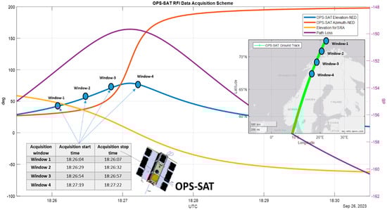
Figure 1.
OPS-SAT operations: Norwegian passage scheduling and data recordings scheme representation including details on the position during the sample recordings used in the analysis.
2.2. Norwegian Jammer Test Coordination Group
Since 2022, the northern shore of Norway, specifically the island of Andøya, has become the world’s largest testing ground for jamming and spoofing, thanks to the Jammertest event. This event is organized by the Norwegian Public Roads Administration (NPRA), Nkom, FFI, Norwegian Metrology Service (JV), and NOSA. Andøya’s location is also somewhat remote, minimizing disruptions to air traffic and normal civilian activities. In this context, the JRC’s team participated in the Jammertest 2023, held between 18 and 22 September, to assess the resilience of GNSS equipment against various types of attacks [6]. The team located on-site coordinated with Norwegian colleagues to set up a high-power jammer, implemented using a reduced configuration of the test setup known as “The Hulk”. As depicted in Figure 2, this setup includes one USRP X410 SDR from Ettus Research, Austin, TX, USA. The exciter output signal is routed to a programmable step attenuator with an attenuation range of 95 dB in 0.25 dB steps. The output from the attenuators is then connected to a power amplifier. The antenna is a directional helical antenna with Right Hand Circular Polarized (RHCP) and 10 dB gain. A PC running Linux controls the high-power jammer, managing both exciters and the step attenuator. The high-power jammer is connected to Internet and synchronized with GPS time using Network Time Protocol (NTP). The chirp signal type was chosen as the most suitable candidate to be generated for the space experiment. The following characteristics have been considered: (i) carrier frequency (1575.42 MHz with a 250 kHz shift); (ii) bandwidth (+/−20 kHz); (iii) sweep time (1 ms); (iv) power (20 W). Figure 2 shows the Power Spectral Density (PSD) of the chirp signal before the transmission.
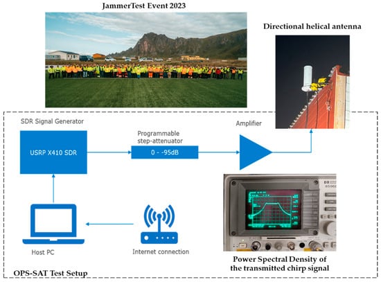
Figure 2.
Jamming signal generation setup for the OPS-SAT experiment during the Norwegian Jammertest, 2023 [5].
3. OPS-SAT SDR Data Processing for Spectrum Monitoring
This section presents signal processing operations applied to the I/Q samples collected from OPS-SAT. Specifically, Figure 3 reports the PSD computed on the I/Q samples retrieved from the recorded telemetries.

Figure 3.
Power Spectral Density computed on four acquisition windows of I/Q samples, collected on 26 September 2023.
It is worth noting that four PSDs are reported on the same figure, i.e., one for each acquisition window. There are different spurious/harmonics, which are always at the same frequencies for all the acquisition windows. In other words, these spurious/harmonics are independent of the satellite movement and of the Doppler shift. Hence, these lines are necessarily introduced by the satellite circuitry and can be filtered away with ad hoc digital filters. Examples of these spurious elements include the spectral lines around −400 kHz, between 0 and 100 kHz, and around 600 kHz.
The jammer signal is clearly visible between 200 and 400 kHz. It is centered at different frequencies for each acquisition window, due to the Doppler shift caused by the LEO satellite motion. Let us remember that the jammer has been transmitted centered at L1 plus 250 kHz. Considering that the OPS-SAT front-end sampled the signal centered at 1.5754 GHz, the jammer would be centered exactly 270 kHz above the 0 frequency in the digital spectrum in absence of Doppler shift and carrier frequency error (due to the receiver crystal). This is in line with what is shown through the PSD analysis, but is better highlighted in Figure 4, which reports an example of spectrograms computed on the I/Q samples collected from OP-SAT.
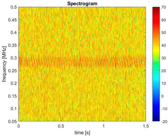
Figure 4.
Spectrogram computed on the I/Q samples collected from OPS-SAT with active chirp jammer (Acquisition window 2, i.e., the one collecting more jammer energy).
This spectrogram is specific for the Acquisition 2, collected (26 September 2023 over Norway at 18:26:29) as reported in Section 2. Similarly, to the PSD analysis, the spectrogram shows the presence of the jammer transmitted from ground and visible in the frequency region between 200 and 400 kHz. It is worth observing that the frequency variation following the chirp profile is visible in the spectrogram, thanks to proper selection of the FFT size. In fact, the inclined red segments represent the saw tooth statement of the instantaneous chirp frequency, matching features of the jammer signal, transmitted from the Jammertest location.
4. Single Satellite Two-Step Geolocation of the On-Ground Emitter
This work assumes a two-step approach for localization, hence time or frequency shift observation obtained from the received signal processing can then be converted into a time series of measurements to feed the emitter geolocation algorithm. A key technique in single-satellite localization of emitters is the FDOA method [7], which locates the interference by calculating the finite variation ΔFOA of the frequency of arrival (FOA) [8]. Therefore, the first step of the emitter localization is based on the generation of FDOA observables, obtained by means of the computation of the Complex Ambiguity Function (CAF), whose theoretical expected accuracies and computational complexity is addressed in [9]. The calculation of the CAF can be considered as the basis for joint estimation of the differential delay and differential frequency offset between two waveforms that contain a common component plus additive noise. This could be the case of two waveforms acquired by two different sensors [3] or two chunks of signal acquired by a unique sensor at different time instants, as for our OPS-SAT case. The FDOA measurements can be obtained by detecting the pair in correspondence of the CAF peak, i.e.,
where and are the complex envelopes of two waveforms that contain a common component, while and are the time lag and the frequency offset to be searched.
It is worth observing that the integration time for the CAF computation has been set equal to 1 ms, whereas the frequency shift domain has been dimensioned by observing the Doppler shift curve for OPS-SAT. In fact, by observing this curve, we can compute the maximum Doppler shift between two time instants separated by 25 s. The example of CAF is reported in Figure 5.
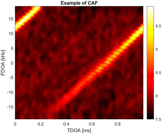
Figure 5.
Example of CAF computed between window 2 and window 3.
Now let us observe that the FDOA approach, which relies on the computation of CAF, generates observables affected by a noise greater than the one embedded in the single acquisition window. However, this is the most viable approach for our experiment, considering the imprecise time and frequency tag of each acquisition window, which may lead to biased observables. Instead, by using a differential approach (based on the CAF), these biases can be mitigated. Now let us focus on the estimation of the SNR for each acquisition window, where with the expression “signal” we refer to the signal from the jammer. The jammer power has been computed by integrating the filtered PSD over the jammer bandwidth, whereas the noise power has been computed by integrating the noise floor over the digital filter bandwidth. The obtained SNR estimations are reported in Table 1.

Table 1.
Effective input and output SNR for each CAF computation.
By using the approach proposed in [9], it is possible to compute the effective input SNR and effective output SNR, basing on the SNR estimated from the acquisition windows collected by OPS-SAT. It is worth noticing that [9] suggests, as rule of thumb, that the effective output SNR should always exceed 10 dB. Considering the effective output SNRs measured for our experiment (see Table 1), which are few dBs above the minimum value of 10 dB, we can figure out that FDOA observables will be noisy, impacting the jammer geolocation accuracy.
The second step is based on mapping FDOA observables at that measurement epoch in the geometric domain in order to localize the emitter. In this case, the measurement model can be expressed as
In (3), incorporates receiver clock offset rate and other residual stationary biases. Instead, represent the measurement noise error introduced by noisy signals involved in the CAF estimation. The measurement model in (2) directly defines the emitter unknown localization as the minimum of the following non-linear estimation problem:
where x = ; represents the final FDOA measurement model including the general model simplification according to emitter position constraints and all reference frame mapping functions; are the known receiver positions provided by the satellite orbit data propagation at time and ; is a proper whitening covariance matrix taking into account measurement noise and residual errors; and is here considered inner bias affecting the estimation problem.
The problem in (4), as per standard FDOA localization approaches, can be prone to multiple minima, so a global search is generally suggested. Different optimizers can be investigated, but a local non-linear least square solver integrated with multiple start approach has been selected as working solution to find the global minima.
5. Experimentation Results
The OPS-SAT experiment scenario introduces several challenges into the localization task. The uncertainties and errors are not limited to those generated by signal processing but also those that directly affect the geometry. Figure 6 summarizes such a localization scenario, where the following issues are identified:

Figure 6.
OPS-SAT geometry limitations.
- Only four chunks (block 1–4 in Figure 6) of data could have been collected (as explained in Section 2.1), lasting 3 s each. This sparse data collection jeopardizes the observability of the whole Doppler dynamic (orange curve).
- Coarse estimation of FOA measurement (green samples) has shown huge biases with respect to the expected Doppler (cyan samples), making FDOA a more robust but potentially less accurate approach.
- The low SNR furthermore reduces the number of usable measurements, requiring some non-coherent combination, leading to 10 FDOA observables for the acquisition window (red samples).
- The failure of the on-board GNSS receiver does not allow the correction of the measurements clock offset rate as per standard FDOA approach [3]. The same GNSS failure introduces uncertainty regarding the OPS-SAT satellite orbit propagation only low accuracy TLE files can be used for the purpose and discrepancies in the measurement time stamps affect the synchronization with the spacecraft positioning.
All those effects shall be considered as worst-case condition for a fine geolocation of the emitter, but they do not make it impossible to provide at least a coarse localization. This is demonstrated by comparing the expected FDOA observations, derived from the known geometry between the transmitter and the satellite, to the raw FDOA extracted from real data processing using CAF. The comparison is presented in the left box-plot of Figure 6, where the estimated and measured values are represented by the red and blue stepwise curves, respectively.
The final result for the emitter localization over the Norwegian test area is provided in Figure 7. The estimated emitter position is indicated by the cyan circle, while the actual target emission location in Andoya is marked with a large white cross. The solution exhibits an error of approximately 40 km in latitude and 70 km in longitude.

Figure 7.
Localization results of the jammer emitter via OPS-SAT experiment.
Figure 7 also shows the localization cost function in terms of orange contour lines over the latitude–longitude region of interest (ROI) . As expected, the error distribution in latitude and longitude reflects the sensing geometry experienced along the satellite’s ground track (indicated by the green line).
The precision is clearly limited by the unknown residual biases that cannot be calibrated and the very high measurement noise (stepwise plot in Figure 6). However, the result confirms the capability to provide coarse detection and localization of the jamming area with limited hardware resources. This is highlighted by the error ellipsoid evaluated in the target solution point from the correspondent 2D latitude and longitude covariance. The ellipsoid is quite large considering the experienced high uncertainty level, but it provides consistent bounds, including the true emission site.
6. Conclusions
This paper presented an experiment in the field of interference detection and geolocation from LEO by leveraging the availability of OPS-SAT operated by ESA ESOC for I/Q sample recording and the opportunity of transmitting high power jammer in GNSS band in the context of Jammertest 2023. The JRC team identified the best satellite passage in the Jammertest area and scheduled the data collection. The FFI team, jointly with JRC members, focused on activating the chirp jammer during the satellite passage. The collection of this jammer data set is a fundamental asset for JRC. Unfortunately, due to OPS-SAT hardware constraints, the recording time was limited to few seconds, limiting the recorded Doppler dynamic related to the satellite movement. However, this paper proposes the use of CAF between disjointed acquisition windows in the time domain to derive the FDOA observables, which are then employed for geolocation purposes. Despite biased and noisy FDOA observables, this paper shows that it is possible to perform a coarse geolocation of the jammer. As remarked throughout the paper, gaining knowledge of the jammer signal waveform and its precise location was a unique opportunity to assess performances and limits in terms of jamming detection and geolocation algorithms. Finally, let us remark that, to the best of author’s knowledge, this is the first data set collection from LEO in L-band performed during the Jammertest event, which could be replicated in the near future, potentially investigating different jammers or even a combination of them, with the idea of gathering a wider understanding of the interference monitoring from space.
Author Contributions
Conceptualization, F.M.; software, O.M.P.; writing—review and editing, T.S., methodology, L.C. and A.P.; resources, V.Z.; project administration, J.F.-G. All authors have read and agreed to the published version of the manuscript.
Funding
This research received no external fundings.
Institutional Review Board Statement
Not applicable.
Informed Consent Statement
Not applicable.
Data Availability Statement
No new data were created or analyzed in this study. Data sharing is not applicable to this article.
Acknowledgments
The authors wish to thank the Norwegian Communication Authority (Nkom) and Norwegian Defense Research Establishment (FFI) for allowing and supporting the execution of the experiment discussed within this paper. The support of ESA is also gratefully acknowledged.
Conflicts of Interest
The authors declare no conflict of interest.
References
- Ellis, P.; Rheeden, D.V.; Dowla, F. Use of Doppler and Doppler Rate for RF Geolocation Using a Single LEO Satellite. IEEE Access 2020, 8, 12907–12920. [Google Scholar] [CrossRef]
- Ellis, P.; Irisov, V.; Pojani, G.; Binda, S.; Khan, H.; Cappaert, J.; Yuasa, T.; Nogues Correig, O. GNSS Interference Monitoring from LEO Using the Spire Constellation; 4S Symposium: Vilamoura, Portugal, 2022. [Google Scholar]
- Clements, Z.; Humphreys, T.E.; Ellis, P. Dual-Satellite Geolocation of Terrestrial GNSS Jammers from Low Earth Orbit. In Proceedings of the 2023 IEEE/ION Position, Location and Navigation Symposium (PLANS), Monterey, CA, USA, 24–27 April 2023; pp. 458–469. [Google Scholar] [CrossRef]
- Mladenov, T.; Fischer, B.; Evans, D. ESA’s OPS-SAT Mission: Powered by GNU Radio. In Proceedings of the 10th GNU Radio Conference, Online, 14–18 September 2020; Volume 5. Available online: https://pubs.gnuradio.org/index.php/grcon/article/view/65 (accessed on 14 March 2025).
- Norwegian Communications Authority. Jammertest 2023—Test Plan. 2023. Available online: https://jammertest.no/content/files/2024/03/Jammertest-2023---Testplan.pdf (accessed on 14 March 2025).
- Broumandan, A.; Pirsiavash, A.; Tremblay, I.; Kennedy, S. Hexagon|NovAtel’s Jamming and Spoofing Detection and Classification Performance During the Norwegian JammerTest 2023. In Proceedings of the 2024 International Technical Meeting of The Institute of Navigation, Long Beach, CA, USA, 23–25 January 2024; pp. 467–480. [Google Scholar] [CrossRef]
- Ho, D.K.C.; Chu, J.C.; Downey, M.L. Determining Transmit Location of an Emitter Using a Single Geostationary Satellite. U.S. Patent US8,462,044B1, 11 June 2013. [Google Scholar]
- Kalantari, A.; Maleki, S.; Chatzinotas, S.; Ottersten, B. Frequency of arrival-based interference localization using a single satellite. In Proceedings of the 2016 8th Advanced Satellite Multimedia Systems Conference and the 14th Signal Processing for Space Communications Workshop (ASMS/SPSC), Palma de Mallorca, Spain, 5–7 September 2016; pp. 1–6. [Google Scholar] [CrossRef]
- Stein, S. Stein Algorithms for ambiguity function processing. IEEE Trans. Acoust. Speech Signal Process. 1981, 29, 588–599. [Google Scholar] [CrossRef]
Disclaimer/Publisher’s Note: The statements, opinions and data contained in all publications are solely those of the individual author(s) and contributor(s) and not of MDPI and/or the editor(s). MDPI and/or the editor(s) disclaim responsibility for any injury to people or property resulting from any ideas, methods, instructions or products referred to in the content. |
© 2025 by the authors. Licensee MDPI, Basel, Switzerland. This article is an open access article distributed under the terms and conditions of the Creative Commons Attribution (CC BY) license (https://creativecommons.org/licenses/by/4.0/).