An Experimental Study for Localization Using Lidar Point Cloud Similarity

Abstract

In this paper, we consider the use of high-definition maps for autonomous vehicle (AV) localization. An autonomous vehicle may have a variety of sensors, including cameras, lidars, and Global Positioning System(GPS) sensors. Each sensor technology has its own pros and cons; for example, GPS may not be very effective in a city environment with high-rise buildings; cameras may not be very effective in poorly illuminated environments; and lidars simply generate a relatively dense local point cloud. In a typical autonomous vehicle system, all of these sensors are present and sensor fusion algorithms are used to extract the most accurate information. Using our AV research vehicle, we drove on our university campus and recorded Real Time Kinematic-GPS(RTK-GPS) (ZED-F9P) and Velodyne Lidar (VLP-16) data in a time-synchronized fashion. In other words, for every GPS location on our campus, we have lidar-generated point cloud data, resulting in a simple high-definition map of the campus. The main challenge that we look to overcome in this paper is thus: given a high-definition map of the environment and local point cloud data generated by a single lidar scan, determine the AV research vehicle’s location by using point cloud “similarity” metrics. We first propose a computationally simple similarity metric and then describe a recursive Kalman filter-like approach for localization. The effectiveness of the proposed similarity metric has been demonstrated using the experimental data.

1. Introduction

Localization is a critical challenge in autonomous vehicle navigation [1]. In this paper, we propose a high-definition (HD) map-based approach to enhancing localization accuracy. The HD map is a directed graph of GPS coordinates linked to lidar scans and can be expanded with sensor data, such as cameras and radar, for greater detail [2,3]. The core issue addressed is whether a lidar-generated point cloud, combined with similarity metrics, can accurately determine the vehicle’s location. We assert that this is feasible using computationally efficient algorithms, while human drivers often rely on visual matching to locate themselves, computer-based visual matching offers unique advantages and challenges. Our focus here is on lidar point cloud matching [4]. Lidar output consists of three-dimensional point sets, which are generally considered more computationally tractable than processing color images. This research builds on our previous work [5,6,7], funded by National Science Foundation(NSF) and Florida Polytechnic University. Using our autonomous vehicle platform, we collected over 30 min of synchronized lidar scans and GPS coordinates during campus-wide driving. This dataset is employed to validate the proposed point cloud matching algorithms, similarity metrics, and localization methods.

2. Data Collection

A point cloud is defined as a finite set of points in ${\mathbb{R}}^3$; namely, any set of the following form is a point cloud:

$$P=\{x_k:x_k\in {\mathbb{R}}^3,k=0,\cdots ,N-1\}$$

In an AV application, the lidar sensor output will be a point cloud. Even though the point $x_k$ can be indexed by an integer, any permutation will result in the same point cloud object. Furthermore, even if these points are stored in an array-like structure, with each point having an index (e.g., a list or matrix), we still consider the point cloud to be a set.

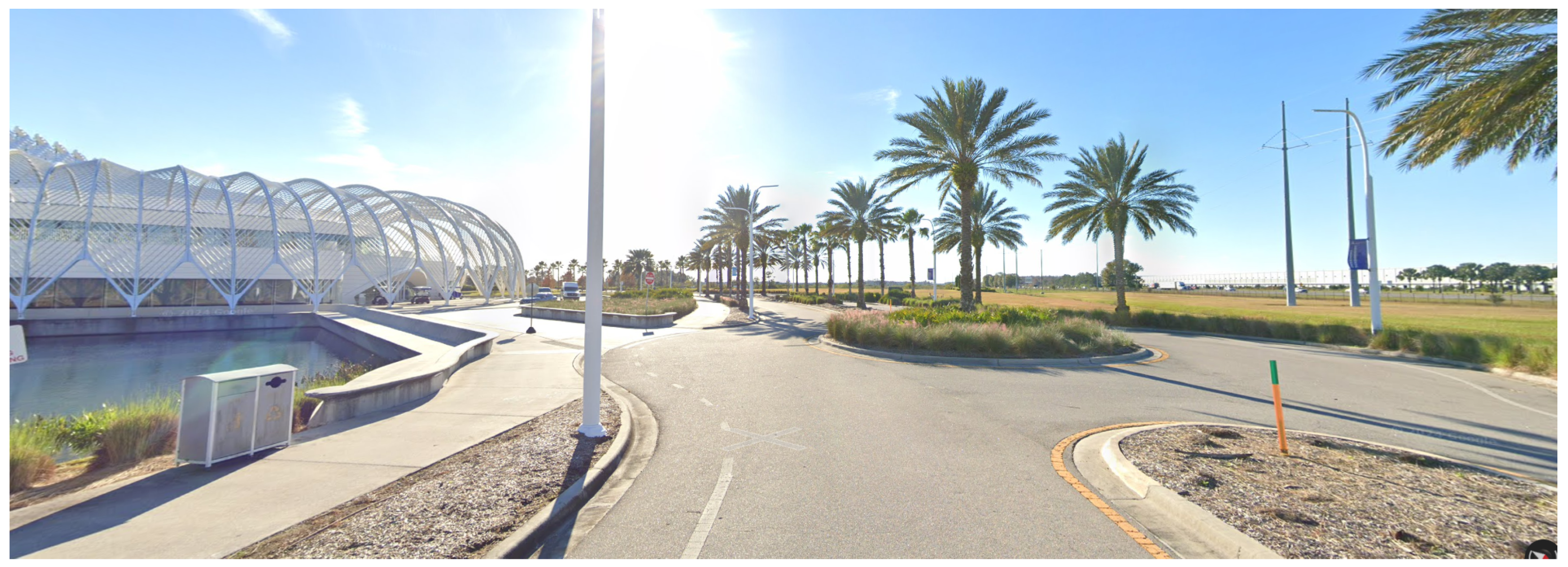
An example point cloud is shown in Figure 1, and the Google street view of a nearby location is shown in Figure 2. This is the entrance of the Innovation Science and Technology (IST) building at Florida Polytechnic University.

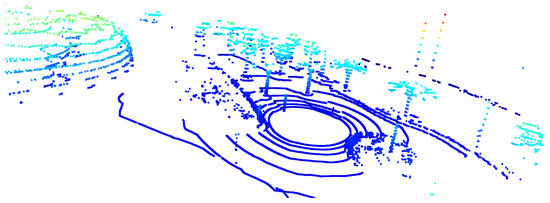
Figure 1. Point cloud obtained from our Velodyne VLP-16 lidar sensor.

Figure 2. Google Street View of a nearby location.

The point cloud shown in Figure 1 is one of our 19,500 point clouds collected while we drove on the Florida Poly campus using our AV research vehicle. This particular point cloud consists of 18,165 three-dimensional vectors; in other words, it can be stored as a 18,165 $\times 3$ real-valued matrix. The three-dimensional (3D) visualization shown in Figure 1 was generated using the Python Open3D library.

Almost all of the 19,500 point clouds have a different number of points. In Figure 3, a histogram of the number of points is shown. We see that the mean value of the number of points is 21,533 and the standard deviation is 1685 points. The Velodyne VLP-16 lidar sensor used in this application has 16 lasers, each scanning a different polar angle. In this study, a 360-degree lidar scan was completed in 0.1 s; in other words, the lidar frame rate was 10 fps.

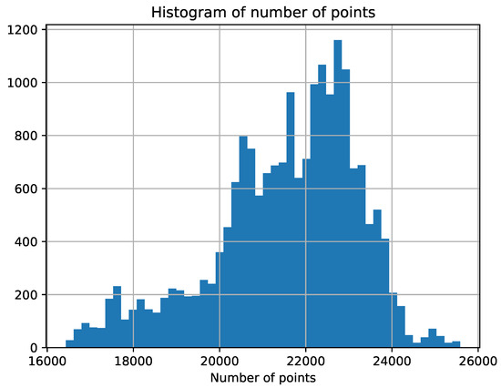
Figure 3. Histogram of the number of points in our point clouds.

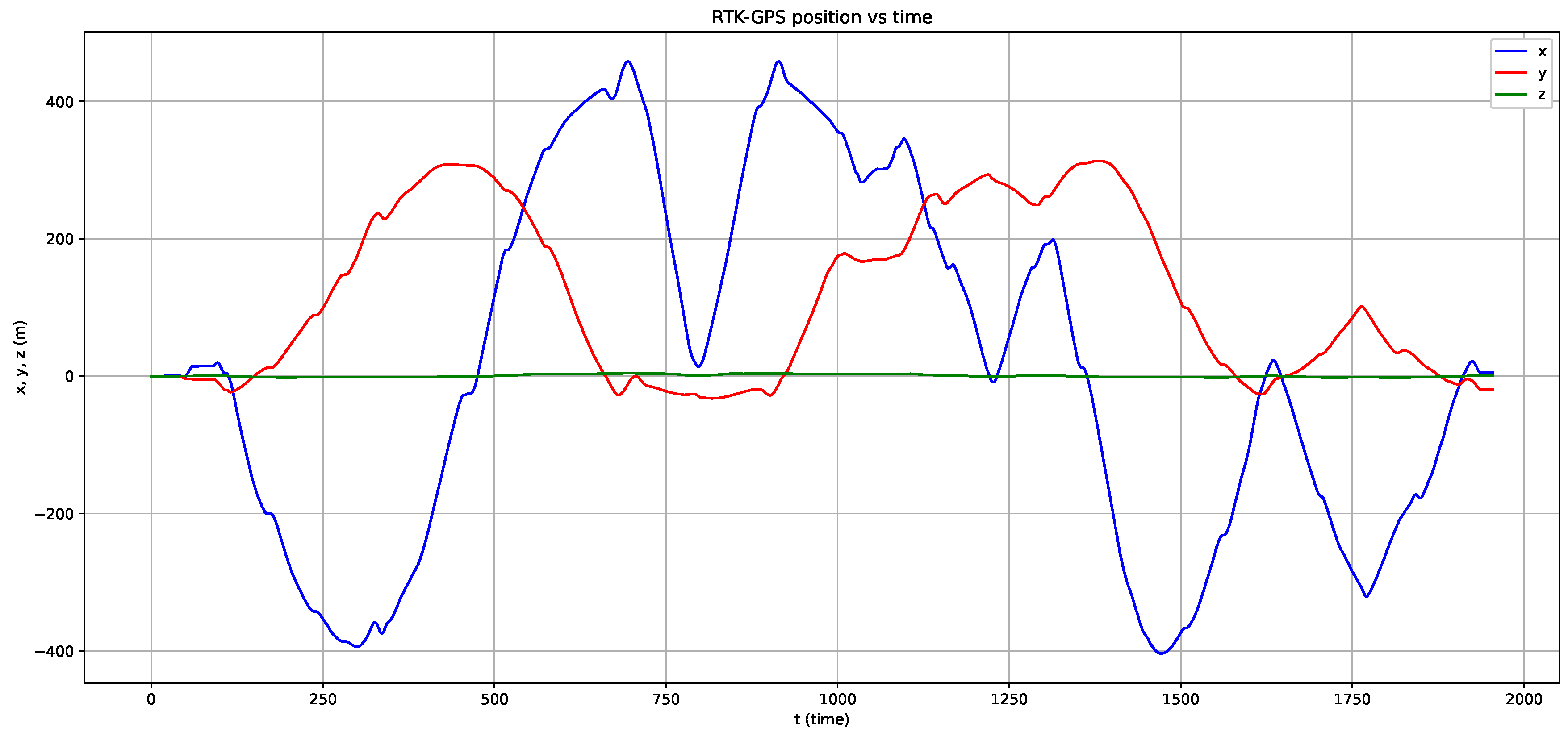
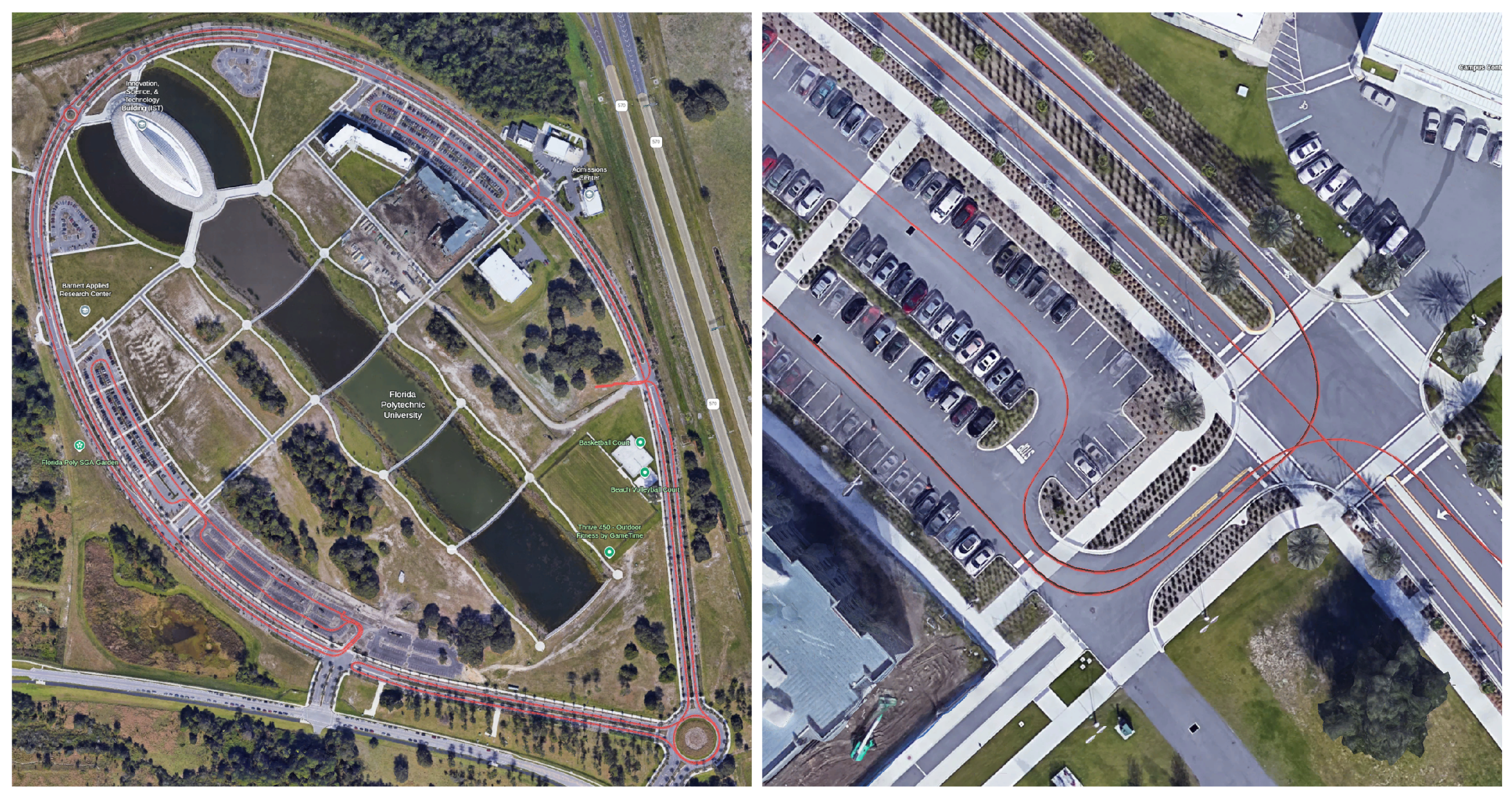
While driving on the Florida Poly campus, we also recorded our AV research vehicle’s GPS location using an RTK-GPS. The particular RTK-GPS system used in this study comprised the ublox ZED-F9P sensor and the C099-F9P application board. The RTK-GPS output rate was set to 2 Hz, and Florida Department of Transportation’s (FDOT) Florida Primary Reference Network was used as base stations. In Figure 4, the path followed by our AV research vehicle is shown in Cartesian coordinates, and the origin is a point close to the newly constructed Barnett Applied Research Center(BARC). The “map” view is shown in Figure 5. The RTK-GPS output is basically in text format, as described in the National Marine Electronics Association(NMEA) 0183 standard. If this is saved in KMZ format, it can be viewed on Google Earth, as shown in Figure 5.

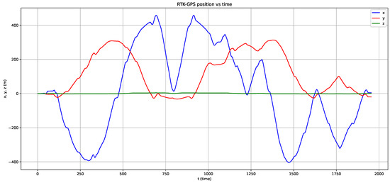
Figure 4. The path followed by our AV research vehicle in Cartesian coordinates, i.e., $\left(x\right(t),y(t),z(t\left)\right)$ versus t. The starting point is a point close to the BARC Applied Research Center.

Figure 5. The path followed by our AV research vehicle shown in Google Earth.

The data collection process took approximately 1950 s, a little over half an hour. In the end, we had several lidar point clouds and RTK-GPS location measurements, as follows:

$$P_k,g_{k}k=0,\cdots ,N-1$$

where N = 19,500, $P_k$’s are point clouds, and $g_k$’s are the location tags as three dimensional vectors. Since the RTK-GPS frame rate is 2 fps and the lidar frame rate is 10 fps, we first synchronized the clocks of these two sensors and then interpolated the RTK-GPS data by a factor of 5 to transform it into a 10 fps rate.

3. Point Cloud Similarity Metrics

In this section, we will consider the problem of measuring the similarity between two point clouds. If $P_1$ and $P_2$ are two-point clouds, and if it is possible to find a translation vector $v_T\in {\mathbb{R}}^3$ and a rotation matrix $R\in \mathrm{SO}\left(3\right)$, such that the following significantly overlaps:

$$P_1,\mathrm{and}R{P}_2+v_T$$

then, it is reasonable to call $P_1$ and $P_2$ as similar. In other words, one can say that $P_1$ and $P_2$ match. The main idea behind this lidar-based localization is point cloud similarity or matching. Defining an unambiguous and computationally simple method is of extreme importance.

Since rotations do not change the center of mass of the point cloud, without a loss of generality, we may assume that point clouds have their centers already aligned. To measure the degree of overlap, we propose the use of a distance metric defined for point clouds. Therefore, if $\mathrm{dist}$ is a measure of distance between two point clouds, our proposed similarity metric will be as follows:

$$\mathrm{sim}(P_1,P_2)=\underset{R\in \mathrm{SO}\left(3\right)}{min}\mathrm{dist}(P_1,R{P}_2)$$

Because of the already assumed center of mass alignment between $P_1$ and $P_2$, we drop the $v_T$ term. In this equation, $\mathrm{SO}\left(3\right)$ represents the set of rotation matrices.

In the literature, there are various point cloud distance metrics used, such as Chamfer distance, Hausdorff distance, one-sided Hausdorff distance, and Sinkhorn distance. In this study, we adopt the Chamfer distance, which is defined as follows:

$$\mathrm{dist}(P_1,P_2)={\displaystyle \frac{1}{2N_1}}\sum _{i=0}^{N_1-1}|u_i-NN(u_i,P_2)|+{\displaystyle \frac{1}{2N_2}}\sum _{j=0}^{N_2-1}|v_j-NN(w_j,P_1)|$$

where $P_1$ is the point cloud $\{u_0,\cdots ,u_{N_1-1}\}$, consisting of $N_1$ three dimensional points, and $P_2$ is the point cloud $\{v_0,\cdots ,v_{N_2-1}\}$, consisting of $N_2$ three dimensional points. The function $NN$ is called the nearest neighbor function and is defined as follows:

$$NN(x,P)=arg\underset{y\in P}{min}{\parallel x-y\parallel }_2,$$

where ${\parallel ·\parallel }_2$ is the Euclidean distance. In other words, $NN(x,P)$ is the point in the point cloud P that is closest to x in Euclidean distance.

4. A Simplified Similarity Metric

One problem with the “ideal” similarity definition given in the previous section is the complexity of the search over SO(3) and the computational costs associated with Chamfer distance. Since our point clouds have around $N=$ 20,000 points, the computation of the $NN$ function will require a for loop of size N. The Chamfer distance formula has a sum over N as well, i.e., another for loop of size N. On top of all of this, we have a search over SO(3), i.e., a two-dimensional search over $[0,2\pi )\times [0,2\pi )$.

If the AV vehicle is traveling at higher speeds, we have a very short time interval in which to finish all localization calculations. Therefore, we would like to propose less “ideal” but computationally simpler similarity metrics that are likely to result in similar matching scores.

First, consider each point cloud in spherical coordinates, as follows:

$$P=\{(r_k,{\theta }_k,{\varphi }_k):k=0,\cdots ,N-1\},$$

Then, drop the radius info and generate the following set of two-dimensional points:

$$Q=\{({\theta }_k,{\varphi }_k):k=0,\cdots ,N-1\}.$$

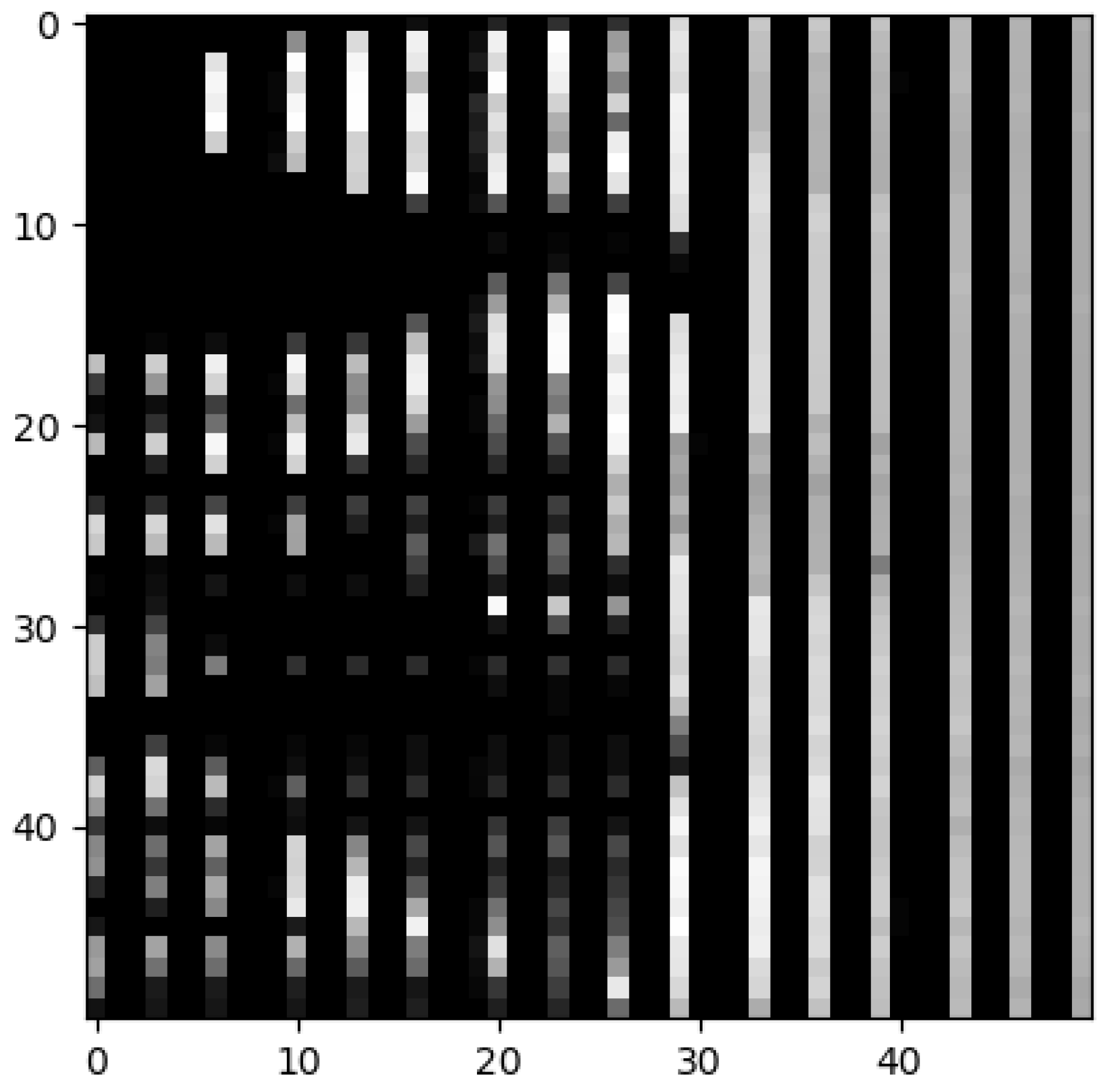
Dropping the radius info will result in some loss of information, but greatly simplifies the whole process. Then, consider the two-dimensional (2D) histogram of this set Q, which will be effectively a matrix, H, of size $b\times b$, where b is the bin size used in 2D histogram generation. For a typical $b=$ 50–100, the resulting $b\times b$ matrix can be viewed as an image. For example, for the lidar scan shown in Figure 1, histogram analysis will result in the image shown in Figure 6.

Figure 6. Image visualization of the 2D histogram of the point cloud shown in Figure 1.

Rotations of a point cloud P correspond to translations in the Q representation. Since we are using the spherical coordinate system, all translations are modulo $2\pi$ in the first and the second coordinates. If we have two point clouds, $P_1$ and $P_2$, instead of using the similarity metric defined in the previous section, we use the following:

$$\underset{k,\ell }{max}\sum _{i,j}{H}_1[i,j]H_2[i+k,j+\ell ]$$

This can be used as a computationally simpler but not necessarily equivalent alternative. Note that all H matrix indices are considered as modulo b. The double summation used in the above equation is the well-known correlation formula commonly used in image processing. To capture all possible rotations, we allow row and column circular shifts and choose the maximum possible value as the similarity score. The double summation, as a function of $k,\ell$, can be computed using Fast Fourier Transform(FFT) techniques.

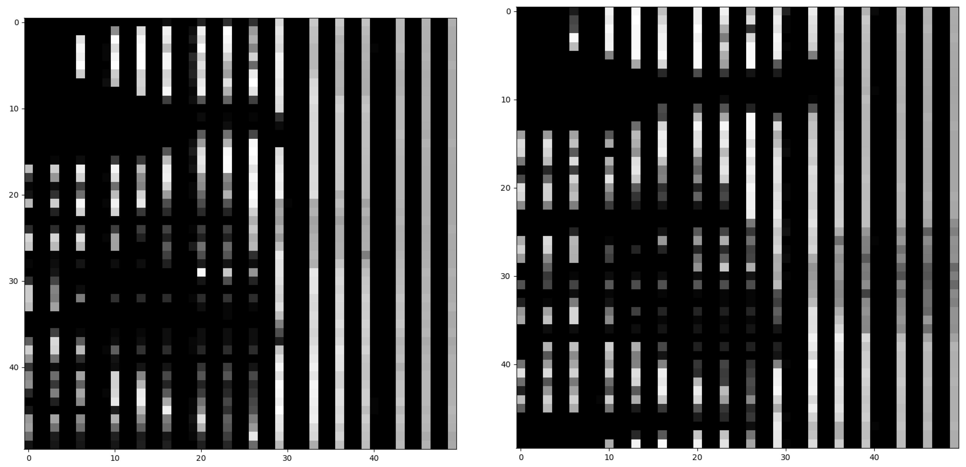
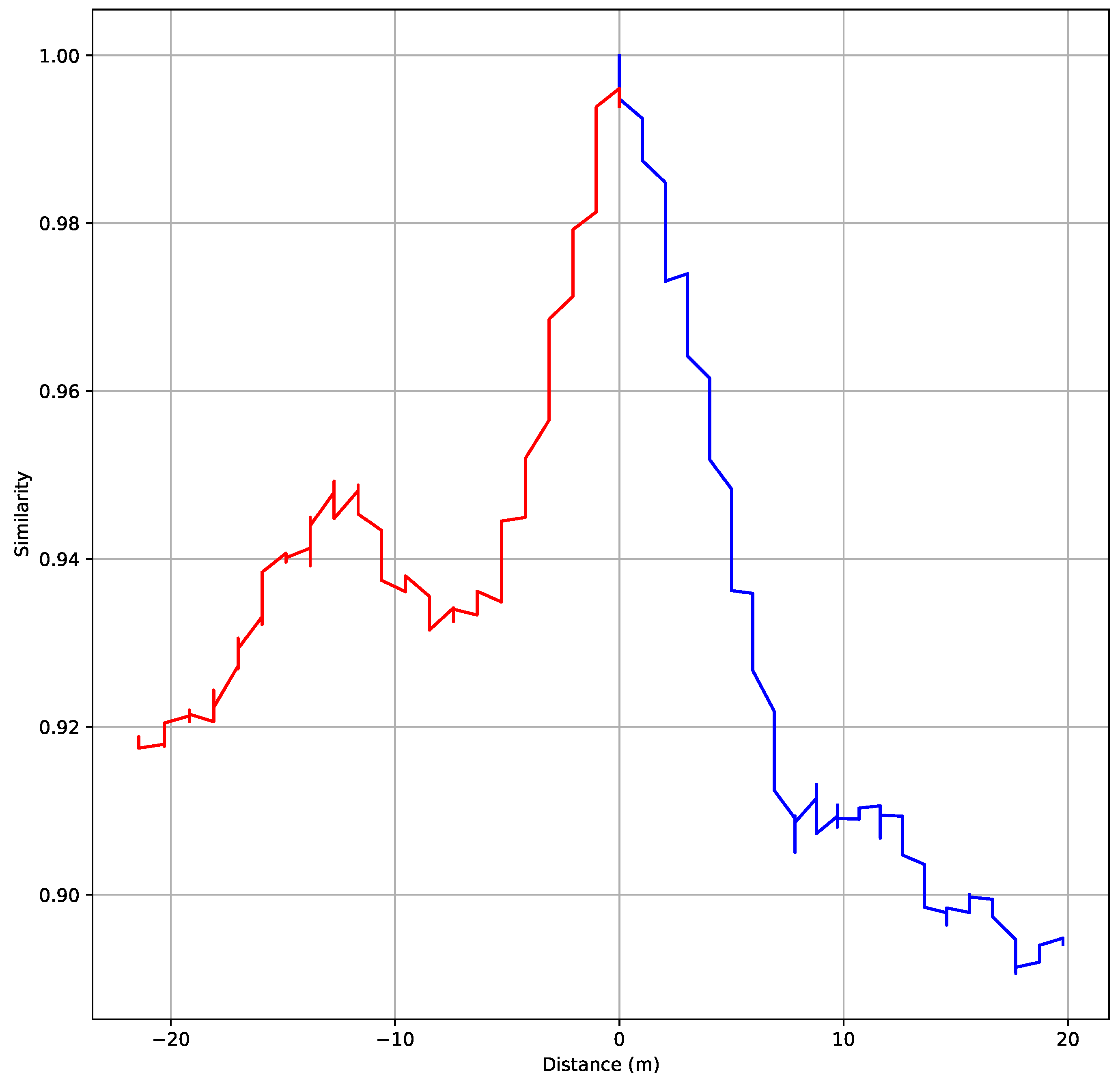
In Figure 7, the image representations of two point clouds are shown. The one on the left is for the 4000th point cloud, and the one on the right is for the $4050\mathrm{th}$ point cloud. Figure 8 shows how the newly defined similarity changes with the distance. It is clear that, as we move away from the point corresponding to the $4000\mathrm{th}$ lidar scan, or the location at time $t=40$, the similarity between the $4000\mathrm{th}$ lidar scan and the lidar scan at the new location drops sharply.

Figure 7. Image representation of two point clouds captured 5 s apart, $t=40$ and $t=45$.

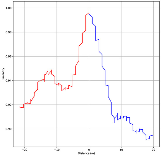
Figure 8. Similarity vs. distance plot at time $t=40$ s.

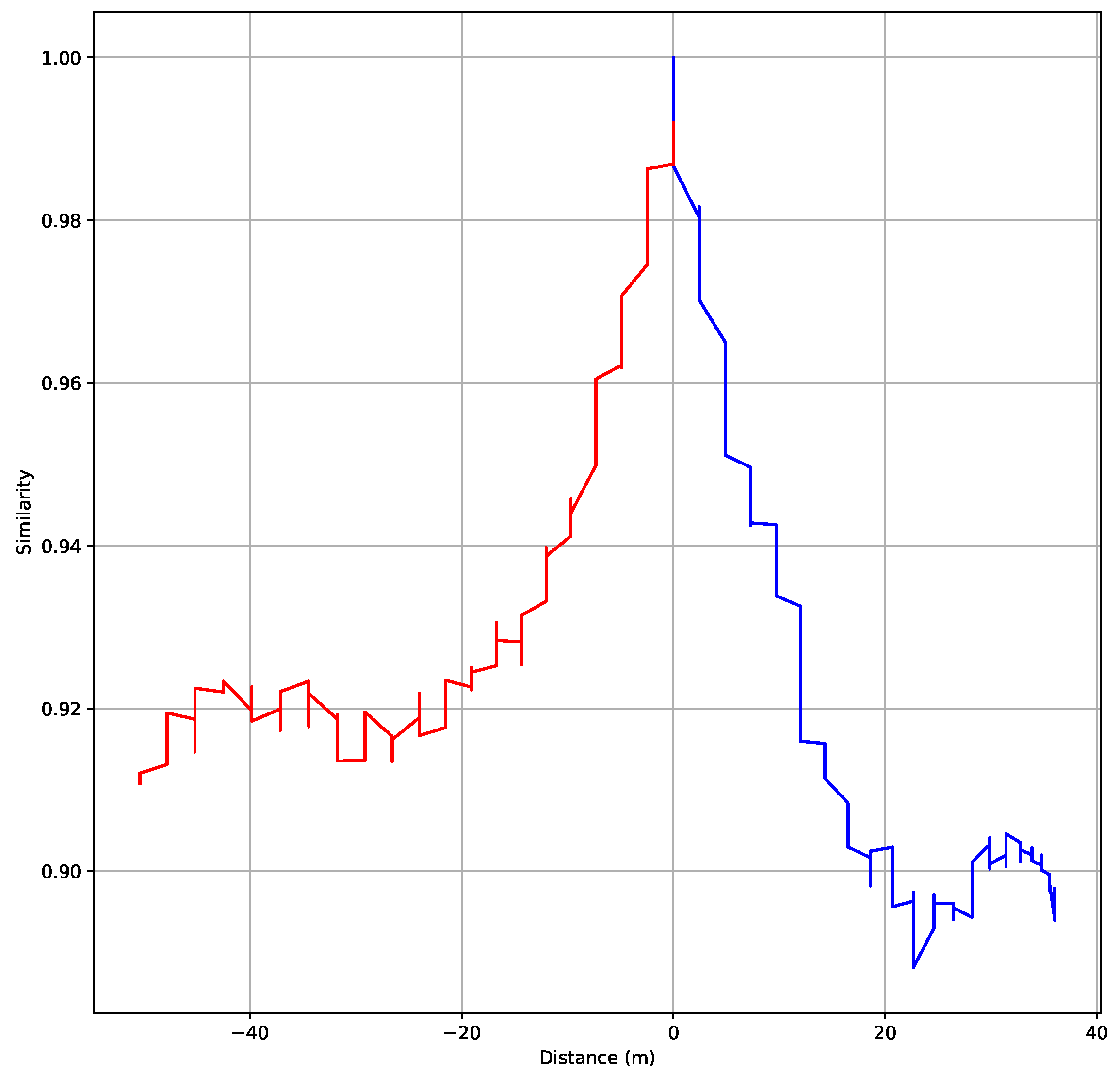
Let us perform the same analysis at time $t=90$. In Figure 9, the image representations of two point clouds are shown. The one on the left is for the $9000\mathrm{th}$ point cloud, and the one on the right is for the $9050\mathrm{th}$ point cloud. Figure 10 shows how the newly defined similarity changes with the distance. It is clear that, as we move away from the point corresponding to the $9000\mathrm{th}$ lidar scan, or the location at time $t=90$, the similarity between the $9000\mathrm{th}$ lidar scan and the lidar scan at the new location drops sharply.

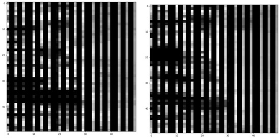
Figure 9. Image representation of two point clouds captured 5 s apart, $t=90$ and $t=95$.

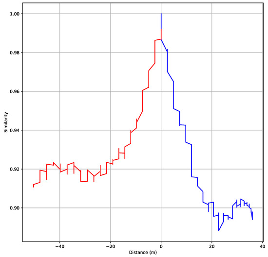
Figure 10. Similarity vs. distance plot at time $t=90$ s.

Proposed Localization Approach

The analysis presented above clearly shows the feasibility of a two-dimensional binary search type approach for localization. We assume that we do know our current location and we assume that, after 1 s, we obtain a new lidar scan. By using this new lidar scan and the proposed similarity scoring methodology, we can update our location. Among all the possible locations that can be reached within 1 s, we choose the location that results in the maximum similarity. More formally, we can write the following:

S1:

Start with $k=0$, and a known current location, $g_k\in {\mathbb{R}}^3$.

S2:

After 1 s, obtain a new lidar scan, $P_{k+1}$.

S3:

Let $S_k=\{g_{\ell }^{\prime }:\ell =0,\cdots ,N_k-1\}$ be the set of all possible GPS locations in the high-definition map that can be reached from $g_k$ within 1 s.

S4:

Let ${\mathcal{P}}_k$ be the set of lidar point clouds for the GPS locations in $S_k$. Recall that the database that maps a GPS location to a point cloud will be called the high-definition map.

S5:

Find the point cloud in ${\mathcal{P}}_k$ that is the most similar to $P_k$.

S6:

Update $g_{k+1}$ as the GPS location corresponding to the point cloud found in Step 5.

S7:

Increase k by 1, and go to Step 2.

5. Conclusions

Using our AV vehicle, we drove on our campus for more than 30 min and saved lidar scans and GPS coordinates. All of this experimental data was used to test the effectiveness of the proposed point cloud matching algorithms, similarity metrics, and localization. Our experimental results show that the proposed approach is computationally simple and effective. The proposed localization approach is recursive and is based on the high-definition map approach outlined in this work. In future work, we plan to explore alternative similarity metrics and compare their performances.

References

- Chalvatzaras, A.; Pratikakis, I.; Amanatiadis, A.A. A Survey on Map-Based Localization Techniques for Autonomous Vehicles. IEEE Trans. Intell. Veh. 2023, 8, 1574–1596. [Google Scholar] [CrossRef]
- Liu, R.; Wang, J.; Zhang, B. High Definition Map for Automated Driving: Overview and Analysis. J. Navig. 2020, 73, 324–341. [Google Scholar] [CrossRef]
- Zang, A.; Li, Z.; Doria, D.; Trajcevski, G. Accurate vehicle self-localization in high definition map dataset. In Proceedings of the 1st ACM SIGSPATIAL Workshop on High-Precision Maps and Intelligent Applications for Autonomous Vehicles (AutonomousGIS ’17), Redondo Beach, CA, USA, 7–10 November 2017; Association for Computing Machinery: New York, NY, USA, 2017. Article 2. pp. 1–8. [Google Scholar]
- Huang, J.; You, S. Point cloud matching based on 3D self-similarity. In Proceedings of the 2012 IEEE Computer Society Conference on Computer Vision and Pattern Recognition Workshops, Providence, RI, USA, 16–21 June 2012; pp. 41–48. [Google Scholar]
- Vargas, J.; Alsweiss, S.; Toker, O.; Razdan, R.; Santos, J. An Overview of Autonomous Vehicles Sensors and Their Vulnerability to Weather Conditions. Sensors 2021, 21, 5397. [Google Scholar] [CrossRef] [PubMed]
- Toker, O. Experimental Performance Analysis of a Self-Driving Vehicle Using High-Definition Maps. In Proceedings of the IEEE Southeast Conference 2023, Orlando, FL, USA, 14–16 April 2023; pp. 565–570. [Google Scholar]
- DeCicco, M.; Khalghani, R.; Toker, O. Drive-By-Wire Conversion of an Electric Golf-Cart for Self-Driving Vehicles Research. In Proceedings of the IEEE Southeast Conference 2023, Orlando, FL, USA, 13–16 April 2023; pp. 724–725. [Google Scholar]
Disclaimer/Publisher’s Note: The statements, opinions and data contained in all publications are solely those of the individual author(s) and contributor(s) and not of MDPI and/or the editor(s). MDPI and/or the editor(s) disclaim responsibility for any injury to people or property resulting from any ideas, methods, instructions or products referred to in the content. |
© 2024 by the authors. Licensee MDPI, Basel, Switzerland. This article is an open access article distributed under the terms and conditions of the Creative Commons Attribution (CC BY) license (https://creativecommons.org/licenses/by/4.0/).