On the Adaptive Numerical Solution to the Darcy–Forchheimer Model ^†

Abstract

We considered a primal-mixed method for the Darcy–Forchheimer boundary value problem. This model arises in fluid mechanics through porous media at high velocities. We developed an a posteriori error analysis of residual type and derived a simple a posteriori error indicator. We proved that this indicator is reliable and locally efficient. We show a numerical experiment that confirms the theoretical results.

1. Introduction

The Darcy–Forchheimer model constitutes an improvement of the Darcy model which can be used when the velocity is high [1]. It is useful for simulating several physical phenomena, remarkably including fluid motion through porous media, as in petroleum reservoirs, water aquifers, blood in tissues or graphene nanoparticles through permeable materials. Let $\Omega$ be a bounded, simply connected domain in ${\mathbb{R}}^2$ with a Lipschitz-continuous boundary $\partial \Omega$. The problem reads as follows: given known functions $\mathbf{g}$ and f, find the velocity $\mathbf{u}$ and the pressure p such that

$$\left\{\begin{array}{ccc}\hfill {\displaystyle \frac{\mu }{\rho }{K}^{-1}\mathbf{u}+\frac{\beta }{\rho }\left|\mathbf{u}\right|\mathbf{u}+\nabla p}& =& \mathbf{g}\mathrm{in}\Omega ,\hfill \\ \hfill \nabla ·\mathbf{u}& =& f\mathrm{in}\Omega ,\hfill \\ \hfill \mathbf{u}·\mathbf{n}& =& 0\mathrm{on}\partial \Omega ,\hfill \end{array}\right.$$

(1)

where $\mu$ is the dynamic viscosity, $\rho$ denotes the fluid density, $\beta$ is the Forchheimer number K denotes the permeability tensor, $\mathbf{g}$ represents gravity, f is compressibility, and $\mathbf{n}$ is the unit outward normal vector to $\partial \Omega$.

We make use of the finite element method to approximate the solution of problem (1). We present the approach by Girault and Wheeler [1], who introduced the primal formulation, in which the term $\nabla ·\mathbf{u}$ undergoes weakening by integration by parts. It is shown in [1] that problem (1) has a unique solution in the space $X\times M$, where $X:={\left[L^3(\Omega )\right]}^2$ and $M:=W^{1,3/2}(\Omega )\cap L_0^2(\Omega )$ (we use the standard notations for Lebesgue and Sobolev spaces).

2. Discrete Problem

To pose a discrete problem, we can use a family ${\left\{{\mathcal{T}}_h\right\}}_{h>0}$ of conforming triangulations to divide the domain $\overline{\Omega }$ such that $\overline{\Omega }={\bigcup }_{T\in {\mathcal{T}}_h}T,\forall h,$ where $h>0$ represents the mesh size. Here we follow [2] and choose the following conforming discrete subspaces of X and M, respectively:

$$\begin{array}{c}{X}_h:=\left\{{\mathbf{v}}_h\in {\left[L^2(\Omega )\right]}^2;\forall T\in {\mathcal{T}}_h,{\mathbf{v}}_h{|}_T\in {\left[{\mathbb{P}}_0\left(T\right)\right]}^2\right\}\subset X,\\ M_h:=Q_h^1\cap L_0^2(\Omega )\subset M,\end{array}$$

where $Q_h^1:=\left\{q_h\in {\mathcal{C}}^0\left(\overline{\Omega }\right);\forall T\in {\mathcal{T}}_h,q_h{|}_T\in {\mathbb{P}}_1\left(T\right)\right\}.$

Then, the discrete problem consists in finding $({\mathbf{u}}_h,p_h)\in X_h\times M_h$ such that

$$\left\{\begin{array}{ccc}\hfill {\displaystyle {\int }_{\Omega }\left(\frac{\mu }{\rho }{K}^{-1}{\mathbf{u}}_h+\frac{\beta }{\rho }\left|{\mathbf{u}}_h\right|{\mathbf{u}}_h\right)·{\mathbf{v}}_{h}dx+{\int }_{\Omega }\nabla p_h·{\mathbf{v}}_{h}dx}& =& {\displaystyle {\int }_{\Omega }\mathbf{g}·{\mathbf{v}}_{h}dx,\forall {\mathbf{v}}_h\in X_h,}\hfill \\ \hfill {\displaystyle {\int }_{\Omega }\nabla q_h·{\mathbf{u}}_{h}dx}& =& {\displaystyle -{\int }_{\Omega }{q}_{h}fdx,\forall q_h\in M_h.}\hfill \end{array}\right.$$

(2)

It is shown in [2] that problem (2) has a unique solution and that the sequence ${\left\{({\mathbf{u}}_h,p_h)\right\}}_h$ converges to the exact solution of problem (1) in $X\times M$. Furthermore, under additional regularity assumptions on the exact solution, some error estimates were derived in [2].

3. Novel Error Estimator and Adaptive Algorithm

We denote by ${\mathcal{E}}_{\Omega }$, ${\mathcal{E}}_{\partial \Omega }$ and ${\mathcal{E}}_T$, respectively, the sets of edges e belonging to the interior domain, the boundary and the element T; $h_e$ denotes the length of a particular edge e; and $h_T$ is the diameter of a given element T. We denote by ${\mathbb{J}}_e\left(v\right)$ the jump of v across the edge e in the direction of ${\mathbf{n}}_e$, a fixed normal vector to side e. Finally, we use the operator $\tilde{\mathcal{A}}({\mathbf{u}}_h,p_h):=\frac{\mu }{\rho }{K}^{-1}{\mathbf{u}}_h+\frac{\beta }{\rho }\left|{\mathbf{u}}_h\right|{\mathbf{u}}_h+\nabla p_h-\mathbf{g}$.

On every triangle $T\in {\mathcal{T}}_h$, we propose the following a posteriori error indicator:

$$\begin{array}{ccc}& {\displaystyle {\theta }_T=(h_T^2\left|\right|\tilde{\mathcal{A}}({\mathbf{u}}_h,p_h){\left|\right|}_{{\left[L^2\left(T\right)\right]}^2}^2+\left|\right|\nabla ·{\mathbf{u}}_h-{f\left|\right|}_{L^2\left(T\right)}^2+\frac{1}{2}\sum _{e\in {\mathcal{E}}_{\Omega }\cap \partial T}{h}_T^{-1}\left|\right|{\mathbb{J}}_e({\mathbf{u}}_h·\mathbf{n}){\left|\right|}_{L^2\left(e\right)}^2}& {\displaystyle +\sum _{e\in {\mathcal{E}}_{\partial \Omega }\cap \partial T}{h}_T^{-1}\left|\right|{\mathbf{u}}_h·\mathbf{n}{\left|\right|}_{L^2\left(e\right)}^2{)}^{1/2}}\hfill \end{array}$$

We also define the global a posteriori error indicator ${\displaystyle \theta :={\left(\sum _{T\in {\mathcal{T}}_h}{\theta }_T^2\right)}^{1/2}}$.

Theorem 1.

For the primal-mixed method (2), there exists a positive constant $C_1$, independent of h, and a positive constant $C_2$, independent of h and T, such that

$$\left|\right|(\mathbf{u}-{\mathbf{u}}_h,p-p_h){\left|\right|}_{X\times M}\le C_1\theta ,$$

$${\theta }_T\le C_2\left|\right|(\mathbf{u}-{\mathbf{u}}_h,p-p_h){\left|\right|}_{{\left[L^3\left(w_T\right)\right]}^2\times W^{1,3/2}\left(w_T\right)},\forall T\in {\mathcal{T}}_h,$$

where $w_T={\bigcup }_{{\mathcal{E}}_T\cap {\mathcal{E}}_{T^{\prime }}\ne }{T}^{\prime }$.

We propose an adaptive algorithm based on the a posteriori error indicator $\theta$. Given an initial mesh, we follow the iterative procedure described in Figure 1. Each new mesh is generated as suggested in [3].

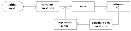
Figure 1. Adaptive algorithm flux diagram.

4. Numerical Experiment

We performed several simulations in FreeFem++ [4], validating the theoretical results. Here we select an example on an L-shaped domain, $\Omega ={(-1,1)}^2{[0,1]}^2$, and focus on the data f and $\mathbf{g}$ so that the exact solution is

$$p(x,y)=\frac{1}{x-1.1},\mathbf{u}(x,y)=\left(\begin{array}{c}exp\left(x\right)sin\left(y\right)\\ exp\left(x\right)cos\left(y\right)\end{array}\right).$$

(3)

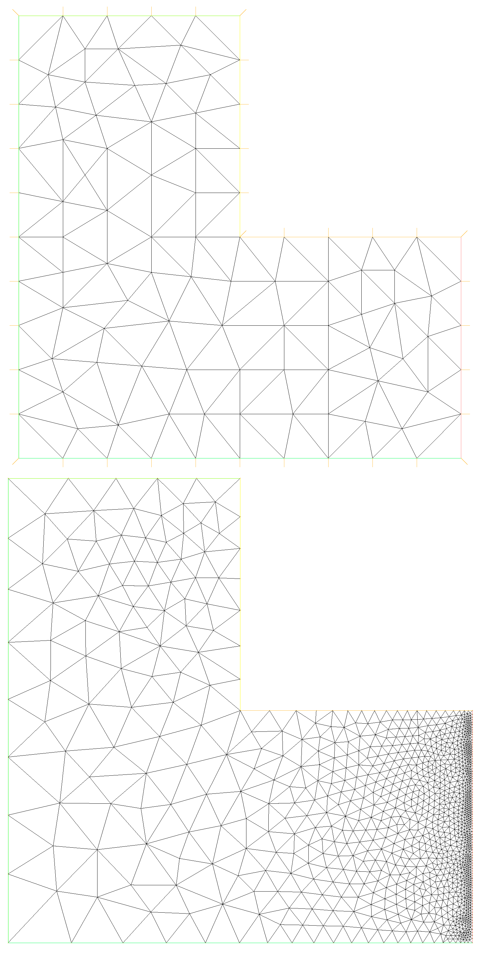
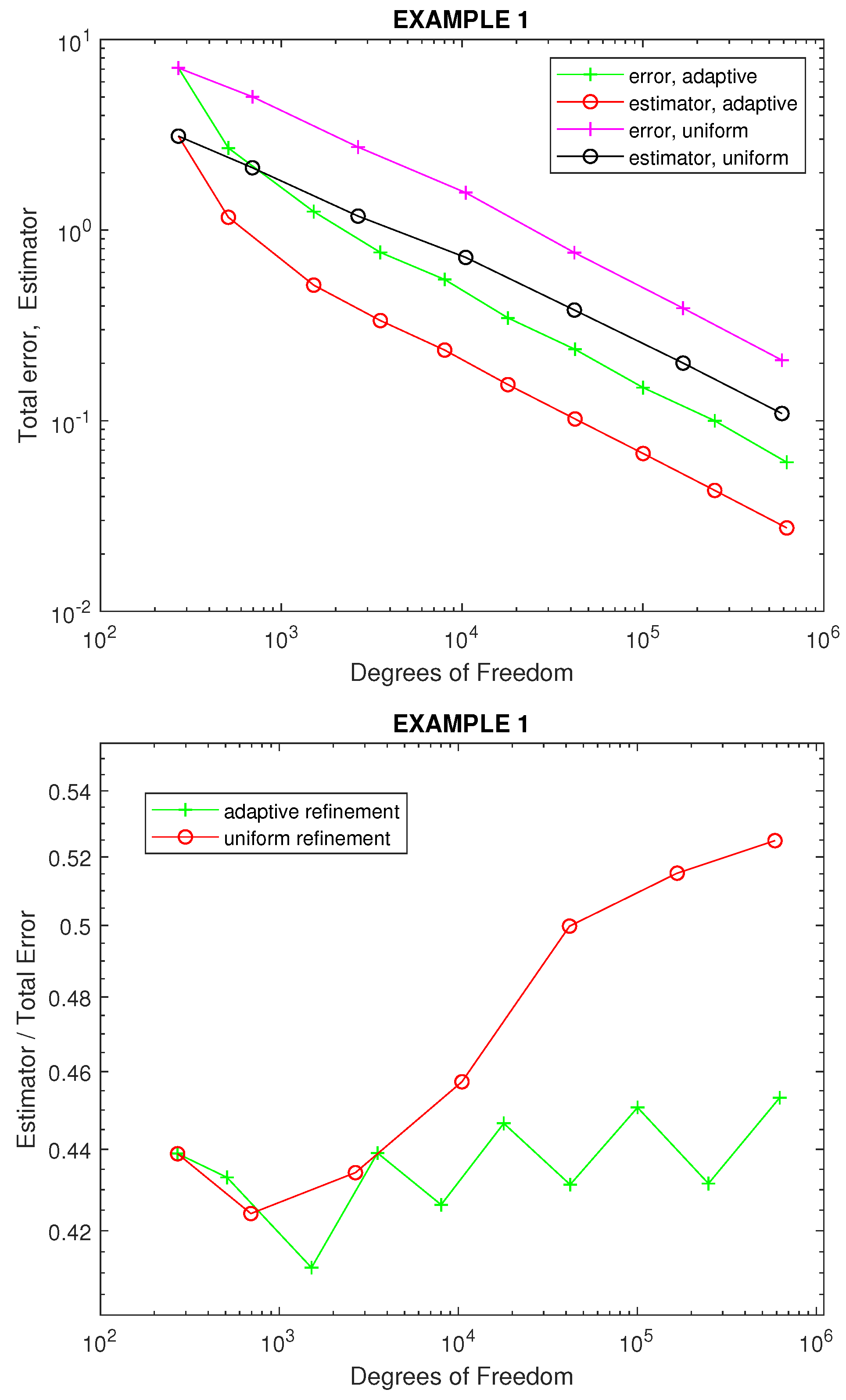
Thus the solution has a singularity in pressure close to the line $x=1$. Figure 2 shows the mesh refinement by the adaptive algorithm. Figure 3, bottom, represents the evolution with respect to degrees of freedom (DOF) of error and indicator; on the right, we can observe the evolution of the efficiency index with DOF.

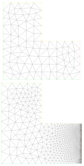
Figure 2. Example 1. Initial mesh (270 DOF) on the (top); intermediate adapted mesh with 1512 DOF on the (bottom).

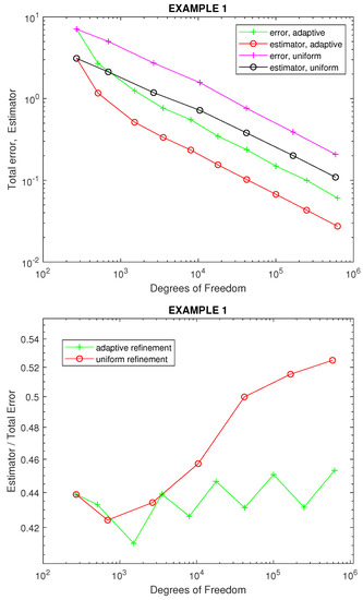
Figure 3. Example 1. (Top): Error and indicator evolution vs. DOF. (Bottom): Efficiency index vs. DOF.

5. Discussion

The adaptive algorithm was tested on an example with a singularity. From Figure 2 we can observe that the algorithm refined the mesh near the singularity, as expected. Since it is an academic example with a known solution, we could compute the exact error. The graphs in Figure 3 confirm that the error was lower for the adaptive refinement. Additionally, since the exact error and estimator followed close to parallel lines, we confirm that the indicator gives a consistent measure of the error. This could also be checked by the efficiency index, which is the ratio of indicator to exact total error.

References

- Girault, V.; Wheeler, M.F. Numerical Discretization of a Darcy-Forchheimer Model. Numer. Math. 2008, 110, 161–198. [Google Scholar] [CrossRef]
- Salas, J.J.; López, H.; Molina, B. An analysis of a mixed finite element method for a Darcy-Forchheimer model. Math. Comput. Model. 2013, 57, 2325–2338. [Google Scholar] [CrossRef]
- Borouchaki, H.; Hecht, F.; Frey, P. Mesh gradation control. Int. J. Numer. Meth. Eng. 1998, 43, 1143–1165. [Google Scholar] [CrossRef]
- Hetch, F. FreeFEM Documentation, Release 4.6. 2020. Available online: https://doc.freefem.org/pdf/FreeFEM-documentation.pdf (accessed on 13 October 2021).
Publisher’s Note: MDPI stays neutral with regard to jurisdictional claims in published maps and institutional affiliations. |
© 2021 by the authors. Licensee MDPI, Basel, Switzerland. This article is an open access article distributed under the terms and conditions of the Creative Commons Attribution (CC BY) license (https://creativecommons.org/licenses/by/4.0/).