Time Series Sampling ^†

Abstract

Some complex models are frequently employed to describe physical and mechanical phenomena. In this setting, we have an input X, which is a time series, and an output $Y=f\left(X\right)$ where f is a very complicated function, whose computational cost for every new input is very high. We are given two sets of observations of X, $S_1$ and $S_2$ of different sizes such that only $f\left(S_1\right)$ is available. We tackle the problem of selecting a subsample $S_3\in S_2$ of a smaller size on which to run the complex model f and such that distribution of $f\left(S_3\right)$ is close to that of $f\left(S_1\right)$. We adapt to this new framework five algorithms introduced in a previous work "Subsampling under Distributional Constraints" to solve this problem and show their efficiency using time series data.

1. Introduction

The study of the damage caused over time and stress on a mechanical part allows for prediction of the failure of this part [1,2]. For this, it is necessary, on the one hand, to have reliable data and, on the other hand, to have a model that is faithful to reality. Such models are used to generate some scenarios using the solution of partial derivative equations (PDEs). Their input is often composed of different variables in the form of a time series denoted by X, and their output $f\left(X\right)$ may be multidimensional and depend on space and time. The use of such models consists of solving complicated PDEs, and each generated scenario corresponds in the machine learning paradigm to an inference for a new input X, and, therefore, to the computation of $f\left(X\right)$. The more complex that these models are, and the closer they are to reality, the more expensive they are in terms of computing time and power. In practice, these calculations can take days or weeks.

Consider a set $S_1=\{X_1,\dots ,X_{n_1}\}$ with a distribution similar to that of the time series X lying in a separable metric space $(\mathcal{E},\rho )$. To each observation, we apply a deterministic smooth function. This function, $f:\mathcal{E}\to \mathbb{R}$, is expensive and complex and may be seen as a black box. Moreover, we have a large sample $S_2$ of size $n_2$ with the same distribution as X. We do not know the values $f\left(S_2\right)$. The goal is to find a subsample $S_3\subset S_2$ of a size $n_3$ smaller than $n_2$ in such a way that the distribution of $f\left(S_3\right)$ is close to that of $f\left(S_1\right)$.

At first sight, this is a classic sampling problem. We can use sampling techniques identical to those used in surveys as well as unsupervised [3] or supervised techniques [4,5,6]. Some recent algorithms were proposed in [7] to solve this problem for the general case of variable X that lies in any metric space. We are interested, in this paper, in adapting such algorithms for the case in which X is a time series. We explore, in this paper, two possible adaptations; the first consists of encoding the time series X by independent features, and the second using appropriate distances between time series and adjusting the sampling algorithms to use such distances.

This manuscript is organized as follows. In Section 2, we fix some notations that will be used throughout the manuscript, and we specify the framework of the problem to be solved. In Section 3, we describe the algorithms used in [7] to solve the problem. In Section 4, we suggest alternative adaptations for these algorithms for their application to time series. Section 5 gives an industrial application of these approaches. In Section 6, some concluding remarks are provided.

2. The Problem Setting

Let $S_1=\{X_1,\dots ,X_{n_1}\}$ as a set of $n_1$ time series following the same distribution $\mu$ as X, and ${\mathcal{S}}_2=\{X_1^{\prime },\dots ,X_{n_2}^{\prime }\}$ as a second set of time series of size $n_2$ coming from the same distribution $\mu$. Let $f:\mathcal{E}\to \mathbb{R}$ as a deterministic function that is very complicated and hard to compute. The unknown distribution of $f\left(X\right)$ will be denoted by F. Moreover, we dispose of

$${\mathcal{Y}}_1=:\{Y_i=f\left(X_i\right)fori=1,\dots n_1\}$$

of the images of the first sample ${\mathcal{S}}_1$ denoted $f\left(S_1\right)$. The images of $S_2$ by f are not available.

From this information, we want to determine a subsample ${\mathcal{S}}_3\subset {\mathcal{S}}_2$ of size $n_3<<n_2$ in such a way that the empirical distribution of $f\left(S_3\right):=\{f\left(X_j\right):X_j\in S_3\}$ will be close to the distribution of $f\left(X_1\right)$.

Several approaches are possible for this problem in a general setting in which X is a random variable in a separable metric space.

If ${\mu }_1$ stands for the empirical distribution of ${\mathcal{S}}_1$ and ${\mu }_3$ for that of a subset ${\mathcal{S}}_3\subset {\mathcal{S}}_2$, and the function f is regular, we look for a subset ${\mathcal{S}}_3$ such that a:

$$d({\mu }_1,{\mu }_3),$$

(1)

is minimal among all possible subsets. Here, d is a distance metrizing weak convergence, similar to the Prokhorov distance. In the next section, we will describe some algorithms proposed in [7] to solve this problem and that we aim to adapt to the time series.

3. Sampling Algorithms

We describe briefly some existing algorithms designed to solve our problem in a general context where X is a random variable that lies in any metric space. A more detailed description of these approaches may be found in [7].

Let $S_1=\{X_1,\cdots X_{n_1}\}$ and $S_2=\{X_1^{\prime },\cdots X_{n_2}^{\prime }\}$ be two independent samples with $n_2>n_1$ that come from the same distribution of X.

Among the following algorithms, some make use of ${\mathcal{Y}}_1$, and others do not.

3.1. Extended Nearest Neighbors Approach

This algorithm does not make use of ${\mathcal{Y}}_1$. The selected subset $S_3$ is simply the set of the nearest extended neighbors of $S_1$ in $S_2$. Consider the nearest neighbors of $S_1$ in $S_2$, $d_1,\cdots ,d_{n_1}$, their ordered distances and $j\left(1\right),\cdots j\left(n_1\right)$ their indices.

Suppose that two elements of $S_1$, called $X_i$ and $X_j$, have identical nearest neighbors, $X_l^{\prime }$, with respective distances $d_i$ and $d_j$, and suppose that if $d_i<d_j$, then $X_l^{\prime }$ will be the nearest neighbor of $X_i$, while for $X_j$ we will have to take its second nearest neighbor, and so on. This approach is based on the idea that if the elements of $S_2$ are close to those of $S_1$, then the images of $S_3$ by f should be close to those of $S_1$.

3.2. A Partition-Based Algorithm

For this algorithm, a partition of the set ${\mathcal{Y}}_1$ into L clusters of size m is built s.t. $n=mL$ Denote the clusters by $C_k$, their complements by $C_{n-k}=S_1\setminus C_k$ and $F_k$ the empirical cdf of Y in $C_k$. Denote by ${\widehat{C}}_k$ the cluster which minimizes $\parallel F_k-F_{n-k}\parallel$, and the subset ${\tilde{C}}_k=\{X_{i1},\dots X_{ik}\}\subset S_1$ fulfilling $f\left({\tilde{C}}_k\right)={\widehat{C}}_k$ which is a subset of $S_1$. $S_3$ is defined as the set of the nearest neighbors of ${\tilde{C}}_k$ from $S2$. The partition used in this algorithm may be any random partition, or any partition obtained from a clustering algorithm similar to k-means.

3.3. A Histogram-Based Approach

The idea in this algorithm is to use the empirical distribution of the sample ${\mathcal{Y}}_1$. First, ${\mathcal{Y}}_3$ is obtained by a stratified sampling from ${\mathcal{Y}}_1$ where the stratas are obtained using the bins of the histogram built on ${\mathcal{Y}}_1$. $S_3$ is then taken to be the set of the nearest neighbors of $f^{-1}\left({\mathcal{Y}}_3\right)$ from $S_2$. The empirical distribution of $f\left(S_3\right)$ is close to that of $f\left(S_1\right)$, $S_1$, and the $S_3$ distributions are expected to be close if f is smooth. Two alternatives to this algorithm have been proposed in [7], replacing the stratified sampling to get ${\mathcal{Y}}_3$ with either the support points approach [3] or the D-optimality [4].

4. Adaptation of Algorithms to Time Series

We suppose that the time series available in both samples $S_1$ and $S_2$ have different lengths. In this section, we will show how the algorithms presented in Section 3 may be adjusted to be used when X is a time series. For this purpose, two approaches are considered, encoding and choosing appropriate distances for time series. For the first approach, each time series in the data is embedded in a vectorial metric space through feature extraction; features may be used arbitrarily or obtained from an autoregressive linear model applied to each time series.

4.1. Encoding

We experiment with two types of encodings.

• Simple statistical feature extraction
  The p statistical characteristics are computed for each time series. These include the minimum, maximum, sum, number of times a threshold is crossed, length of zero periods, and so on. These engineering features depend on the dataset at hand and its characteristics.
• Using linear autoregressive (AR) models
  A linear autoregressive model is adjusted to each time series with a maximum order $pmax$. Once the optimal orders $p_j$ are obtained for all time series in any sample, we fix the final desired order as $p=ma{x}_j\left\{p_j\right\}$. Finally, each time series is represented by its p estimated coefficients.

4.2. Using Appropriate Distance

Most of the algorithms described in Section 3 are based on neighborhood and, thus, distances. Here, we suggest replacing the Euclidean distance used in the general framework with dynamic time warping (DTW).

DTW allows for comparison of two time series by measuring their similarity, even if they have different lengths [8,9].

Consider the two time series $A=\{A_1,\dots ,A_n\}$ and $B=\{B_1,\dots ,B_m\}$ with $n\ne m$, which lie in the same dimensional space. The goal of DTW is to find the optimal temporal alignment between A and B; each point from A is associated with at least one point from B (and reciprocally), as shown in Figure 1. The optimal alignment, corresponding to the DTW distance between A and B, is the one giving the minimum total length between the couples of aligned points. This may be computed by resolving a linear programming problem.

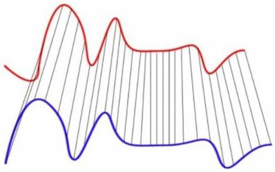
Figure 1. Time points alignment between two time series [10].

For a long time series, the DTW may be very complex to compute. The computation may be simplified using fast versions of the underlying optimization algorithm or by sampling the time series using arbitrary frequencies.

5. Real Dataset Application

We apply now the proposed approach to a time series dataset concerning real customers provided by RENAULT ( the French car industry). All experiments were run using the R software [11] together with packages [12,13].

5.1. Driving Behavior Dataset

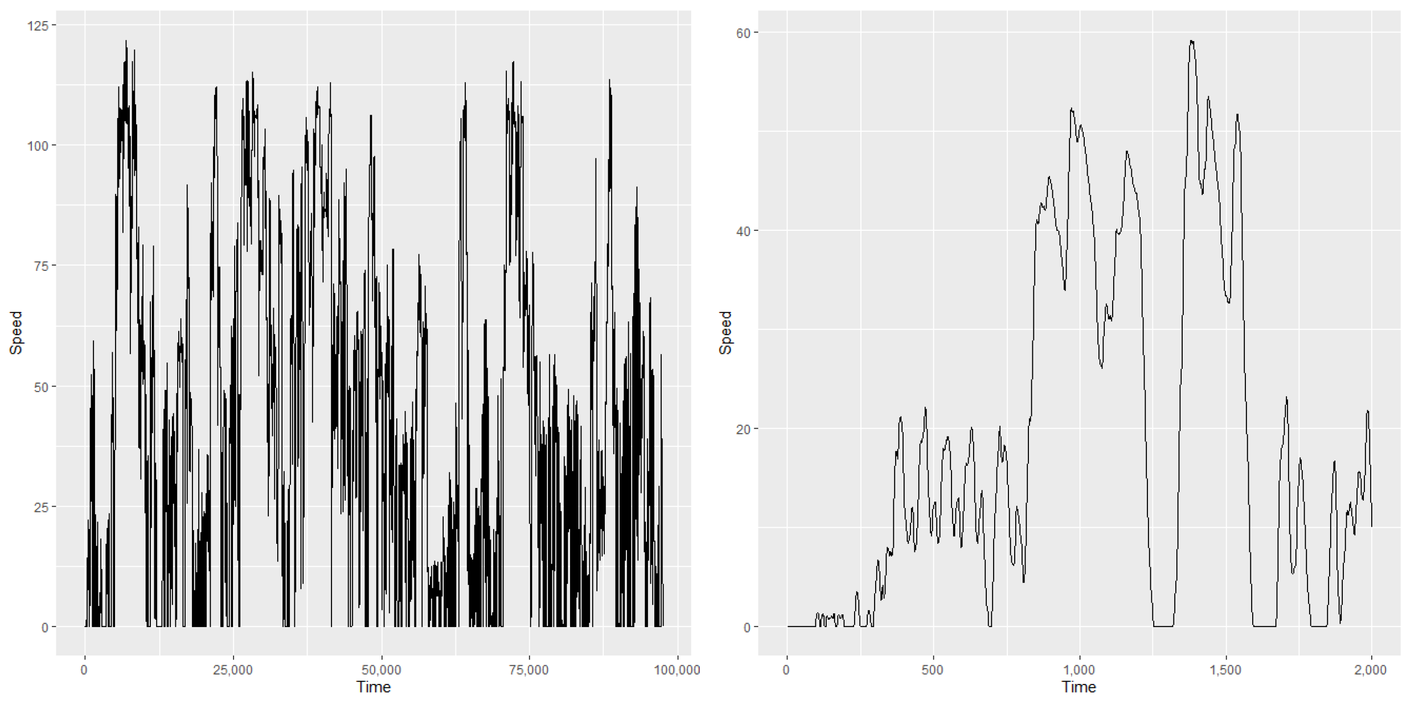
The variable X in our dataset is the time series of driver’s speed. A large number of time series are available sampled at 5 Hz with a recording duration varying from a few days to a few weeks. Sampling at 5 Hz represents 86,400 points per day. This means that the time series studied are very large and different. An example of such time series is provided in Figure 2. We have used a selected sample of 691 customers.

Figure 2. Complete driver’s speed (left) and zoomed part (right).

As these time series are speed traces of real customers, they vary from 0 to 150 km/h in our sample. Long and short stays at zero may be observed in these time series, corresponding to either night periods or shorter periods that correspond to car pauses, such as those for red lights. The lengths of the time series in our sample vary from 25,000 points to several million. Figure 3 shows the distribution of the time series lengths and the distribution of the zero values among the time series.

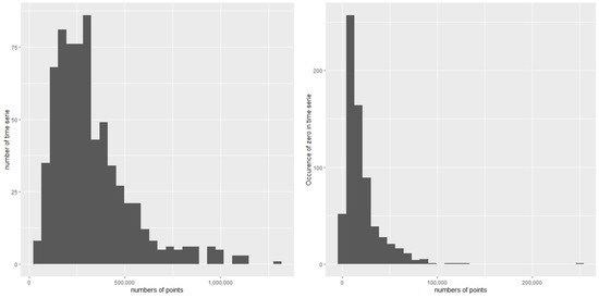
Figure 3. Histograms of time series length (right) and number of zeroes in each time series (left).

In addition, for the 691 customers, a complex numerical model f was run in order to estimate the maximum soot released from each customer’s vehicle. This model requires as input x the speed data time series together with many other characteristics of the vehicle. The maximum soot is the output of interest. As this model requires very long time computations (several hours for each customer depending on its parametrization), the objective is to select from among a dataset not used with the model, such as a sample of customers, for which the model would issue a similar distribution for the maximum soot to that already modeled for the customers.

5.2. Results

In this section, we provide the results of the algorithms proposed in Section 3: the extended nearest neighbors, the partition-based algorithm, the histogram-based approach and both variants using the support point and D-optimality.

To test these algorithms, the sample was randomly split into two parts with $S_1$ having 100 customers, and $S_2$ having the other 591. Each algorithm was run 100 times, and, from each run, the obtained optimal subsample $S_3$ was compared to $S_1$ using the Kolmogorov–Smirnov (KS) two samples test between $f\left(S_1\right)$ and $f\left(S_3\right)$, as the output of the model is known for all the samples in our dataset. Table 1 gives the average values of the KS statistics and the p-values over the 100 runs. We can observe that, depending on the encoding used, the algorithms do not react in the same way. We can see that the histogram-based algorithm provides the same results for the AR coefficients and feature extraction, though it is less efficient with the DTW. For the partition-based algorithms, the DTW performs much better than the two encoding approaches. While for the nearest neighbors and the support point, we get very close results for both encodings. Finally, for the D-optimality, we can see that the DTW and AR features provide the same results, which are better than those for feature extraction.

Table 1. Average results for each encoding and for each algorithm over 100 runs. NN = nearest neighbors.

Encoding	Autoregressive			Feature Extraction			Dynamic Time Warping
Algorithm	${\mathit{N}}_3$	Stat	p-Value	${\mathit{N}}_3$	Stat	p-Value	${\mathit{N}}_3$	Stat	p-Value
Extended NN	88	$0.12$	$0.53$	91	$0.11$	$0.60$	100	$0.11$	$0.59$
Partition-based	10	$0.27$	$0.57$	10	$0.27$	$0.55$	69	$0.13$	$0.53$
Histogram-based	48	$0.44$	$0.0001$	48	$0.44$	$0.0001$	48	$0.46$	$0.0001$
D-optimality	100	$0.12$	$0.54$	16	$0.21$	$0.61$	100	$0.11$	$0.59$
Support point	50	$0.15$	$0.50$	50	$0.14$	$0.59$	50	$0.14$	$0.57$

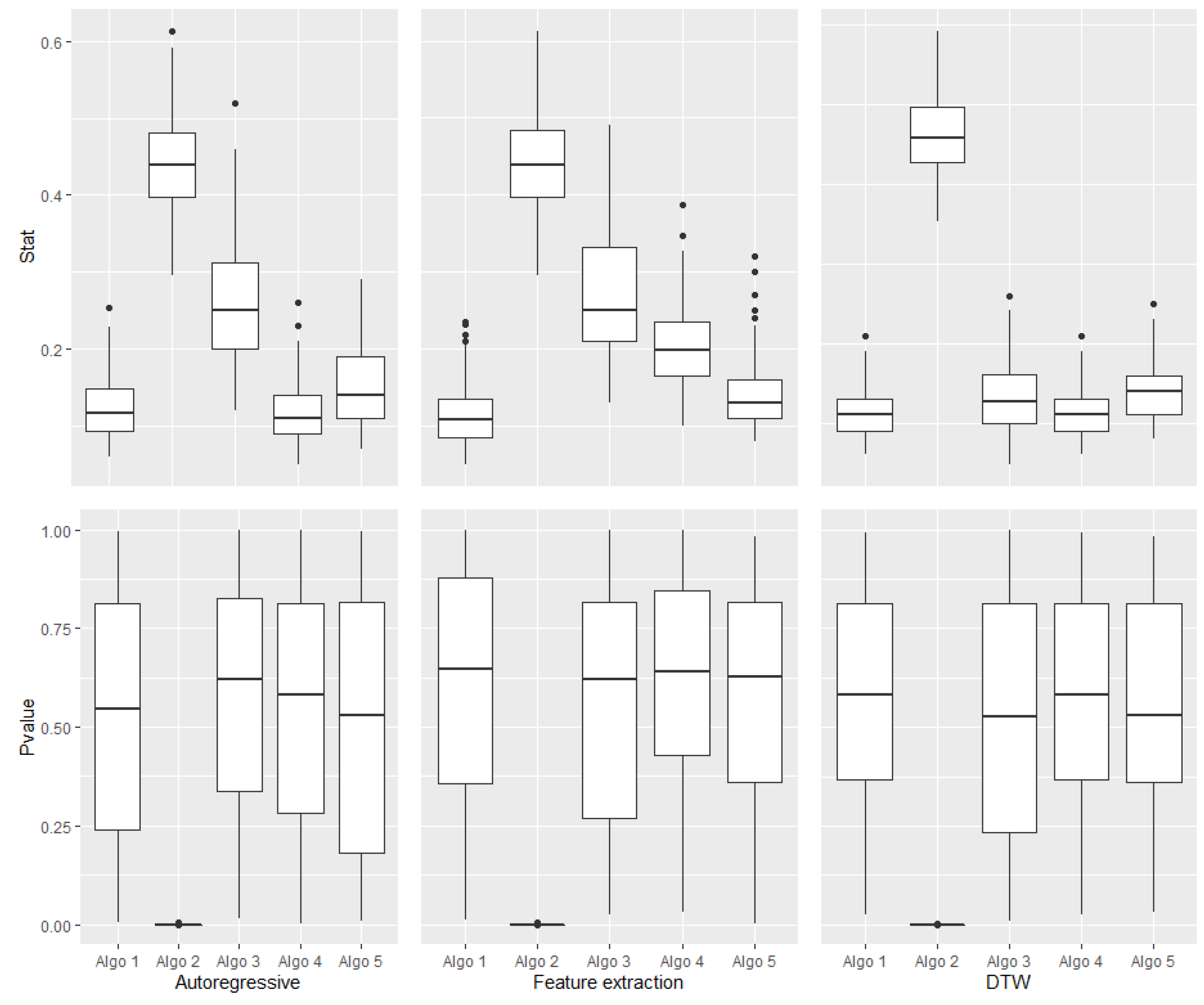
Figure 4 shows the distribution of the p-values and the KS statistics over the 100 runs for all algorithms, the two encodings and DTW.

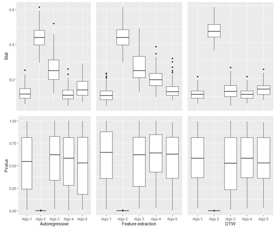
Figure 4. Results of all algorithms by encoding from left to right: AR features, feature extraction and DTW. Algo 1 = Extended nearest neighbors; Algo 2 = Histogram-based; Algo 3 = Partition-based; Algo 4 = D-optimality; Algo 5 = Support point.

We can see that the deviation of the computed statistics are different for the three approaches: the AR, feature extraction and DTW. We can see that, for all algorithms, the AR encoding results are more unstable than those of the two other approaches.

6. Discussion and Conclusions

In this work, we have tackled the problem of selecting a subsample of time series to satisfy some distributional constraints. We have adapted several algorithms proposed recently in a more general framework to our context. All of the proposed approaches were tested over a real dataset of a car’s speed time series. The results obtained show that our algorithms work as expected, except for one approach: the histogram-based one. To adapt the existing algorithms we have suggested various numerical representations for the time series and shown that different choices for encoding may affect the results significantly. More complex models than the autoregressive approach, or more refined statistical representations for the time series, might be more efficient. One idea under investigation is to use supervised embedding through recurrent neural networks.

References

- García Márquez, F.P.; Pedregal, D.; Roberts, C. Time series methods applied to failure prediction and detection. Reliab. Eng. Syst. Saf. 2010, 95, 698–703. [Google Scholar] [CrossRef]
- Khatkhate, A.; Ray, A.; Keller, E.; Gupta, S. Symbolic Time Series Analysis of Mechanical Systems for Anomaly Detection. ASME/IEEE Trans. Mechatron. 2006, 11, 439–447. [Google Scholar] [CrossRef]
- Joseph, V.R.; Mak, S. Support points. Ann. Stat. 2018, 46, 2562–2592. [Google Scholar] [CrossRef]
- Wang, H.Y.; Min, Y.; John, S. Information-Based Optimal Subdata Selection for Big Data Linear Regression. J. Am. Stat. Assoc. 2019, 114, 393–405. [Google Scholar] [CrossRef]
- Wang, H.Y.; Rong, Z.; Ping, M. Optimal Subsampling for Large Sample Logistic Regression. J. Am. Stat. Assoc. 2018, 113, 829–844. [Google Scholar] [CrossRef] [PubMed]
- Joseph, V.R.; Mak, S. Supervised compression of big data. Stat. Anal. Data Min. Asa Data Sci. J. 2021, 14, 217–229. [Google Scholar] [CrossRef]
- Combes, F.; Fraiman, R.; Ghattas, B. Subsampling under Distributional Constraints; Working Paper. Available online: https://hal.archives-ouvertes.fr/hal-03666898/file/OptimalSampling.pdf (accessed on 15 April 2022).
- Sakoe, H.; Chiba, S. Dynamic programming algorithm optimization for spoken word recognition. IEEE Trans. Acoust. Speech Signal Process. 1978, 26, 43–49. [Google Scholar] [CrossRef]
- Vintsyuk, T.K. Speech discrimination by dynamic programming. Cybernetics 1968, 4, 52–57. [Google Scholar] [CrossRef]
- Martin, D.; Serrano, A.; Bergman, A.W.; Wetzstein, G.; Masia, B. ScanGAN360: A Generative Model of Realistic Scanpaths for 360° Images. arxiv 2013, arXiv:2103.13922. [Google Scholar] [CrossRef] [PubMed]
- R Core Team. R: A Language and Environment for Statistical Computing; R Foundation for Statistical Computing: Vienna, Austria, 2022. [Google Scholar]
- Mak, S. Support: Support Points, R Package Version 0.1.5; 2021. Available online: https://CRAN.R-project.org/package=support (accessed on 15 April 2022).
- Giorgino, T. Computing and Visualizing Dynamic Time Warping Alignments in R: The dtw Package. J. Stat. Softw. 2009, 31, 1–24. [Google Scholar] [CrossRef]
Publisher’s Note: MDPI stays neutral with regard to jurisdictional claims in published maps and institutional affiliations. |
© 2022 by the authors. Licensee MDPI, Basel, Switzerland. This article is an open access article distributed under the terms and conditions of the Creative Commons Attribution (CC BY) license (https://creativecommons.org/licenses/by/4.0/).