Modelling a Continuous Time Series with FOU(p) Processes ^†

Abstract

In this work we summarize the knowledge about FOU(p) processes (fractional iterated Ornstein–Uhlenbeck processes of order emphp). Fractional Ornstein–Uhlenbeck processes are a particular case of FOU(p) processes (when $p=1$). FOU(p) processes are able to model time series with both long- and short-range dependence. We give the definition, the main theoretical properties, and a procedure for estimating the parameters consistently. We also show how to model a continuous time series with FOU(p) processes, and we give an example of an application.

1. Introduction

Usually, in time series, the researcher has a series of measurements evenly spaced in time (for example, measurements per minute, every thirty seconds, or weekly measurements). In these cases the underlying process is continuous time. The fractional iterated Ornstein–Uhlenbeck processes of order p (that we call FOU$\left(p\right)$ and which are defined in [1]) are stationary and centred Gaussian continuous-time processes. By construction, the FOU$\left(p\right)$ process depends on the two parameters defining the underlying fractional Brownian motion, namely, the Hurst exponent (H) and the scale parameter $\sigma$. From the relationship between the variogram and the Hölder index of the process trajectories, using a result given in [2], it is proved in [1] that H is the Hölder index of a FOU$\left(p\right)$, giving information about the irregularity of the trajectories. If the process is observed in a discretized and equispaced interval $[0,T]$, by applying a procedure suggested in [3] it is possible to estimate H and $\sigma$ consistently. Apart from H and $\sigma$, a FOU$\left(p\right)$ process is determined by a set of additional parameters, the so-called $\lambda$ parameters, giving information about the local dependence. The theoretical properties of any FOU$\left(p\right)$ process and a methodology for estimating its parameters consistently (including the asymptotic behaviour) are given in [1]. The estimation method and the asymptotic results for the $\lambda$ parameters were obtained under the assumption that the process is observed over the entire interval $[0,T]$, where $T\to \infty$. In [4], a consistent method can be found for estimating the $\lambda$ parameters in the discretized case. An interesting property of the FOU$\left(p\right)$ process is that it exhibits short-range dependence when $p\ge 2$, even though $H>1/2$ (in this case, the generating fractional Brownian motion has long-range dependence). In addition, when $p=1$ we have the result that FOU$\left(1\right)$ is the classical fractional Ornstein–Uhlenbeck process (fOU) defined in [5], which has long-range dependence when $H>1/2$. Another interesting property is that as p grows, the autocorrelation function of the process goes more quickly to zero. In addition, FOU$\left(1\right)$ (fOU) processes can be approximated by FOU$\left(2\right)$ (simply taking ${\lambda }_1\to 0$, where $\lambda =({\lambda }_1,{\lambda }_2)$). Thus, FOU$\left(p\right)$ processes can be viewed as a generalization of fOU processes and are able to model a time series with short-range dependence or long-range dependence. The main objective of this work is to summarize the results obtained in [1,4,6] for modeling a time series through FOU$\left(p\right)$ processes. In Section 2, we give the definition of a FOU$\left(p\right)$ process. The method for estimating its parameters is given in Section 3. In Section 4, we give a method of modeling a time series through the FOU$\left(p\right)$ process, including an example. Some conclusions are given in Section 5.

2. Definition of FOU(p) Processes

FOU$\left(p\right)$ processes are built from the fractional Brownian motion.

Definition 1.

A fractional Brownian motion with Hurst parameter $H\in \left(0,1\right]$ is an almost surely continuous centred Gaussian process ${\left\{B_H\left(t\right)\right\}}_{t\in \mathbb{R}}$ such that its auto-covariance function is

$$\mathbb{E}\left(B_H\left(t\right)B_H\left(s\right)\right)=\frac{1}{2}\left({\left|t\right|}^{2H}+{\left|s\right|}^{2H}-{\left|t-s\right|}^{2H}\right)foreveryt,s\in \mathbb{R}.$$

To use a fractional Brownian motion with a scale parameter $\sigma$, we use the notation ${\left\{\sigma B_H\left(t\right)\right\}}_{t\in \mathbb{R}}$.

Now, we can define a fractional iterated Ornstein–Uhlenbeck process of order p (FOU$\left(p\right)$), as found in [1].

Definition 2.

Let ${\left\{\sigma B_H\left(s\right)\right\}}_{s\in \mathbb{R}}$ be a fractional Brownian motion with Hurst parameter H and scale parameter σ. Suppose further that ${\lambda }_1,{\lambda }_2,\cdots ,{\lambda }_q$ are pairwise different and positive numbers and $p_1,p_2,\cdots ,p_q\in \mathbb{N}$ such that $p_1+p_2+\cdots +p_q=p$. Then, the fractional iterated Ornstein–Uhlenbeck process of order p is defined as

$$X_t:=T_{{\lambda }_1}^{p_1}\circ T_{{\lambda }_2}^{p_2}\circ ....\circ T_{{\lambda }_q}^{p_q}\left(\sigma B_H\right)\left(t\right)=\sum _{i=1}^q{K}_i\left(\lambda \right)\sum _{j=0}^{p_i-1}\left(\genfrac{}{}{0pt}{}{p_i-1}{j}\right)T_{{\lambda }_i}^{\left(j\right)}\left(\sigma B_H\right)\left(t\right),$$

where the numbers $K_i\left(\lambda \right)$ are defined by

$$K_i\left(\lambda \right)=K_i\left({\lambda }_1,{\lambda }_2,\cdots ,{\lambda }_q\right):=\frac{1}{{\displaystyle \prod _{j\ne i}}\left(1-{\lambda }_j/{\lambda }_i\right)}$$

(1)

and the operators $T_{{\lambda }_i}^{\left(j\right)}$ are defined by

$$T_{\lambda }^{\left(h\right)}\left(y\right)\left(t\right):={\int }_{-\infty }^t{e}^{-\lambda (t-s)}\frac{{\left(-\lambda \left(t-s\right)\right)}^h}{h!}dy\left(s\right)forh=0,1,2,\cdots$$

(2)

We define $T_{\lambda }$ simply for the $h=0$ case, that is

$$T_{\lambda }\left(y\right)\left(t\right):={\int }_{-\infty }^t{e}^{-\lambda (t-s)}dy\left(s\right).$$

(3)

Remark 1.

The equality $T_{{\lambda }_1}^{p_1}\circ T_{{\lambda }_2}^{p_2}\circ ....\circ T_{{\lambda }_q}^{p_q}={\sum }_{i=1}^q{K}_i\left(\lambda \right){\sum }_{j=0}^{p_i-1}\left(\genfrac{}{}{0pt}{}{p_i-1}{j}\right)T_{{\lambda }_i}^{\left(j\right)}$ that appears in Definition 2 is proved in [7].

Remark 2.

The equality $T_{{\lambda }_1}^{p_1}\circ T_{{\lambda }_2}^{p_2}\circ ....\circ T_{{\lambda }_q}^{p_q}={\sum }_{i=1}^q{K}_i\left(\lambda \right){\sum }_{j=0}^{p_i-1}\left(\genfrac{}{}{0pt}{}{p_i-1}{j}\right)T_{{\lambda }_i}^{\left(j\right)}$ implies that the composition $T_{{\lambda }_1}^{p_1}\circ T_{{\lambda }_2}^{p_2}\circ ....\circ T_{{\lambda }_q}^{p_q}$ is commutative. Then, we assume that ${\lambda }_1<{\lambda }_2<\cdots <{\lambda }_q$. This will be helpful for estimating $\lambda =({\lambda }_1,{\lambda }_2,\cdots ,{\lambda }_q)$, to avoid ambiguity.

Notation 1.

${\left\{X_t\right\}}_{t\in \mathbb{R}}\sim \mathrm{FOU}\left({\lambda }_1^{\left(p_1\right)},{\lambda }_2^{\left(p_2\right)},\cdots ,{\lambda }_q^{\left(p_q\right)},\sigma ,H\right),$ where $0<{\lambda }_1<{\lambda }_2<\cdots <{\lambda }_q$, or more simply, ${\left\{X_t\right\}}_{t\in \mathbb{R}}\sim$FOU$\left(p\right)$.

Remark 3.

The notation FOU$\left({\lambda }_1^{\left(p_1\right)},{\lambda }_2^{\left(p_2\right)},\cdots ,{\lambda }_q^{\left(p_q\right)},\sigma ,H\right)$ implies that $0<{\lambda }_1<{\lambda }_2<\cdots <{\lambda }_q$. On the other hand, the notation FOU$\left(p\right)$ means that we have taken p times the composition of operators $T_{\lambda }$ for different or equal values of λ.

Remark 4.

Every FOU$\left({\lambda }_1^{\left(p_1\right)},{\lambda }_2^{\left(p_2\right)},\cdots ,{\lambda }_q^{\left(p_q\right)},\sigma ,H\right)$ is a Gaussian, centred, almost surely continuous process and is almost surely non-differentiable at any point (the proof of these results can be found in [1]).

Remark 5.

When $p=1$, FOU$\left(\lambda ,\sigma ,H\right)$ is the classical fractional Ornstein–Uhlenbeck process.

Remark 6.

In the case in which $p_1=p_2=\cdots =p_q=1$, we have

$$X_t=T_{{\lambda }_1}\circ T_{{\lambda }_2}\circ \cdots \circ T_{{\lambda }_q}\left(\sigma B_H\right)\left(t\right)=\sum _{i=1}^q{K}_i\left(\lambda \right)T_{{\lambda }_i}\left(\sigma B_H\right)\left(t\right)$$

(4)

and we simply write ${\left\{X_t\right\}}_{t\in \mathbb{R}}\sim$FOU$\left({\lambda }_1,{\lambda }_2,\cdots ,{\lambda }_q,\sigma ,H\right).$

Remark 7.

From Equation (4) we have that any FOU$({\lambda }_1,{\lambda }_2,\sigma ,H)$ where $0<{\lambda }_1<{\lambda }_2$ can be writing as

$$X_t=\frac{{\lambda }_1}{{\lambda }_1-{\lambda }_2}{X}_t^{\left(1\right)}+\frac{{\lambda }_2}{{\lambda }_2-{\lambda }_1}{X}_t^{\left(2\right)}$$

(5)

being $X_t^{\left(i\right)}=\sigma {\int }_{-\infty }^t{e}^{-{\lambda }_i(t-s)}d{B}_H\left(s\right)$ for $i=1,2$. That is, $X_t^{\left(i\right)}$ is a classical fractional Ornstein–Uhlenbeck process with $\lambda ={\lambda }_i.$ Then a FOU$\left(2\right)$ process is a linear combination of two fOU processes with different values of λ.

Remark 8.

From Equation (5), if ${\lambda }_1\to 0$, we have that $X_t\to X_t^{\left(2\right)}$, that is, every fractional Ornstein–Uhlenbeck processes can be approximated by a FOU$\left(2\right)$ process (by taking ${\lambda }_1$ small).

Remark 9.

In [1] it is shown that every FOU$\left(p\right)$ process has a short-range dependence for $p\ge 2$ and every $H\in (0,1)$. On the other hand, it is well-known that if $H>1/2$, every classical Ornstein–Uhlenbeck process has long-range dependence. Therefore, if $H>1/2$, according with previous remark, we have that the short-range dependence FOU$\left(2\right)$ processes can able to approximate a long-range dependence fOU process.

Remark 10.

From remarks 5 and 9, we can say that the FOU$\left(p\right)$ processes are a generalization of fOU processes and are able to model a time series with short-range dependence or long-range dependence.

3. Parameter Estimation

In this section, we summarize a procedure that allows the estimation of the parameters of any FOU$\left(p\right)$ in a consistent way. Similarly to the estimators for $(\lambda ,\sigma ,H)$ proposed in [8] for the fractional Ornstein–Uhlenbeck process, the procedure for estimating the parameters in any FOU$\left(p\right)$ process has two steps. As a first step, we estimate $\sigma$ and H independently of the values of the $\lambda$ parameters. As a second step, using the explicit formula for the spectral density (see Equation (8)) and substituting $(\widehat{H},\widehat{\sigma })$ instead of $(H,\sigma )$, we can estimate $\lambda =\left({\lambda }_1,{\lambda }_2,\cdots ,{\lambda }_q\right)$ using Whittle estimators.

Throughout this section, we assume that we have an equispaced sample in $[0,T]$ of a FOU$\left(p\right)$ process, that is, $X_{T/n},X_{2T/n},....,X_T$, which we simply call $X_1,X_2,\cdots ,X_n$.

3.1. Estimation of H and $\sigma$

We start by recalling the definition of a filter of length $k+1$ and order L.

Definition 3.

$a=\left(a_0,a_1,\cdots ,a_k\right)$ is a filter of length $k+1$ and order $L\ge 1$ when the following conditions are fulfilled:

• ${\sum }_{i=0}^k{a}_i{i}^l=0$ for all $0\le l\le L-1.$
• ${\sum }_{i=0}^k{a}_i{i}^L\ne 0.$

Remark 11.

Given $a,$ a filter of order L and length $k+1$, the new filter $a^2$ defined by $a^2=\left(a_0,0,a_1,0,a_2,0,\cdots ,0,a_k\right)$ has order L and length $2k+1$.

Given a filter a, we can define the quadratic variation of a sample associated with a.

Definition 4.

Given a filter a of length $k+1$ and a sample $X_1,X_2,\cdots ,X_n$, we define

$$V_{n,a}:=\frac{1}{n}\sum _{i=0}^{n-k}{\left(\sum _{j=0}^k{a}_j{X}_{i+j}\right)}^2.$$

If we use a filter a of order $L\ge 2$ and length $k+1$, and we take ${\Delta }_n=n^{-\alpha }$ for some $\alpha >0$ such that $T=n{\Delta }_n\to +\infty$, then if $H>1/2$, the estimators of H and $\sigma$ are given by

$$\widehat{H}=\frac{1}{2}{log}_2\left(\frac{V_{n,a^2}}{V_{n,a}}\right),$$

(6)

$$\widehat{\sigma }={\left(\frac{-2V_{n,a}}{{\Delta }_n^{2\widehat{H}}{\sum }_{i=0}^k{\sum }_{j=0}^k{a}_i{a}_j{\left|i-j\right|}^{2\widehat{H}}}\right)}^{1/2}.$$

(7)

In [1,4], the theoretical details for the asymptotic normality and consistency of $\widehat{H}$ and $\widehat{\sigma }$ can be found.

3.2. Estimation of the $\lambda$ Parameters

If $X={\left\{X_t\right\}}_{t\in \mathbb{R}}\sim$ $FOU({\lambda }_1^{\left(p_1\right)},\dots ,{\lambda }_q^{\left(p_q\right)},\sigma ,H)$, where ${\sum }_{i=1}^q{p}_i=p,$ the spectral density of X is given by (see [1])

$$f^{\left(X\right)}(x,\lambda ,\sigma ,H)=\frac{{\sigma }^2\Gamma (2H+1)sin\left(H\pi \right){\left|x\right|}^{2p-1-2H}}{2\pi {\prod }_{i=1}^q{({\lambda }_i^2+x^2)}^{p_i}}.$$

(8)

From (8), we can estimate $\lambda =\left({\lambda }_1,{\lambda }_2,\cdots ,{\lambda }_q\right)$ using a modified Whittle contrast.

Consider (for any fixed $T>0$) the function

$$\begin{array}{ccc}\hfill U_T^{\left(n\right)}\left(\lambda ,\sigma ,H\right)& =& \frac{T}{n}\sum _{i=1}^n{h}_T^{\left(n\right)}\left(iT/n,\lambda ,\sigma ,H\right)\hfill \end{array}$$

where $h_T^{\left(n\right)}$ is defined by

$$h_T^{\left(n\right)}(x,\lambda ,\sigma ,H)=\frac{1}{2\pi }\left(log{f}^{\left(X\right)}\left(x,\lambda ,\sigma ,H\right)+\frac{I_T^{\left(n\right)}\left(x\right)}{f^{\left(X\right)}\left(x,\lambda ,\sigma ,H\right)}\right)w\left(x\right)$$

where

$$I_T^{\left(n\right)}\left(x\right)=\frac{T}{2\pi }{\left|\frac{1}{n}\sum _{j=1}^n{e}^{\frac{ijTx}{n}}{X}_{\frac{jT}{n}}\right|}^2$$

is the discretization of the periodogram of the process and w is some weight function.

Then, the vector $\lambda$ can be estimated by

$$\begin{array}{ccc}\hfill {\widehat{\lambda }}_T^{\left(n\right)}& =& arg\underset{\lambda \in \mathsf{\Lambda }}{min}{U}_T^{\left(n\right)}\left(\lambda ,\widehat{\sigma },\widehat{H}\right)\hfill \end{array}$$

(9)

where $\widehat{\sigma }$ and $\widehat{H}$ are defined by (7) and (6), respectively, and $\mathsf{\Lambda }$ is some compact set. Details about the consistency of this estimator, including how to choose the w function, can be found in [4].

Remark 12.

When $q=1$, that is, ${\left\{X_t\right\}}_{t\in \mathbb{R}}\sim FOU\left({\lambda }^{\left(p\right)},\sigma ,H\right)$, the λ parameter can be estimated more easily by the following formula:

$$\widehat{\lambda }={\left(\frac{n{\widehat{\sigma }}^2\widehat{H}\Gamma \left(2\widehat{H}\right){\prod }_{i=1}^{p-1}\left(i-\widehat{H}\right)}{\left(p-1\right)!{\sum }_{i=1}^n{X}_i^2}\right)}^{\frac{1}{2\widehat{H}}}.$$

(10)

Theorems on the consistency and asymptotic normality of $\widehat{\lambda }$ can be found in [6].

4. Modelling an Observed Time Series Using FOU$\left(\mathit{p}\right)$ Processes

Of course, before starting to model with FOU$\left(p\right)$ it is necessary to subtract the mean value and remove the seasonal component if it has one. Given $X_1,X_2,\cdots ,X_n$ observations of a stationary centred time series that we wish to model using a FOU$\left(p\right)$ process, we firstly assume that the observations form an equispaced sample on $[0,T]$, that is, $X_{T/n},X_{2T/n},\cdots ,X_T$ for some value of T. According to what was seen in the previous section, we need to estimate $(\lambda ,\sigma$, H), whose estimators depend on T. Thus, firstly we need to know the value of T.

4.1. Choosing the Value of T

To give the value of T is equivalent to give the unit of measurement of time in which the observations are taken. In general, it is natural to take some value of T (for example, if the observations are weekly and we have 104 observations, it is natural to take $T=104$ weeks or $T=2$ years), but we can take any value of T and interpret it (in terms of the original time measure of the data). Therefore, we can choose a value of T that optimizes a certain criterion. According to theoretical results (see [1,4,6]), in order to model a time series dataset using FOU$\left(p\right)$ processes, it is necessary to have values of n and T such that $n,T\to +\infty$ and $T/n\to 0$ at a certain rate. Now, n is the sample size, and the observations lie in the range of $[0,T]$ for some value of T. In [4], it is suggested that a certain value of T should be chosen to optimize some criterion, for example, MAE, RMSE, AIC, BIC, or the Willmott index.

4.2. An Application to Real Data

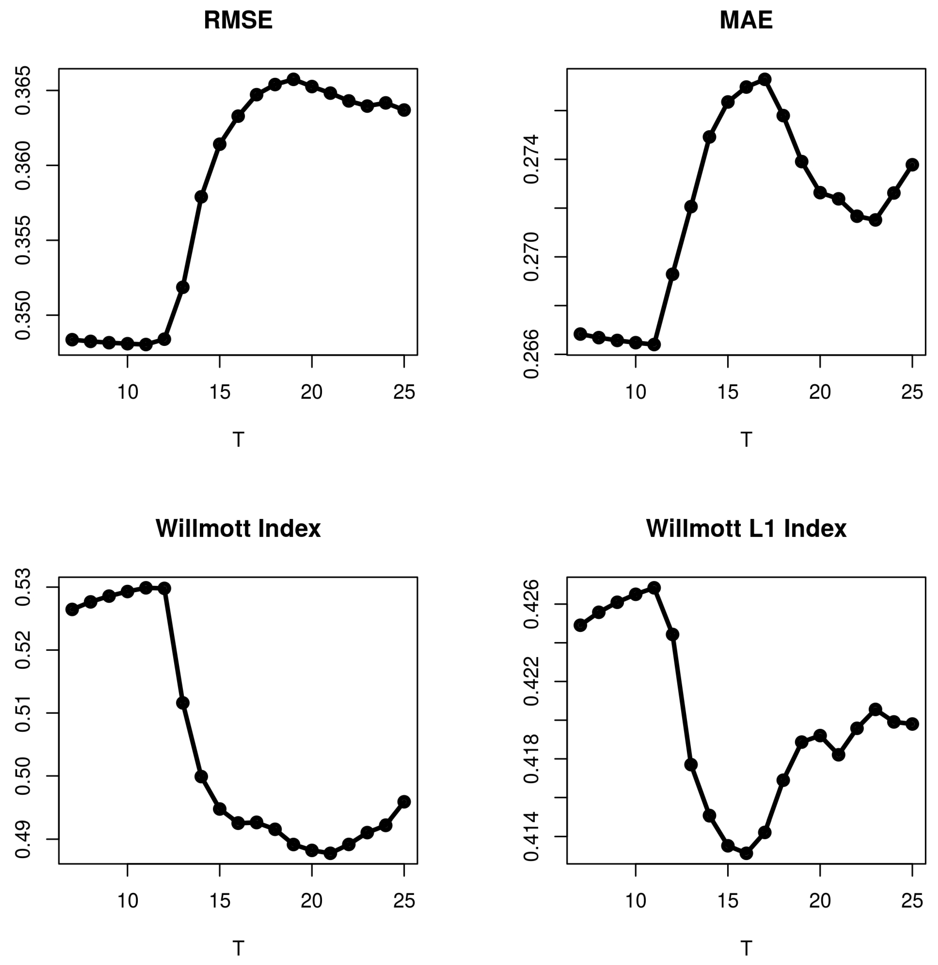
In this section, we work with the well-known Series A (a record of 197 chemical process concentration readings, taken every two hours). To model this with a FOU$\left(p\right)$ process, we use values of $p=2,3,4$. As a first step, for each one of these models, we select a suitable value of T. We minimize the error forecasts for the last m observations

$$\sqrt[h]{\frac{1}{m}\sum _{i=1}^m{\left|X_{n-m+i}-{\widehat{X}}_{n-m+i}\right|}^h}$$

for $h=1$ (mean absolute error, MAE) and $h=2$ (the root mean square error prediction, RMSE) and maximize the Willmott index defined by

$$W_h=1-\frac{{\sum }_{i=1}^m{\left|X_{n-m+i}-{\widehat{X}}_{n-m+i}\right|}^h}{{\sum }_{i=1}^m{\left(\left|{\widehat{X}}_{n-m+i}-\overline{X}\left(m\right)\right|+\left|X_{n-m+i}-\overline{X}\left(m\right)\right|\right)}^h}$$

where $\overline{X}\left(m\right):=\frac{1}{m}{\sum }_{i=1}^m{X}_{n-m+i}$ and $X_1,X_2,\cdots ,X_n$$\left(\mathrm{or}{X}_{T/n},X_{2T/n},\cdots ,X_T\right)$ are the real observations, for $h=1$ and $h=2$. Observe that $W_h$ takes values between 0 and 1, and the predictions improve as $W_h$ grows ($W_2$ is called Willmott index and $W_1$ is called the Willmott $L^1$ index). In

Table 1. Values of W₂, W₁, RMSE, and MAE for different models adjusted to Series A. In bold the optimum value.

Model	${\mathit{W}}_2$	${\mathit{W}}_1$	RMSE	MAE
AR(7)	0.6184	0.4943	0.2995	0.2167
ARMA(1, 1)	0.5883	0.4620	0.3120	0.2343
FOU$\left({\lambda }_1,{\lambda }_2,\sigma ,H\right)$	0.6263	0.4743	0.3076	0.2372
FOU$\left({\lambda }_1,{\lambda }_2,{\lambda }_3,\sigma ,H\right)$	0.6260	0.4743	0.3076	0.2371
FOU$\left({\lambda }_1,{\lambda }_2,{\lambda }_3,{\lambda }_4,\sigma ,H\right)$	0.6244	0.4733	0.3074	0.2369
FOU$\left({\lambda }^{\left(2\right)},\sigma ,H\right)$	0.6247	0.4712	0.3086	0.2393
FOU$\left({\lambda }^{\left(3\right)},\sigma ,H\right)$	0.6277	0.4750	0.3078	0.2373
FOU$\left({\lambda }^{\left(4\right)},\sigma ,H\right)$	0.6264	0.4742	0.3076	0.2372

, we show the values of the four forecast quality measures for the AR$\left(7\right)$, ARMA$(1,1)$ models and every adjusted FOU$\left(p\right)$ models for $p=2,3,4$. Every considered FOU$\left(p\right)$ model, performs similarly and near to AR$\left(7\right)$ in the four measures. In Figure 1, we show the values of the four forecast quality measures in the function of T for the FOU$({\lambda }^{\left(2\right)},\sigma ,H)$ model (the other FOU$\left(p\right)$ models behave similarly) for $m=50$ predictions. That is, for every value of T and every model, we estimate the parameters of the FOU$\left(p\right)$ model and then we obtain the m predictions for the last m observations (at one step) and compute the RMSE, MAE, $W_1$, and $W_2$. In every case, the optimal value is reached in the neighbourhood of $T=11$. To estimate $(\sigma ,H)$, we used a Daubechies filter of order 2:

$$a=\frac{1}{\sqrt{2}}(0.482962,-0.836516,0.224143,0.129409).$$

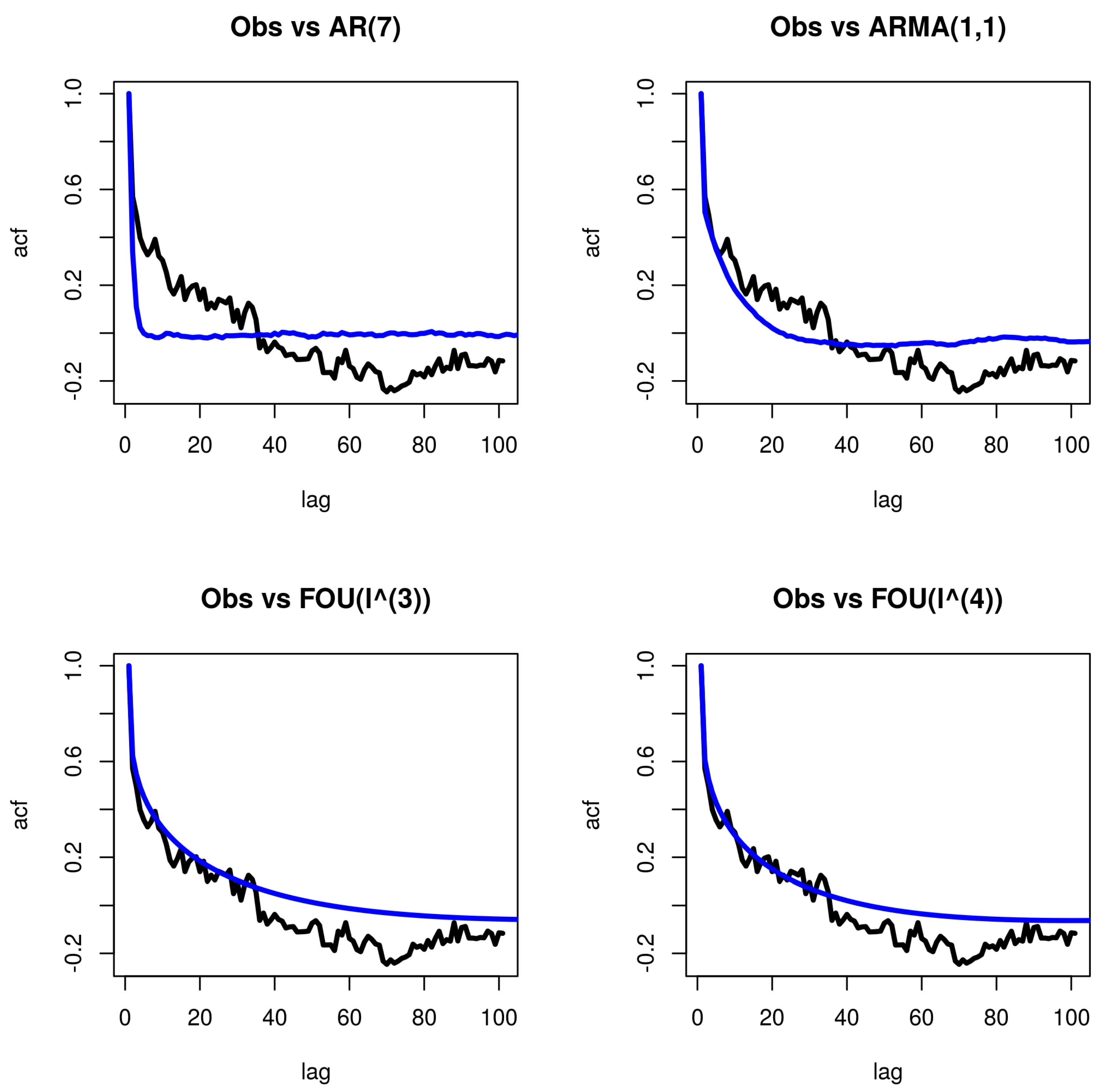
ARMA $(1,1)$ and AR$\left(7\right)$ are suggested for modeling the Series A dataset (see [9] where this dataset was introduced) [10,11]. In Figure 2, we show that the adjusted FOU$({\lambda }^{\left(3\right)},\sigma ,H)$ and FOU$({\lambda }^{\left(4\right)},\sigma ,H)$ have a better fit than the two ARMA models considered.

5. Some Concluding Remarks

We summarize below the main conclusions obtained (details can be found in [1,4,6]):

1.

FOU$\left(p\right)$ processes are a Gaussian family of continuous-time stochastic processes that generalize (by taking $p=1$) the classical fractional Ornstein–Uhlenbeck processes.

2.

When $p\ge 2$, any FOU$\left(p\right)$ has short-range dependence for every value of H, whereas for $p=1$ and $H>1/2$, it is well known that the classical fractional Ornstein–Uhlenbeck process has a long-range dependence. In addition, any long-range dependence fractional Ornstein–Uhlenbeck process ($H>1/2$) can be approximate for some FOU$\left(2\right)$ (short-range dependence).

3.

As p grows, the FOU$\left(p\right)$ process has a shorter memory (in the sense that the autocorrelation function goes more quickly to zero).

4.

Under general conditions, it is possible to estimate all the parameters of any FOU$\left(p\right)$ process in a consistent way.

5.

FOU$\left(p\right)$ processes are able to model a wide range of time series. In [4,6], four examples of real datasets with small and large sample sizes and with short-range and long-range dependence can be found (one of them is the Series A dataset used in Section 4).

6.

Another possible advantage (that should be studied) of using a FOU$\left(p\right)$ process to model a continuous-time dataset (rather than a discrete-time model) is the Hölder index (H), since H gives a measure of the irregularity of the trajectories. Smaller values of H indicate more irregular trajectories.

References

- Kalemkerian, J.; León, J.R. Fractional iterated Ornstein-Uhlenbeck Processes. ALEA 2019, 16, 1105–1124. [Google Scholar] [CrossRef]
- Ibragimov, I.A.; Rozanov, Y.A. Gaussian Random Processes; Springer: Berlin/Heidelberg, Germany, 1978. [Google Scholar]
- Istas, I.; Lang, G. Quadratic variations and estimation of the local Hölder index of a Gaussian process. Ann. L’inst. Henry Poincaré 1997, 23, 407–436. [Google Scholar] [CrossRef] [Green Version]
- Kalemkerian, J. Modelling and Parameter Estimation for Discretely Observed Fractional iterated Ornstein-Uhlenbeck Processes. arXiv 2020, arXiv:2004.10369. [Google Scholar]
- Cheridito, P.; Kawaguchi, H.; Maejima, M. Fractional Ornstein-Uhlenbeck Processes. Electron. J. Probab. 2003, 8, 1–14. [Google Scholar] [CrossRef]
- Kalemkerian, J. Parameter Estimation for the FOU(p) Processes with the same lambda. arXiv 2022, arXiv:2202.00642. [Google Scholar]
- Arratia, A.; Cabaña, A.; Cabaña, E. A construction of Continuous time ARMA models by iterations of Ornstein-Uhlenbeck process. SORT 2016, 40, 267–302. [Google Scholar]
- Brouste, A.; Iacus, S.M. Parameter estimation for the discretely observed fractional Ornstein-Uhlenbeck process and the Yuima R package. Comput. Stat. 2013, 28, 1529–1547. [Google Scholar] [CrossRef] [Green Version]
- Box, G.E.P.; Jenkins, G.M.; Reinsel, G.C. Time Series Analysis, Forecasting and Control; Prentice Hall: Hoboken, NJ, USA, 1994. [Google Scholar]
- Cleveland, W.S. The inverse autocorrelations of a time series and their applicattions. Technometrics 1971, 14, 277–298. [Google Scholar] [CrossRef]
- McLeod, A.I.; Zang, Y. Partial autocorrelation parametrization for subset autoregression. J. Time Ser. Anal. 2006, 27, 599–612. [Google Scholar] [CrossRef] [Green Version]
Publisher’s Note: MDPI stays neutral with regard to jurisdictional claims in published maps and institutional affiliations. |
© 2022 by the author. Licensee MDPI, Basel, Switzerland. This article is an open access article distributed under the terms and conditions of the Creative Commons Attribution (CC BY) license (https://creativecommons.org/licenses/by/4.0/).