Development of a Star Classifier for Optimal Geopositioning Purposes Using a Star-Sighting Device ^†

Abstract

In environments where Global Navigation Satellite Systems are denied, a common solution to estimate one’s position on the Earth is to use stars as inertial references, as was done centuries ago by navigators using a sextant. Nowadays, sextants have been replaced by star-sighting devices, composed of inertial sensors, precise clocks, and one or more star sensors, combining the short-term precision of inertial navigation techniques and the long-term precision of celestial ones. In this context, this paper aims at developing a star classifier for geopositioning purposes, i.e., a way to discriminate stars in the sky so that an observer can choose the stars that would provide the most precise estimate of their position regarding the sighting performances of the device used (sensor definition, precision of the inertial sensor, etc.). The star classifier proposed in this paper is based on differential calculations and spherical trigonometry, and leads to closed-form expressions that are easily embeddable to evaluate the potential of a star. These closed-form expressions are then validated on an experimental setup.

1. Introduction

Nowadays, finding one’s position on the surface of the Earth is generally achieved by using Global Navigation Satellite Systems (GNSS). However, in some cases, GNSS can be denied or spoofed. In such cases, an alternative navigation system is needed. One of the most popular solutions is inertial navigation, as Inertial Navigation Systems (INSs) are systems with good short-term accuracy. However, the estimated position given by these systems tends to drift from their true position due to inertial sensor imperfections. Another popular technique is celestial navigation, which consists in estimating the user’s position using celestial bodies, as was done centuries ago using a sextant and a clock [1] (Chapter 2). Celestial navigation has now been modernized with the emergence of star trackers, optical devices that are able to image a portion of the sky and recognize star patterns in order to estimate the orientation of the device [2].

Recent techniques tend to combine inertial navigation techniques and celestial ones through the use of star trackers combined with inclinometers (such as in [3,4]), which only estimate the local vertical to the reference ellipsoid, or Attitude and Heading Reference Systems (AHRSs) which also estimate the direction of north (as described, for example, in [5]). In this paper, we will focus on devices composed of one or more star sensors, an inertial sensor, and a precise clock, and we will designate them by the term star-sighting devices.

In the context of celestial navigation, one can notice that some celestial objects yield better positioning accuracy than others (this will be illustrated in Section 3). As a consequence, this paper aims at developing a method to sort visible celestial objects from the most to the least suitable for localization purposes.

This paper is structured as follows. Section 2.1 recalls fundamental referential systems, coordinate systems, and other fundamental results and hypotheses related to astrometric calculations for our specific application. Section 2.2 explains how to find one’s position on the Earth using spherical trigonometry. In Section 2.3, we show how to compute closed-form expressions of sensitivity factors related to longitude and latitude though symbolic differentiation. Section 3 details our experimental setup and validates the latter closed-form expressions. Section 4 briefly discusses the results obtained. Section 5 summarizes the contribution of this work.

2. Materials and Methods

2.1. Preliminary Assumptions and Definitions

In this paper, t denotes the actual time of the observation. For the purpose of this paper, we do not need to detail time scales and we only refer to the Coordinated Universal Time (UTC) time scale. We refer the reader to [6] (Chapter 9) or [7] (Chapter 2) for more details.

We denote by $\mathbf{r}$ the vector from the geocenter to the object of interest.

2.1.1. Reference Frames and Systems

In order to locate the position of an object on the surface of the Earth or in the sky, we first need to define a few reference frames and systems (a reference system is a theoretical concept describing an idealized spatial reference system, while a reference frame is a realization of a reference system based on observations (see, e.g., [6] (Chapter 9.4))); some of them have an orientation invariant with respect to time that we will call inertial, some are suitable to locate an observer on the Earth, and some are intermediate ones to perform calculations. In this section, we briefly recall the reference frames and systems usually used in the astronomical community, with some simplifications due to our application. For more precise definitions, we refer the reader to [6] (Chapter 9), [8] (Chapter 3), [9] or [7] (Chapter 3).

We first define the True Equator True Equinox reference system, denoted [${\mathrm{TETE}}_{\left(\mathrm{t}\right)}$]. This reference system is defined by the equator and the vernal equinox $\mathrm{{\rm Y}}\left(t\right)$ of the current date t (the vernal equinox is the intersection point of the equator and ecliptic on the celestial sphere—an extension of the Earth with infinite radius—that the sun crosses from south to north); its origin is defined by the geocenter, its $\mathbf{X}$ axis points towards $\mathrm{{\rm Y}}\left(t\right)$, its $\mathbf{Z}$ axis points towards the north celestial pole, and its $\mathbf{Y}$ axis is defined such that the frame is orthonormal.

The reference system [${\mathrm{TETE}}_{\left(\mathrm{t}\right)}$] can be considered as pseudo-inertial, since the vernal equinox $\mathrm{{\rm Y}}\left(t\right)$ is slowly moving with time due to precession and nutation effects (see, for example, [8] (Chapter 3.7)). Historically, to create an inertial reference system, the International Astronomical Union (IAU) defined the Mean Equator Mean Equinox of J2000.0 epoch reference system, denoted [${\mathrm{MEME}}_{\left(\mathrm{J}2000.0\right)}$], by fixing the direction of the vernal equinox corrected for precession and nutation effects at some arbitrary date $J2000.0$, 1 January 2000 at 12h00 of the corresponding time scale used. This reference system can be considered as geocentric, i.e., its origin is the center of the Earth, or barycentric, i.e., its origin is the barycenter of the solar system. The barycentric consideration of this frame used to be the international reference; it was replaced in the early 2000s by the International Celestial Reference System, denoted [ICRS]. As [${\mathrm{MEME}}_{\left(\mathrm{J}2000.0\right)}$] axes are consistent with [ICRS] axes to about 0.02 arcseconds [6] (p. 743)—a sufficient precision for our application—we assume that these two reference systems (considered as barycentric ones) are equivalent, and we will refer to [ICRS].

Computing [${\mathrm{TETE}}_{\left(\mathrm{t}\right)}$] from [ICRS] can be done using precession and nutation matrices. Our software uses the “rigorous” model of precession described in [9] (pp. 131–142) and the nutation model described in [9] (pp. 143–148). These models are consistent with respect to more recent ones, such as the ones used in [10], with the error being inferior to the arcsecond, which is enough for our application. More precise models, such as the IAU 2000A model, are, for example, provided in [6] (pp. 784–785).

Then, we need a terrestrial reference system, i.e., a reference system that is fixed relative to the Earth. To this end, we can use the International Terrestrial Reference System, denoted [ITRS]. Basically, this reference system is defined by the equatorial plane (or equivalently the terrestrial poles) and the Greenwich Meridian. Note that precise applications take into account the so-called polar motion, i.e., the slow motion of the rotational axis of the Earth with respect to Earth’s crust (see, for example, [8] (p. 207)). As a consequence, it is common to use a reference system associated with Earth’s rotational axis, the Terrestrial Intermediate Reference System [TIRS], while [ITRS] is defined by Earth’s crust. In practice, the orientation difference between these two frames is less than 1 arcsecond [8] (p. 209); thus, we assume that [ITRS] and [TIRS] are equivalent, and we will mainly refer to [ITRS].

The link between [TIRS] and [${\mathrm{TETE}}_{\left(\mathrm{t}\right)}$] is the rotation of the Earth around its rotation axis. This phenomenon is described by the Greenwich Apparent Sidereal Time (GAST), i.e., the angle between $\mathrm{{\rm Y}}\left(t\right)$ and the Greenwich Meridian (considering our previous approximation, i.e., [TIRS] = [ITRS], unless GAST is defined by $\mathrm{{\rm Y}}\left(t\right)$ and the Terrestrial Intermediate Origin (TIO), see [6] for more details). For example, [6] (pp. 741–742) show how to compute this angle at any time. To compute GAST, our software uses the GMST calculation of [9] (p. 87) and the equation of the equinoxes of [9] (pp. 143–147).

Finally, we need a local geographic reference system that is centered on the observer. In this paper, we consider the “North West Up” reference system, denoted [g]. This reference system is centered on the observer and its axes are directed towards the north (X), the west (Y), and the zenith (Z) according to the reference ellipsoid.

2.1.2. Coordinate Systems

Now that we have specified the reference frames and systems we will be working with, we need to associate coordinate systems with these reference systems.

To define the direction of an object in [${\mathrm{TETE}}_{\left(\mathrm{t}\right)}$], we use the equatorial coordinates: right ascension $\alpha$ and declination $\delta$. Right ascension describes the direction of the object in the $(\mathbf{X},\mathbf{Y})$ plane, while declination defines the angle between $\mathbf{r}$ and the $(\mathbf{X},\mathbf{Y})$ plane.

Star catalogs (such as, for example, Hipparcos or GAIA) provide the positions of stars at some specific epoch $t_e$ in the International Celestial Reference System (ICRS): right ascension ${\alpha }_{ICRS}$ and declination ${\delta }_{ICRS}$ (for example, the Hipparcos catalog gives $({\alpha }_{ICRS},{\delta }_{ICRS})$ at J1991.25 Terrestrial Time). These coordinates correspond to the position of a star with respect to the mean equator and mean equinox of J2000.0 (still assuming that the [${\mathrm{MEME}}_{\left(\mathrm{J}2000.0\right)}$] and [ICRF] axes are closely matching, up to 0.02 arcseconds) but as seen from the barycenter of the solar system. Therefore, to compute equatorial coordinates with respect to [${\mathrm{TETE}}_{\left(\mathrm{t}\right)}$] from a star catalog, it is necessary to take into account the following effects:

• Proper motion: The relative motion of the star with respect to the solar system barycenter between the catalog epoch $t_e$ and the date of interest t;
• Aberration: The change in apparent direction of light caused by the observer’s velocity with respect to the solar system barycenter; we only consider annual aberration in our application, following [9];
• Deflection of the light path in the gravitational field of massive objects, a phenomenon that we neglect in our application, following [6] (p.725);
• Parallax: A change in perspective due to the position of the observer relative to the star, a phenomenon that we neglect in our application as it is bounded by 1 arcsec.

• To take these effects into account, we use the algorithms of [9] for aberration and proper motion. We recall that more recent software such as [10] or [11] provide more accurate results, which are not needed for our application.

We also use terrestrial coordinates, i.e., a coordinate system to locate the position of the observer on the surface of the Earth: the longitude $L$ and the geodetic latitude $\varphi$. Note that the geodetic latitude is defined with respect to the normal of the reference ellipsoid, and should not be confused with the geocentric latitude defined with respect to the geocenter.

Lastly, we use horizontal coordinates, i.e., a coordinate system that defines a direction of observation from the observer towards an object: azimuth $A$ and elevation $E$. Azimuth describes the direction of the object with respect to the north, and is counted positively towards the east. Elevation describes the direction of the object with respect to the local tangent plane, and is counted positively from the horizon towards the zenith.

We recall that observed horizontal coordinates—also called topocentric coordinates—should always be corrected for atmospheric refraction effects, that is, light being deflected by the atmosphere; for examples, see the models of [9] or [10]. As a consequence, we distinguish topocentric horizontal coordinates, i.e., coordinates of an object as seen from the surface of the Earth, from apparent horizontal coordinates, i.e., the same coordinates assuming no atmosphere. In the literature, apparent coordinates refer to equatorial coordinates of an object from the center of the Earth, without considering diurnal aberration, diurnal parallax, polar motion, and atmospheric refraction. As diurnal aberration, diurnal parallax, and polar motion are negligible for our application, the distinction between apparent and topocentric coordinates lies in the consideration of atmospheric refraction [6,9]).

Figure 1 summarizes all the reference systems, coordinate systems, and time references needed for our application.

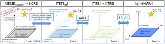
Figure 1. Links between reference systems, coordinate systems, and epochs.

2.1.3. Linking Coordinate Systems: Spherical Trigonometry

Let us consider the celestial sphere and the tangent plane to the reference ellipsoid centered on the observer; see Figure 2. One can build a spherical triangle—defined by P, S, and Z in Figure 2—whose angles depend on the equatorial coordinates of a star at epoch t$(\alpha ,\delta )$, its horizontal coordinates at the same epoch $(A,E)$, the terrestrial coordinates of the observer $(L,\varphi )$, and sidereal time $GAST$. Using this spherical triangle and classical trigonometric formulas [9] (Chapter 13), one can show the following relationships:

$$\left(\mathcal{S}\right):=\left\{\begin{array}{c}H=\mathit{GAST}+L-\alpha ,\hfill \\ sin\left(E\right)=sin\left(\varphi \right)sin\left(\delta \right)+cos\left(\varphi \right)cos\left(\delta \right)cos\left(H\right),\hfill \\ cos\left(A\right)cos\left(E\right)=-cos\left(H\right)sin\left(\varphi \right)cos\left(\delta \right)+sin\left(\delta \right)cos\left(\varphi \right),\hfill \\ sin\left(A\right)cos\left(E\right)=-sin\left(H\right)cos\left(\delta \right).\hfill \end{array}\right.$$

(1)

where $H$ denotes the hour angle of the celestial object. From $\left(\mathcal{S}\right)$, one can easily compute the horizontal coordinates $(A,E)$ of a star of equatorial coordinates $(\alpha ,\delta )$ from a position $(L,\varphi )$. This is what we call the pre-designation of a star:

$$\left\{\begin{array}{c}H=GAST+L-\alpha ,\hfill \\ E=arcsin\left(sin\left(\varphi \right)sin\left(\delta \right)+cos\left(\varphi \right)cos\left(\delta \right)cos\left(H\right)\right),\hfill \\ A=\mathrm{atan}2\left(sin\left(H\right),cos\left(H\right)sin\left(\varphi \right)-tan\left(\delta \right)cos\left(\varphi \right)\right).\hfill \end{array}\right.$$

(2)

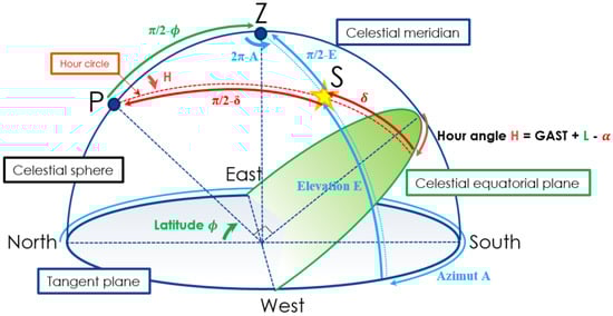
Figure 2. Spherical trigonometry: S—star, P—celestial pole, Z—zenith.

2.2. Estimating the Observer’s Position

System $\left(\mathcal{S}\right)$ can also be seen as equations in the terrestrial coordinates $(L,\varphi )$ for a given observed known star of horizontal coordinates $(A,E)$; this is what we call a star-localization.

Proposition 1.

Let $(L,\varphi )$ be the unknown position of an observer. Let $(\tilde{L},\tilde{\varphi })$ be an assumed position of this observer (for example, computed by an INS in a GNSS-denied environment). Let $(\alpha ,\delta )$ be the equatorial coordinates of a known star at the current epoch t, with $\delta \ne \pm \pi /2$, and $(A,E)$ its theoretical horizontal coordinates obtained from observations from the observer’s position, with $E>0$. Let $GAST$ be the Greenwich Apparent Sidereal Time of the current epoch t. Then, an estimator of the hour angle of this star, deduced from $\tilde{L}$, is defined by:

$$\tilde{H}:=\tilde{L}+\mathit{GAST}-\alpha .$$

(3)

Let $H_0:=\arcsin \left(-{\displaystyle \frac{sin\left(A\right)cos\left(E\right)}{cos\left(\delta \right)}}\right)$. Then, an estimator of the hour angle of the star $H$, deduced from the observed star, is given by

$$\widehat{H}:=\left\{\begin{array}{cc}{H}_0\hfill & \mathit{if}{\left(H_0-\tilde{H}\right)}^2<{\left(\pi -H_0-\tilde{H}\right)}^2,\hfill \\ \pi -H_0\hfill & \mathit{otherwise}.\hfill \end{array}\right.$$

(4)

Furthermore, an estimator of the observer’s position—deduced from the observed star—is given by:

$$\left\{\begin{array}{c}\widehat{L}:=\widehat{H}-\mathit{GAST}+\alpha ,\hfill \\ \widehat{\varphi }:=\arcsin \left({\displaystyle \frac{sin\left(\delta \right)sin\left(E\right)-cos\left(A\right)cos\left(E\right)cos\left(\delta \right)cos(\widehat{H})}{1-sin{\left(A\right)}^{2}cos{\left(E\right)}^2}}\right).\hfill \end{array}\right.$$

(5)

2.3. Sensitivity Analysis of the Localization Problem

Equation (5) is a closed-form estimator of the observer’s position $(L,\varphi )$ from the observed coordinates of a single star. In practice, for each star-sighting, we notice that we obtain a different estimate of position $(\widehat{L},\widehat{\varphi })$. Moreover, with many stars being observable in the sky, one could wonder which star is the best candidate to find one’s position from a single observation. The following proposition provides information on this question by computing a sensitivity analysis of system of Equation (2), linking the observer’s position and their observations with spherical trigonometry.

Proposition 2.

Consider an observer at terrestrial coordinates $(L,\varphi )$, equipped with a clock synchronized on UTC, and able to compute $\mathit{GAST}$ with an accuracy $\mathrm{d}\mathit{G}\mathit{A}\mathit{S}\mathit{T}$. The observer is pointing at stars of theoretical horizontal coordinates $(A,E)$ with an error $(\mathrm{d}A,\mathrm{d}E)$. We assume that the observer has a perfect knowledge of these stars in $\left[{\mathrm{TETE}}_{\left(\mathrm{t}\right)}\right]$, i.e., that the equatorial coordinates $(\alpha ,\delta )$ of all stars have no error. For example, using the NOVAS astronomy software, one can compute these coordinates with an accuracy below 1 mas [10]). We also consider that the following conditions hold for each observation:

(A) 

$\delta \ne \pm \pi /2$, i.e., the star is not at a celestial pole;

(B) 

$H\ne \pm \pi /2$, or equivalently $sin\left(A\right)cos\left(E\right)\ne \pm cos\left(\delta \right)$;

(C) 

$1-sin{\left(A\right)}^{2}cos{\left(E\right)}^2\ne 0$ (satisfied for $E>0$);

(D) 

$\left|sin\left(E\right)cos\left(H\right)cos\left(\delta \right)+sin\left(\delta \right)cos\left(E\right)cos\left(A\right)\right|\ne 0$.

Under these conditions, the estimation of position varies by a quantity $(\mathrm{d}L,\mathrm{d}\varphi )$, which depends on the observation errors $(\mathrm{d}A,\mathrm{d}E)$ and timing errors $\mathrm{d}GAST$ according to the following expression

$$\left\{\begin{array}{c}\mathrm{d}L={\displaystyle \frac{l_A(A,E,H)}{{\mathrm{\Delta }}_L(A,E,\delta )}}\mathrm{d}A+{\displaystyle \frac{l_E(A,E,H)}{{\mathrm{\Delta }}_L(A,E,\delta )}}\mathrm{d}E-\mathrm{d}GAST,\hfill \\ \mathrm{d}\varphi ={\displaystyle \frac{p_A(A,E,\delta ,H)}{{\mathrm{\Delta }}_{\varphi }(A,E,\delta ,H)}}\mathrm{d}A+{\displaystyle \frac{p_E(A,E,\delta ,H)}{{\mathrm{\Delta }}_{\varphi }(A,E,\delta ,H)}}\mathrm{d}E,\hfill \end{array}\right.$$

(6)

where:

$$\left\{\begin{array}{c}{l}_A(A,E,H):=-\mathrm{sign}(cos\left(H\right))cos\left(A\right)cos\left(E\right),\hfill \\ l_E(A,E,H):=\mathrm{sign}(cos\left(H\right))sin\left(A\right)sin\left(E\right),\hfill \\ {\mathrm{\Delta }}_L(A,E,\delta ):=\sqrt{cos{\left(\delta \right)}^2-sin{\left(A\right)}^{2}cos{\left(E\right)}^2},\hfill \\ p_A(A,E,\delta ,H):=cos\left(E\right)sin\left(A\right){\left(sin\left(E\right)cos\left(H\right)cos\left(\delta \right)+sin\left(\delta \right)cos\left(E\right)cos\left(A\right)\right)}^2,\hfill \\ p_E(A,E,\delta ,H):=-cos\left(E\right)sin\left(\delta \right)cos\left(\delta \right)cos\left(H\right)\left(sin{\left(A\right)}^{2}sin{\left(E\right)}^2-cos{\left(A\right)}^2\right)\hfill \\ +sin\left(E\right)cos\left(A\right)\left(cos{\left(H\right)}^{2}cos{\left(\delta \right)}^2-cos{\left(E\right)}^{2}sin{\left(\delta \right)}^{2}sin{\left(A\right)}^2\right),\hfill \\ {\mathrm{\Delta }}_{\varphi }(A,E,\delta ,H):=\left(1-sin{\left(A\right)}^{2}cos{\left(E\right)}^2\right)cos\left(H\right)cos\left(\delta \right)\hfill \\ \left|sin\left(E\right)cos\left(H\right)cos\left(\delta \right)+sin\left(\delta \right)cos\left(E\right)cos\left(A\right)\right|.\hfill \end{array}\right.$$

Remark 1.

Assuming that $(\alpha ,\delta )$ have no error is a reasonable assumption in most cases as most astronomy software is able to compute equatorial coordinates of stars in $\left[{\mathrm{TETE}}_{\left(\mathrm{t}\right)}\right]$ with a high accuracy.

The sensitivity factors $({\displaystyle \frac{l_A}{{\mathrm{\Delta }}_L}},{\displaystyle \frac{l_E}{{\mathrm{\Delta }}_L}},{\displaystyle \frac{p_A}{{\mathrm{\Delta }}_{\varphi }}},{\displaystyle \frac{p_E}{{\mathrm{\Delta }}_{\varphi }}})$ can be used to discriminate stars in order to seek one’s position on the Earth. For a given sighting error, high sensitivity factors tend to amplify the error made on the localization estimation, while low sensitivity factors tend to minimize this error. These sensitivity factors are illustrated, with colors indicating their values, in Figure 3, where we plot $({\displaystyle \frac{l_A}{{\mathrm{\Delta }}_L}},{\displaystyle \frac{l_E}{{\mathrm{\Delta }}_L}},{\displaystyle \frac{p_A}{{\mathrm{\Delta }}_{\varphi }}},{\displaystyle \frac{p_E}{{\mathrm{\Delta }}_{\varphi }}})$ for a given value of $E$, using (6) and:

$$cos\left(H\right)=\mathrm{sgn}\left(H\right){\displaystyle \frac{\sqrt{cos{\left(\delta \right)}^2-sin{\left(A\right)}^{2}cos{\left(E\right)}^2}}{cos\left(\delta \right)}}.$$

(7)

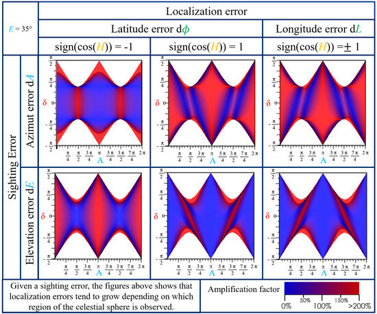
Figure 3. Sensitivity factors for $E={35}^{\circ }$.

As we can remark in Figure 3, some stars may be favorable for estimating latitude, others may be favorable for estimating longitude.

3. Results

In order to verify the relevance of expressions $\mathrm{d}L$ and $\mathrm{d}\varphi$ to estimate an observer’s position using star-sightings, we used the experimental setup described below.

3.1. Experimental Setup

A Safran Electronics & Defense (SED) gyrostabilized sighting device called PASEO XLR^®, an extra long-range optronic identification and fire control system, was used to carry out the observations; see Figure 4a. This system is an electromechanical stabilized system embedding a set of imagers (TV, IR, SWIR, …), optical zooms, and spotters; an inertial measurement unit (IMU) based on hemispherical resonating gyroscopes HRG Crystal^™; and a target tracker. In this experiment, the IMU is mainly used as an Attitude Heading Reference System (AHRS), which provides an estimate of the direction of north and the local vertical. This IMU is also coupled with a GPS receiver, which provides UTC. Images are then recorded at 50 FPS, and a UTC timestamp is associated with the beginning of the exposure of each image with a precision of a few µs. The system also integrates a tracking system, i.e., algorithms able to determine the position of a star in each image (stars being considered as a point spread function), and an attitude control mode, i.e., an option to pilot the sight using position references in azimuth and elevation. Then, the sight is able to reach a precise target on the celestial sphere and to follow it, i.e., to center the identified gray stain in the image by adjusting its azimuth and elevation angles.

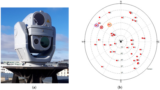
Figure 4. Experimental setup and observations. (a) SED’s sighting device PASEO XLR^® used to carry out the observations. (b) Position on the celestial sphere of the 42 observed stars.

3.2. Observations

Observations were performed at the SED site of Massy, on 9 February 2023, around 17h UTC. We assume that we perfectly know the location of this site, i.e., its geographic coordinates $(L^{★},{\varphi }^{★})$, and we would like to estimate them using star-sightings.

To this end, a set of 42 stars were successively observed, and their location on the celestial sphere is depicted in Figure 4b. This figure shows that our 42 observations cover a large part of the celestial sphere, and are a good basis for validating our algorithms.

Practically, apparent horizontal coordinates $(A_k,E_k)$ of each star are computed using the measures of the AHRS, the tracking estimated errors expressed in pixels, a refraction model taken from [9] (Chapter 16), and some sensor harmonization parameters modeling the misalignment between the optical sensor and the IMU. These harmonization parameters are estimated before starting the observations using a methodology developed at SED (it is not developed here as this is not the purpose of this paper), and introduce some error in computing the apparent position of the star from the measurements.

3.3. Application Results

For each observation k, consisting of apparent horizontal coordinates $(A_k,E_k)$, equatorial coordinates $({\alpha }_k,{\delta }_k)$, and a UTC timestamp, we can compute an estimate of the sight’s position $(\widehat{L_k},\widehat{{\varphi }_k})$ using (5).

The error between the true position of the sight $(L^{★},{\varphi }^{★})$ and the estimated one $(\widehat{L_k},\widehat{{\varphi }_k})$ is denoted by ${\mathit{ϵ}}_{\mathit{k}}:=\left(L^{★}-\widehat{L_k},{\varphi }^{★}-\widehat{{\varphi }_k}\right).$

We then compare two sets of results. In the first set, the apparent horizontal coordinates $(A_k,E_k)$ are computed using biased harmonization parameters modeling the misalignment between the star sensor and the IMU, and thus introduce significant sighting errors. In the second one, we use a minimum-bias methodology to compute these parameters, and thus the sighting errors are reduced.

Figure 5 shows, for each observation, the location error ${\mathit{ϵ}}_{\mathit{k}}$ (between the true position of the sight and the estimated one)—scaled by a secret factor for confidentiality reasons—with the sensitivity factors $({\displaystyle \frac{l_A}{{\mathrm{\Delta }}_L}},{\displaystyle \frac{l_E}{{\mathrm{\Delta }}_L}},{\displaystyle \frac{p_A}{{\mathrm{\Delta }}_{\varphi }}},{\displaystyle \frac{p_E}{{\mathrm{\Delta }}_{\varphi }}})$ for each observation.

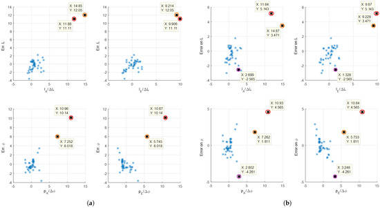
Figure 5. Correlation between the sensitivity factors $({\displaystyle \frac{l_A}{{\mathrm{\Delta }}_L}},{\displaystyle \frac{l_E}{{\mathrm{\Delta }}_L}},{\displaystyle \frac{p_A}{{\mathrm{\Delta }}_{\varphi }}},{\displaystyle \frac{p_E}{{\mathrm{\Delta }}_{\varphi }}})$ (unitless) and location error (normalized) for each observation. (a) Using biased harmonization parameters. (b) Using minimum-biased harmonization parameters. Remarkable stars are circled with color, as in Figure 4b.

4. Discussion

We can notice that the stars with high sensitivity factors provide a bad location estimate. This fact is even clearer when we use the worst harmonization parameters (Figure 5a). However, the contrary may not be true: the stars with the lowest sensitivities do not return the best location estimates. Non-stationary errors, such as those caused by atmospheric refraction modeling or the AHRS’s reference frame, may explain this dispersion. This will be investigated in future work. However, an interesting result is that an observer seeking their position should point at stars with low sensitivity factors, as they tend to return better results.

5. Conclusions

In this paper, we formulated the problem of recovering an observer’s position from celestial observations using spherical trigonometry and we derived sensitivity factors, providing information on how sensing errors affect an estimate of position. These sensitivity factors can be used to discriminate stars, as high sensitivity factors lead to high location errors. This can be useful to reduce the time needed to estimate an observer’s position, for example, in a GNSS-denied environment, as one needs less star-sightings to deduce a good location estimate with good confidence. Furthermore, the sensitivity factors are compact closed-form expressions, and thus are easily embeddable.

6. Patents

The results given in this article are protected under the patent [12] and should not be used for commercial purposes without the knowledge of Safran Electronics & Defense.

References

- Umland, H. A Short Guide in Celestial Navigation; under GNU Free Documentation License. 2019. Available online: https://www.celnav.de/ (accessed on 14 February 2026).
- Liebe, C.C. Star trackers for attitude determination. IEEE Aerosp. Electron. Syst. Mag. 1995, 10, 10–16. [Google Scholar] [CrossRef]
- Samaan, M.; Mortari, D.; Junkins, J.L. Compass Star Tracker for GPS Applications. IEEE Trans. Aero. Elec. Syst. 2008, 118, 75–86. [Google Scholar] [CrossRef]
- Wei, X.; Cui, C.; Wang, G.; Wan, X. Autonomous positioning utilizing star sensor and inclinometer. Measurement 2019, 131, 132–144. [Google Scholar] [CrossRef]
- Ali, J.; Changyun, Z.; Jiancheng, F. An algorithm for astro-inertial navigation using CCD star sensors. Aerosp. Sci. Technol. 2006, 10, 449–454. [Google Scholar] [CrossRef]
- Kopeikin, S.; Efroimsky, M.; Kaplan, G.H. Relativistic Celestial Mechanics of the Solar System; John Wiley & Sons: Hoboken, NJ, USA, 2011. [Google Scholar]
- Bureau des Longitudes. Éphémérides Astronomiques, Connaissance des Temps; IMCCE & EDP Sciences: Les Ulis, France, 2012. [Google Scholar]
- Vallado, D.A. Fundamentals of Astrodynamics and Applicattions, 4th ed.; Microcosm Press: Hawthorne, CA, USA; Springer: Berlin/Heidelberg, Germany, 2013. [Google Scholar]
- Meeus, J. Astronomical Algorithms, 2nd ed.; Atlantic Books: London, UK, 1998. [Google Scholar]
- Bangert, J.; Puatua, W.; Kaplan, G.H.; Bartlett, J.; Harris, W.; Fredericks, A.; Monet, A. User’s Guide to NOVAS Version C3.1; USNO: Washington, DC, USA, 2011. [Google Scholar]
- IAU SOFA Software Collection. Available online: http://www.iausofa.org (accessed on 11 April 2025).
- Rance, G.; Élie, P. Detection and Correction of Drift in a Star Tracking Navigation Device. Patent WO2024089353, 2 May 2024. [Google Scholar]
Disclaimer/Publisher’s Note: The statements, opinions and data contained in all publications are solely those of the individual author(s) and contributor(s) and not of MDPI and/or the editor(s). MDPI and/or the editor(s) disclaim responsibility for any injury to people or property resulting from any ideas, methods, instructions or products referred to in the content. |
© 2026 by the authors. Licensee MDPI, Basel, Switzerland. This article is an open access article distributed under the terms and conditions of the Creative Commons Attribution (CC BY) license.