Abstract
The Inverse Finite Element Method (iFEM) is a valuable tool for reconstructing displacement fields from strain measurements, making it ideal for structural health monitoring. Traditional iFEM approaches are deterministic and typically require dense sensor networks for accurate results. However, practical constraints—such as limited sensor placement and cost—call for robust extrapolation techniques to estimate strain in non-instrumented regions. This paper proposes a stochastic 1D iFEM framework that integrates uncertainty quantification into the strain extrapolation process. By assigning confidence weights to extrapolated values, the method enhances the reliability of displacement reconstruction in sparsely instrumented structures. The approach is validated through numerical and experimental studies, demonstrating improved accuracy and robustness compared to traditional interpolation methods, even under varying loading conditions. The results confirm the method’s suitability for real-world applications in aerospace, civil, and naval engineering, particularly when direct strain measurements are limited.
1. Introduction
Civil infrastructures such as bridges, and naval and aerospace structures, are subjected to heavy loads, environmental changes, and aging. Failures in these systems can be critical, making early detection essential. Structural Health Monitoring (SHM) offers a continuous, sensor-based alternative to traditional Non-Destructive Testing (NDT), which relies on manual inspections [1,2]. SHM enhances safety and serviceability throughout a structure’s life.
A key performance indicator is deflection, which reflects structural deformation under load. Shape sensing, or displacement monitoring, has gained attention for assessing structural behavior. However, direct displacement measurements are often challenging due to the need for accurate models, boundary conditions, and environmental constraints. Traditional methods—such as LVDTs, GPS, radar, photogrammetry, lasers, and inertial sensors [3]—face issues like weather sensitivity, calibration complexity, and limited resolution.
To address these limitations, reference-free approaches have emerged [4], using strain data to estimate deformation. Among them, the inverse Finite Element Method (iFEM) stands out as a powerful tool to reconstruct full-field displacements from sparse strain measurements [5]. Unlike standard FEM, which derives strain from displacements, iFEM works in reverse, enabling displacement estimation without detailed knowledge of loads or material properties.
Under the assumption of linear structural behavior, iFEM requires only the meshed geometry and boundary conditions—without the need for external loads or material properties—making it ideal for scenarios with stochastic or unpredictable loading. It is particularly suited for 1D structures like bridges, where sensor placement is constrained. In this context, distributed strain sensing technologies such as Fiber Bragg Grating (FBG) sensors are gaining traction due to their high spatial resolution and continuous measurement capability.
A key limitation of the 1D iFEM is the need for two strain measurements per element, which can increase costs and vulnerability to sensor failure. To mitigate this, several interpolation and extrapolation techniques have been proposed. Among them, the Smoothing Element Analysis (SEA) method [6] allows for a reduced number of sensors while preserving accuracy. However, extrapolated data should be weighted less than direct measurements, as they carry greater uncertainty.
To solve this problem, the framework followed in this paper is inspired by the method proposed in [7], where the authors use the Gaussian Process (GP) as a strain interpolation/extrapolation technique for 2D shell structures. GPs are a statistical tool that, based on the available data, can estimate the value of a function at points where we have no sensors. GP regression offers several advantages in this context: it is non-parametric, capable of approximating any continuous function and it naturally yields uncertainty estimates alongside predictions [8]. The definition of the uncertainty in the extrapolated strains is a crucial point of this work. Their value will be key in determining how much the extrapolated strains must be considered with respect to the sensor’s strains, like done in [7]. The link between iFEM and GP is made through an appropriate definition of what are called weights. If a predicted strain comes with high uncertainty, it will be given less importance in the reconstruction process (with lower weight). This allows for a more robust and realistic displacement estimation, especially in cases where sensor data is missing or incomplete. Moreover, the GP’s predictive distribution—mean and confidence intervals—can be propagated through iFEM to estimate both the expected displacement field and its un-certainty.
This approach, which is still in its preliminary stages, can help future developments in SHM, like damage detection in real time and studying how changes in materials, loads, or structure geometries affect the structural displacement response.
2. Methodology
2.1. The 1D Inverse Finite Element Method
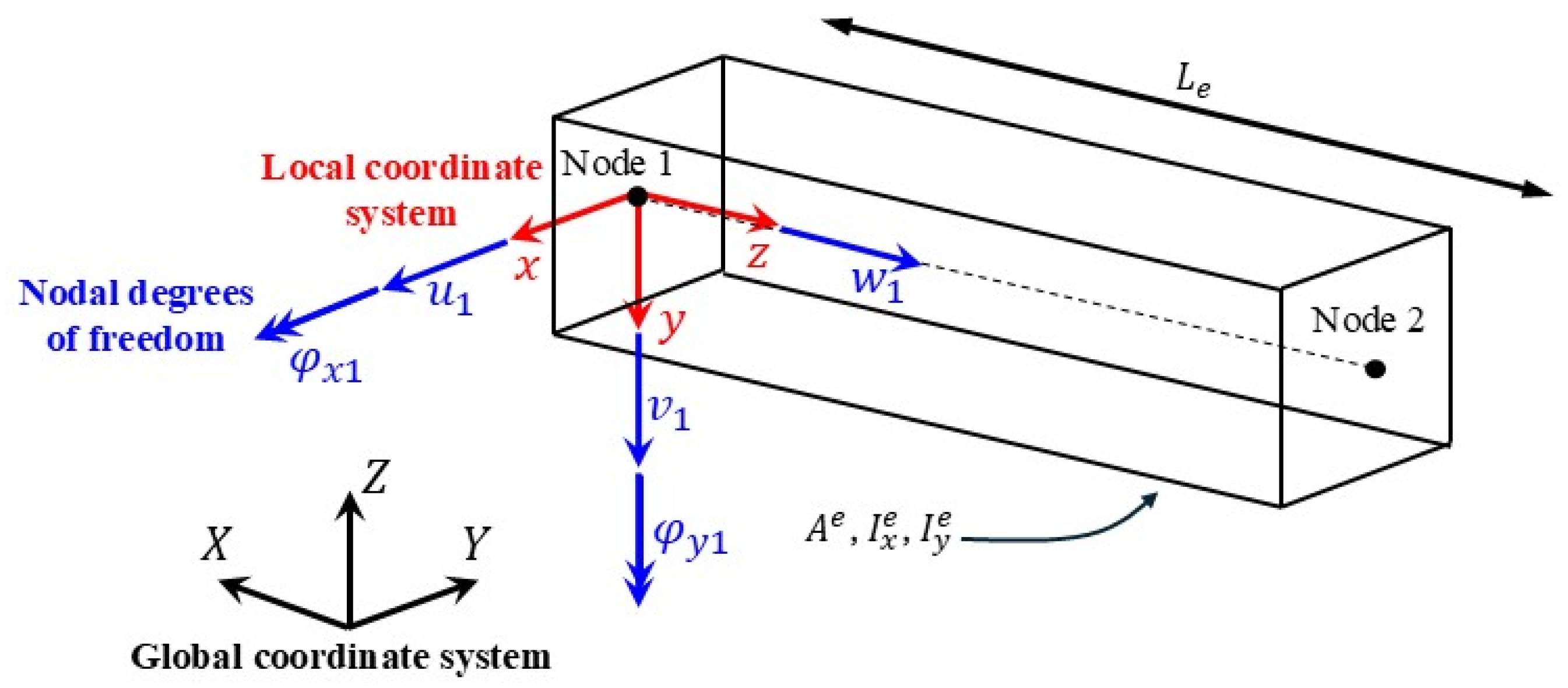
The 1D structure can be discretized with inverse beam elements making use of the zero order Euler-Bernoulli inverse beam elements developed in [4,9]. An illustration of the element with the coordinate system is depicted in Figure 1. According to the Euler-Bernoulli kinematic theory, the only non-null strain component is the strain in direction. These quantities are denoted as section strains and grouped into the strain vector . The components are, respectively, the axial strain and the two curvatures around the and axes.
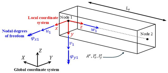
Figure 1.
Illustration of an iFEM element with local and global coordinate systems.
To reconstruct the displacement field from experimentally measured section strains, the iFEM approach minimizes the least-square functional formulated for each element. It consists of the Euclidean norm of the error between the section strains according to the Euler-Bernoulli beam theory and the experimentally measured strains .
Leaving aside all the mathematical steps which can be viewed for further clarification in [4,5], the least-square function can be written as:
where embeds nodal degrees of freedom of the element, is a constant matrix and only depends on the geometry of the element, while the is a column vector that depends on the measured strain data . The minimization result of is analytical, yielding the following linear system of equations:
It is important to notice that the only member dependent on the strain measurements is , but also the term is depended on the weights associated with each single measure.
2.2. Gaussian Process
In this work, a GP is adopted as a probabilistic strain interpolation and extrapolation method within the iFEM framework [10]. The GP leverages prior knowledge from analytical models to estimate the strain field with quantified uncertainty, based on a limited set of sensor measurements.
A GP is defined by a mean function and a covariance function [11]:
where denotes a latent function drawn from the Gaussian Process prior, while is the expectation operator. and are generic input vectors or covariates, whereas represents the covariates at output location. The kernel (covariance function) choice determines the prior knowledge on the function’s smoothness and is governed by hyperparameters [12], typically optimized via Maximum Likelihood Estimation (MLE) [7]. The typical choice in GPs and the one adopted in this paper is the so-called squared exponential (SE) kernel, which is infinitely differentiable, and it has successfully been applied to modeling strains [13].
where and are the kernel hyperparameters. Specifically, represents the signal variance, i.e., how much the data is explained by noise and is the correlation length and represents how rapidly the correlation between the inputs decreases.
It should be noted, however, that the assumptions of smoothness and stationarity may not always be appropriate for modeling strain fields. Further investigations can be performed in the choice of the most appropriate kernel [14], as in the case of compositional kernels search [15].
Once the measurements are made, the Bayes’ theorem is applied to evaluate the distribution of the function conditioned on our observed measurements . The is a set of possibly noisy measurements, the input location ad is the reconstructed function [7,13]. Since all the variables in a Gaussian process have a joint distribution, it does not matter whether these variables have been observed or not. Considering the function value at an unseen data point and the prior distribution (to simplify notation, the mean function is here taken to be zero, which can be performed without loss of generality), the joint distribution of and the noisy measurements can be:
The final goal is finding the posterior distribution of the prediction conditioned on the measured values:
where is a vector containing the mean values for all predicted points and is a matrix encoding the covariance between all predictions. The variance of each predicted point can be extracted considering the diagonal of the matrix .
2.3. Combining iFEM and Gaussian Process
As seen in the introduction section, the principal goal of this paper is using the output of the GRP as a metric to set in an appropriate way the weights associated with each measurement point to be used as input to the iFEM code.
The absolute difference between the higher percentile and the lower percentile of the confidence intervals can be computed for each point :
is a measure of the uncertainty of the interpolation/extrapolation and thus they represent also a metric that can be used to assign the functional weights. Lower weight is assigned for points where the strain has a higher uncertainty with respect to points where the uncertainty is lower. The approach is like the one performed in [7], but with some improvements for this specific application.
For each considered point (extrapolated and measured) a constant is defined as:
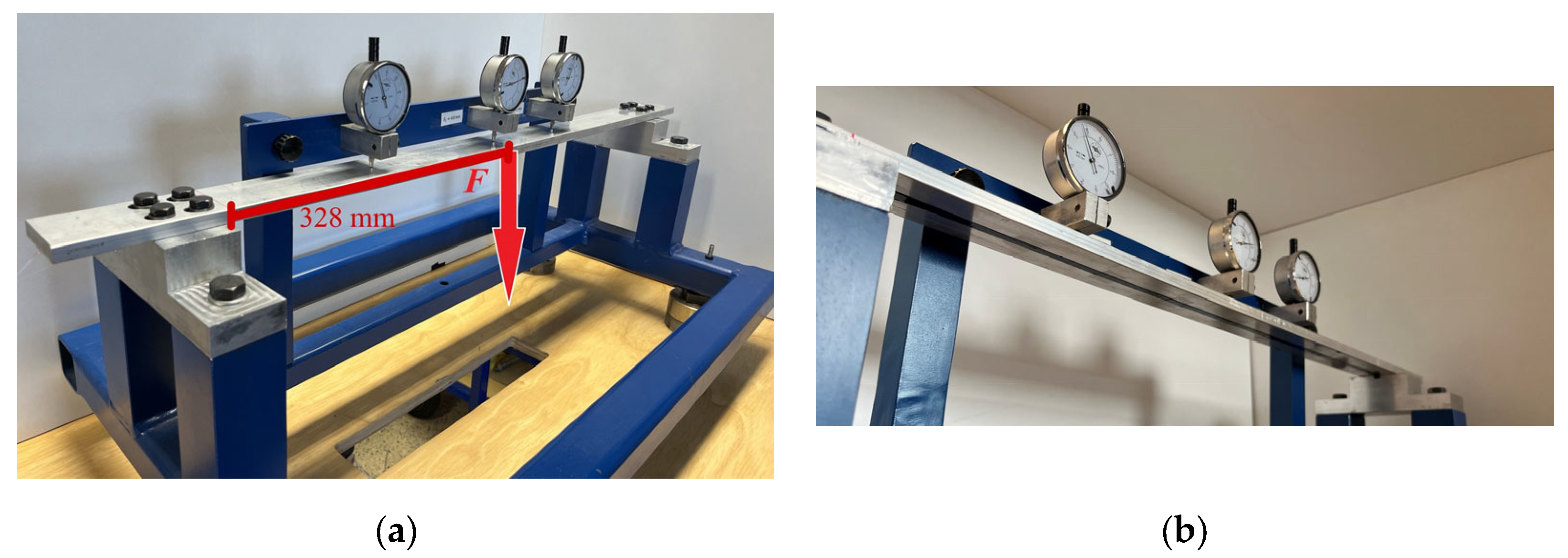
As can be seen in Figure 2b, an uncertainty appears also for the measured point case (it is not perfectly equal to zero for the presence of noise). Therefore, all the vectors are translated using Equation (10).
Here, is a scalar value assigned to each point , while denotes the maximum value among all points in the considered domain (both measured and extrapolated). This normalization guarantees that the measured strain points are assigned , whereas extrapolated points obtain proportionally lower values depending on their associated uncertainty.
As a last step, this paper makes use of a max-min normalization technique to normalize each of and calculate the weight :
It is important to note that the process must be repeated for all strain components (in this specific case for membrane strain and curvature).
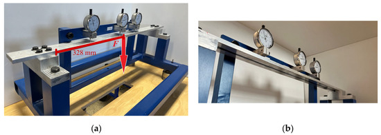
Figure 2.
(a) Experimental setup. (b) Zoom on FBG installed at the bottom of the beam.
Figure 2.
(a) Experimental setup. (b) Zoom on FBG installed at the bottom of the beam.
3. Case Study
In the present paragraph, a brief description of the case under investigation is discussed, with a focus on the experimental test, on the sensor network and on the inverse model.
3.1. Experimental Test
To validate the proposed framework, the geometry of a simple aluminum beam was adopted, featuring a rectangular cross-section with a base of and a height of , and a support span of. The aluminum has the following mechanical properties: Young’s modulus E equal to and Poisson’s ratio υ equal to .
In this framework, three analyses were carried out employing different types of sensor networks, as shown in Table 1. Additionally, the analysis was extended by comparing the Gaussian Process Regression (GPR) with an alternative extrapolation technique, the Cubic Hermite spline (CHS). For each interval between two sensors, the CHS approach constructs a piecewise cubic function using both the measured strain values and the first derivatives estimated through finite differences based on adjacent sensor data. This piecewise cubic function uses Hermite shape functions, which ensure that the interpolation matches both the strain values and their slopes at the sensors, providing smooth transitions between intervals.

Table 1.
Experimental data for different sensor network conditions.

Figure 3.
FBG-based sensor network.
Figure 3.
FBG-based sensor network.

For all the trials, as depicted in Figure 2a, a clamp-clamp boundary condition (BC) scheme is adopted using four screws for each side and a concentrated load equal to is placed at a distance equal to , respect to the left BC.
3.2. The Sensor Network
An FBG-based sensor network was assumed, consisting of 18 measurement points spaced apart (Figure 3). The sensors were positioned along the centreline of the bottom surface of the beam. Each FBG was aligned with the longitudinal axis of the beam and therefore measured the longitudinal strain component, which is the non-null strain component in the Euler–Bernoulli beam formulation considered in this work.
3.3. The Inverse FE Model
The iFEM model of the beam consists of nine 1D inverse finite elements based on the Euler-Bernoulli formulation where each element has a length Le of . According to the formulation of the 0th-order Euler-Bernoulli inverse finite element [4,5], two measurement points are defined within each element. These are symmetrically positioned at one quarter and three-quarters of the element length, to provide optimal strain information for reconstructing the section strain components. It is important to notice that the sensor network introduced in the previous section match perfectly these points. As shown in Table 1, in the second and third case, nine strains value must be pre-extrapolated; in these two cases the GPR and the CHS are used to predict the strains in the point where the sensors are not placed. The same iFEM implementation is performed for the three cases derived from the GPR output: low percentile (LP), high percentile (HP) and mean values.
4. Results and Discussion
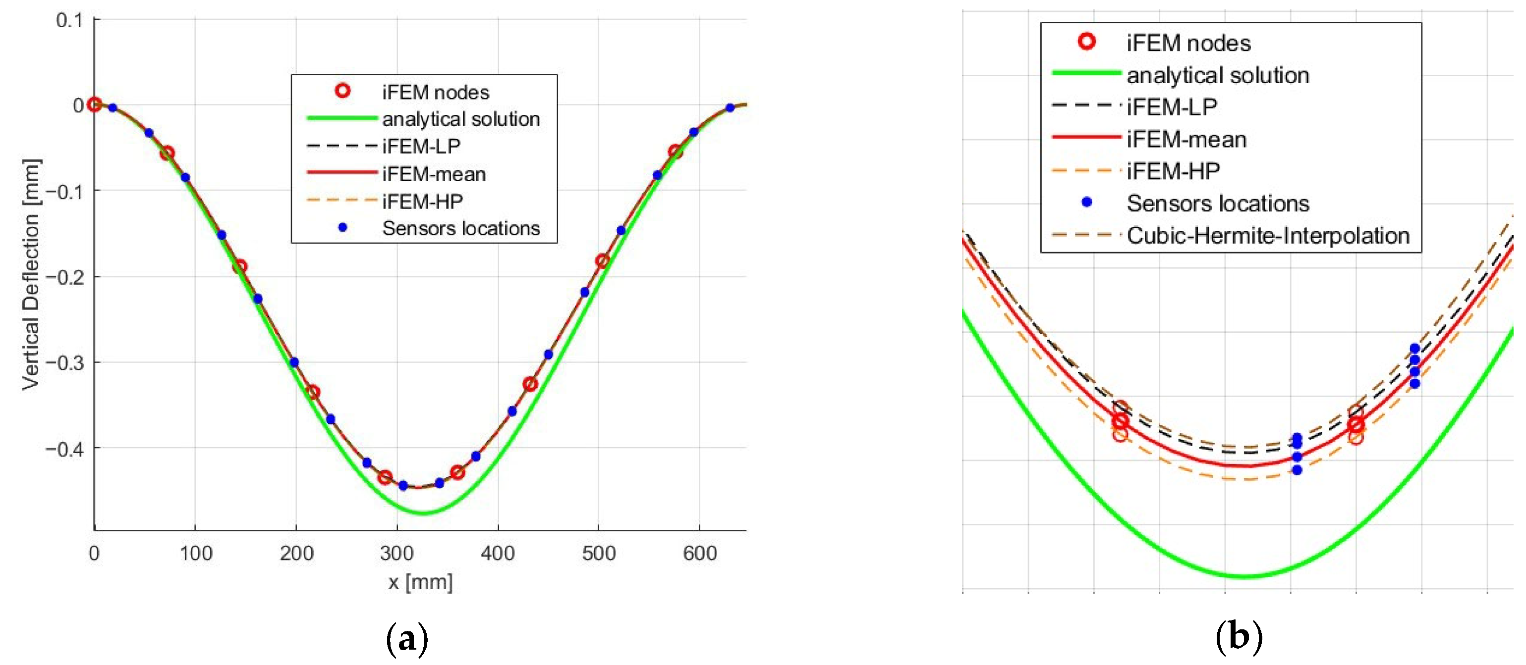
As can be observed from Figure 4a, for the fully instrumented case (Trial 1 with 18 sensors), both GPR and Hermite interpolation provide very similar displacement fields, with a mean-percent difference (MPD) of about 6.5% compared to the analytical solution. This indicates that when sufficient data is available, the choice of extrapolation scheme plays a minor role.

Figure 4.
(a) Displacement field of Trial 1. (b) Displacement field of Trial 2.
In the second case (Trial 2, with only nine sensors), the difference between the schemes becomes more evident. The GPR-based reconstruction yields an MPD of 6.7%, whereas Hermite interpolation results in a larger error of 9.4%. This confirms that the statistical nature of GPR provides more reliable predictions in sparsely instrumented scenarios. Moreover, the uncertainty intervals produced by GPR are relatively narrow, suggesting a consistent level of confidence in the reconstructed strain field. The limited width of these intervals is linked to the smoothness of the squared exponential kernel, which effectively captures the correlation structure of the strain distribution.
Regarding the implementation of the stochastic iFEM, the distribution of the functional weights plays a key role. In the present demonstration, measured strain points were assigned weights close to unity, while extrapolated strains were attributed proportionally smaller values depending on their uncertainty (as defined in Equations (9)–(11)). This weighting strategy allowed the method to preserve the reliability of directly measured data while still leveraging extrapolated values to fill non-instrumented regions. The outcome is a reconstruction that remains robust even under reduced sensor availability, showing the practical applicability of the proposed framework.
5. Conclusions
This study demonstrated the effectiveness of combining 1D iFEM with GPR to accurately reconstruct displacement fields. By enabling strain interpolation with quantified uncertainty, the proposed method overcomes limitations associated with missing sensor data. The GPR-based weighting strategy enhances both the robustness and accuracy of the reconstruction, outperforming traditional interpolation and extrapolation techniques. The validity of the approach was confirmed through both numerical simulations and experimental tests.
Author Contributions
Conceptualization, J.B.; methodology, J.B., R.M., E.P., G.A., A.M. and C.S.; software, J.B.; validation, J.B.; formal analysis, J.B.; investigation, J.B., C.S. and A.M.; resources, J.B., C.S. and A.M.; data curation, J.B.; writing—original draft preparation, J.B., C.S. and A.M.; writing—review and editing, J.B., C.S. and A.M.; visualization, J.B.; supervision, C.S. and A.M. All authors have read and agreed to the published version of the manuscript.
Funding
This research received no external funding.
Institutional Review Board Statement
Not applicable.
Informed Consent Statement
Not applicable.
Data Availability Statement
The data presented in this study are available on request from the corresponding author.
Conflicts of Interest
The authors declare no conflicts of interest.
References
- Worden, K.; Cross, E.J.; Dervilis, N.; Papatheou, E.; Antoniadou, I. Structural Health Monitoring: From Structures to Systems-of-Systems. IFAC-PapersOnLine 2015, 48, 1–17. [Google Scholar] [CrossRef]
- Pallarés, F.J.; Betti, M.; Bartoli, G.; Pallarés, L. Structural Health Monitoring (SHM) and Nondestructive Testing (NDT) of Slender Masonry Structures: A Practical Review. Constr. Build. Mater. 2021, 297, 123768. [Google Scholar] [CrossRef]
- Ma, Z.; Choi, J.; Sohn, H. Structural Displacement Sensing Techniques for Civil Infrastructure: A Review. J. Infrastruct. Intell. Resil. 2023, 2, 100041. [Google Scholar] [CrossRef]
- Poloni, D.; Morgese, M.; Wang, C.; Taylor, T.; Giglio, M.; Ansari, F.; Sbarufatti, C. Reference-Free Distributed Monitoring of Deflections in Multi-Span Bridges. Eng. Struct. 2025, 323, 119277. [Google Scholar] [CrossRef]
- Savino, P.; Gherlone, M.; Tondolo, F. Shape Sensing with Inverse Finite Element Method for Slender Structures. Struct. Eng. Mech. 2019, 72, 217–227. [Google Scholar] [CrossRef]
- Oboe, D.; Colombo, L.; Sbarufatti, C.; Giglio, M. Comparison of Strain Pre-Extrapolation Techniques for Shape and Strain Sensing by iFEM of a Composite Plate Subjected to Compression Buckling. Compos. Struct. 2021, 262, 113587. [Google Scholar] [CrossRef]
- Poloni, D.; Oboe, D.; Sbarufatti, C.; Giglio, M. Towards a Stochastic Inverse Finite Element Method: A Gaussian Process Strain Extrapolation. Mech. Syst. Signal Process. 2023, 189, 110056. [Google Scholar] [CrossRef]
- Rasmussen, C.E.; Williams, C.K.I. Gaussian Processes for Machine Learning, 1st ed.; MIT Press: Cambridge, MA, USA, 2005. [Google Scholar] [CrossRef]
- Gherlone, M.; Cerracchio, P.; Mattone, M.; Di Sciuva, M.; Tessler, A. An Inverse Finite Element Method for Beam Shape Sensing: Theoretical Framework and Experimental Validation. Smart Mater. Struct. 2014, 23, 045027. [Google Scholar] [CrossRef]
- Ebden, M. Gaussian processes: A quick introduction. arXiv 2015, arXiv:1505.02965. [Google Scholar] [CrossRef]
- Schulz, E.; Speekenbrink, M.; Krause, A. A Tutorial on Gaussian Process Regression: Modelling, Exploring, and Exploiting Functions. J. Math. Psychol. 2018, 85, 1–16. [Google Scholar] [CrossRef]
- Petit, S.J.; Bect, J.; Feliot, P.; Vazquez, E. Parameter Selection in Gaussian Process Interpolation: An Empirical Study of Selection Criteria. SIAM/ASA J. Uncertain. Quantif. 2023, 11, 1308–1328. [Google Scholar] [CrossRef]
- Jidling, C. Strain Field Modelling Using Gaussian Processes. Master’s Thesis, Chalmers University of Technology, Gothenburg, Sweden, 2017. [Google Scholar]
- Abdessalem, A.B.; Dervilis, N.; Wagg, D.J.; Worden, K. Automatic Kernel Selection for Gaussian Processes Regression with Approximate Bayesian Computation and Sequential Monte Carlo. Front. Built Environ. 2017, 3, 52. [Google Scholar] [CrossRef]
- Duvenaud, D.; Lloyd, J.R.; Grosse, R.; Tenenbaum, J.B.; Ghahramani, Z. Structure Discovery in Nonparametric Regression through Compositional Kernel Search. In Proceedings of the 30th International Conference on Machine Learning (ICML), Atlanta, GA, USA, 16–21 June 2013. [Google Scholar] [CrossRef]
Disclaimer/Publisher’s Note: The statements, opinions and data contained in all publications are solely those of the individual author(s) and contributor(s) and not of MDPI and/or the editor(s). MDPI and/or the editor(s) disclaim responsibility for any injury to people or property resulting from any ideas, methods, instructions or products referred to in the content. |
© 2025 by the authors. Licensee MDPI, Basel, Switzerland. This article is an open access article distributed under the terms and conditions of the Creative Commons Attribution (CC BY) license (https://creativecommons.org/licenses/by/4.0/).

