Exploring the Correlation Between Gaseous Emissions and Phenological Phases in Tomato Crops Through Machine Learning ^†

Abstract

Nowadays, agriculture is facing significant challenges, including climate change. Precision agriculture might address these issues by optimizing resource use and promoting sustainability. In this work, a case study of tomato crop monitoring is presented, employing a large amount of gas sensor data collected over three years (2020–2022) to develop models for phenological phase classification. A k-NN classifier achieved accuracies above 99% across multiple train/test splits, with AUC, sensitivity, specificity, precision, and F1-score above 98%. Results demonstrate the feasibility of low-computational-cost systems capable of real-time detection of the transition point between plants’ developmental stages.

1. Introduction

Despite being used for centuries, traditional agricultural methods embody serious drawbacks since they may not be as fruitful or profitable as they once were. Indeed, there is a need for innovative tools for climate adaptation, addressing the growing environmental challenges faced by modern agricultural systems, such as rising temperatures and prolonged periods of drought that are causing a decline in both the quantity and quality of yields. Precision agriculture might be a viable solution, being a modern agricultural approach that uses technology and data analysis to improve farming efficiency. This strategy might optimize resource use, increase production, and promote sustainability. Real-time monitoring and targeted interventions would lead to an effective management of climate-related challenges and economic viability, while minimizing environmental impacts when compared to traditional procedures [1].

Among the crucial empirically derived agronomic parameters, there are phenological phases (Phases) of plants. Phases define stages of a plant’s life cycle and development, marking key stages in crop growth. These stages are mainly influenced by environmental factors, which may be biological, such as diseases, competitions, soil, genetics, age, and pests, or related to meteorological conditions, weather during the current growing season, the previous vegetation period, the dormancy phase, or in connection with photoperiod [2]. Climate change is having an impact on Phases as well, determining the advance of phenological events, making the monitoring of the plant development imperative, as ecosystems are increasingly undergoing climatic alterations [3].

Traditionally, calendar time has been used for predicting the timing of developmental stages. However, this approach has been insufficient due to the dependence of the Phase on multiple external factors. It has been established that there is a relationship between temperature and development rate, enabling fairly accurate predictions of crop phenological development. Thus, models based on temperature explain most of the observed variability in development [4]. However, the methods relying on temperature and energy acquired by the crop might be outdated, as the evaluations of Phases are too sensitive to external factors, as previously mentioned. Therefore, in this work, machine learning (ML) was employed to predict phenological phase transitions directly from plant emission signals acquired with four metal oxide (MOX)-based gas sensors, enabling the identification of odor environments [5] specific to internal physiological markers of the plants. This might overcome the limitations of environmental-based methods by leading to the reconstruction of a signal pattern, enabling the precise detection of the transition point between phenological phases. MOX-based gas sensors have been widely investigated for agro-alimentary applications, from post-harvest control [6] and meat inspection [7] to monitoring food authenticity [8]. These studies highlight the versatility of MOX sensing for monitoring in food and farming contexts, providing a strong framework for our investigation on tomato Phase classification [5] with the use of a previously validated sensor array for precision agriculture, developed in the University of Ferrara Sensors Laboratory [9].

Classification is a supervised learning method in which machine learning algorithms are trained to assign labels to input data based on patterns learned from a labeled training dataset [5]. The main purpose of these methods is to generalize from the training sets such that the model can correctly predict the label of previously unseen data. Indeed, applying machine learning techniques to a wide range of sensor signals may allow us to train a model capable of identifying the phenological phases. In this work, a case study of tomato crop monitoring is presented. Employing a large amount of data collected over the years, we developed a model to perform Phases classification. This exploratory study is based on relatively simple and computationally efficient ML algorithms, and it investigates their performance using a compact set of 10 features with various train/test splits to evaluate the potential for accurate classification with minimal computational complexity.

2. Materials and Methods

From 2020 to 2022, we conducted monitoring campaigns on processing tomato crops, typically from early June to early September. The campaign was a result of a collaboration with the agronomists of Canale Emiliano Romagnolo (CER), at their Acqua Campus, near Budrio (BO), Italy. A graphical representation of the data analysis workflow is depicted in Figure 1.

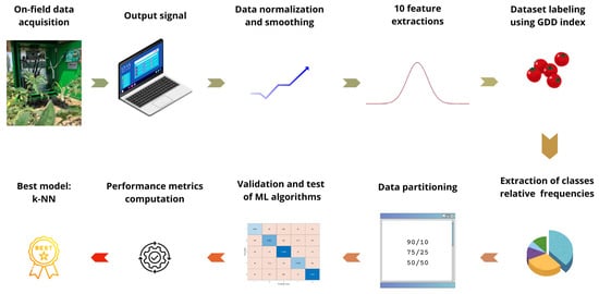
Figure 1. Graphical representation of the data-processing workflow.

Sensing platform. As part of the project, a multifunctional station was installed in a tomato crop field, equipped with the following: a relative humidity (RH%) and temperature sensor (Sensirion SHT11), and four MOX-based gas sensors to monitor plants’ gaseous emissions during their phenological development [9]. In particular, the n-type MOX-based sensors were gold-doped tin dioxide (SnO₂/Au [6]), platinum-doped tin dioxide (SnO₂/Pt [10]), palladium-doped tin dioxide (SnO₂/Pd [6]), and tungsten trioxide (WO₃ [11]), and they were produced and packaged at the Sensors Laboratory at the University of Ferrara. A continuous and real-time measure of the sensors’ signal (mV) was acquired over the whole crop campaign. Exhaustive details on the campaign and on the sensing system can be found in [9].

ML analysis. For tomato crops, it is possible to define 7 Phases: (1) pre-emergence; (2) sowing/transplanting; (3) fruit set–first truss; (4) veraison–first truss; (5) veraison–second truss; (6) ripening: 50% of berries, fully colored; and (7) ripening: 100% of berries, fully colored. The Phases distinctions were based on the Growing Degree Days (GDD) index, which measures the accumulation of heat that is useful for plant growth during the crop cycle, and it was used to mark the transition from one developmental stage to another. With this method, each phenological stage requires a specific amount of thermal energy to be completed, and knowledge of a plant’s specific thermal requirements enables an estimation of the time required to complete each developmental stage. The GDD method was initially employed to label signals within specific time intervals in which data were acquired. The datasets we obtained generally cover Phases from 2 to 6, which were assigned to classification labels ranging from 1 to 5. In the center of Phases, we assumed that we were labeling the correct Phase and that the most significant errors in GDD computations might have occurred at the edge of phenological stages. However, since the distribution of samples across phenological stages is naturally unbalanced, it is not guaranteed that an equal representation of each class will be achieved in the training and test sets. This variability in Phase frequencies might confirm that they should have had more accurate parameters for more represented classes. Consequently, some phenological stages may be underrepresented.

With the large amount of data acquired, the focus can shift from traditional GDD calculations to pattern recognition. Such information is crucial for developing models capable of identifying signal patterns that differentiate between developmental stages, making it possible to find a tool able to distinguish Phases from the input of the plants and not from external features.

The data were analyzed within the MATLAB R2024a environment, and the Classification Learner App was then used to train models for data classification using various supervised machine learning algorithms.

Each sensor’s raw signal, with a measurement acquired every 14 s, contributed to the overall dataset. The raw signals were normalized and then smoothed through the Savitzky–Golay filter [7]. From the pre-processed data, 10 features were extracted: root-mean-square value, standard deviation, mean, minimum, maximum, zero-crossing rate, skewness, kurtosis, range, and median value [7]. Afterward, the data were labeled using the GDD method, and a script was also created to analyze the class frequency distributions across different datasets, ensuring an extensive understanding of class imbalance and its possible impact on model performance.

Subsequently, the model was trained to associate the signal features with their corresponding Phase labels. In order to confirm that the model could accurately identify new, unseen samples, its performance was then tested with the use of a separate dataset. The preliminary analysis was conducted on the dataset acquired during the 2020 campaign, using a five-fold cross-validation (CV) scheme with a 90%/10% train/test split. In this case, the performance of the models could be affected by the natural unbalance in class relative frequency, and thus a study on a cumulative dataset combining 2020, 2021, and 2022 campaigns was conducted, confronting the issue with a more balanced dataset, provided by multiple years of data. Indeed, for the cumulative dataset, the same five-fold CV procedure was used, exploring three train/test split configurations: 90%/10%, 75%/25%, and 50%/50%. These three different partition schemes were examined to explore both the learning capacity and the robustness of the models, i.e., the potentiality of the pattern recognition. Larger training sets support pattern learning, while larger test sets ensure generalized performance. Relatively simple and computationally efficient algorithms were tested, including decision trees, k-nearest neighbors (k-NN), support vector machines, and logistic regression. Among these, the Fine k-NN [12,13,14] classifier achieved the best performance for each validation and test.

To evaluate the performance, each classifier provided the validation accuracy, the test accuracy, the confusion matrix (CM), and the Receiver Operating Characteristic (ROC) curves along with the corresponding Area Under the Curve (AUC) values for each class. ROC curves provide a graphical representation of the classifier’s performance [7], while the computation of various significant metrics for performance was made possible by the analysis of the CM, particularly the identification of true positives (TP), true negatives (TN), false positives (FP), and false negatives (FN). These metrics include sensitivity (R), specificity (S), precision (P), and F1 score (F), defined as follows [15]:

$$\mathrm{R} = {\displaystyle \frac{\mathrm{T}\mathrm{P}}{\mathrm{T}\mathrm{P}+\mathrm{F}\mathrm{N}}}$$

(1)

$$\mathrm{S}={\displaystyle \frac{\mathrm{T}\mathrm{N}}{\mathrm{T}\mathrm{N}+\mathrm{F}\mathrm{P}}}$$

(2)

$$\mathrm{P}={\displaystyle \frac{\mathrm{T}\mathrm{P}}{\mathrm{T}\mathrm{P}+\mathrm{F}\mathrm{P}}}$$

(3)

$$\mathrm{F}=2{\displaystyle \frac{\mathrm{P}·\mathrm{R}}{\mathrm{P}+\mathrm{R}}}$$

(4)

3. Result and Discussion

3.1. Preliminary Study on 2020 Campaign

The class relative frequency distribution for the 2020 campaign reveals a notable imbalance among the classes (Table 1). Specifically, classes 3 and 5 represent the majority of the samples, while classes 1 and 4 are significantly underrepresented. Class 2 also exhibits a lower population.

Table 1. Class distribution for the 2020 campaign dataset. The table reports the relative frequency of samples for each class.

Class	Class Relative Frequency [%]
1	3.15
2	16.93
3	35.41
4	10.10
5	34.40

For the Fine k-NN classifier, high accuracy was achieved in both validation (98.6%) and test (98.8%) phases. The AUC values for the ROC curves ranged between 97% and 99% (Figure 2b), indicating that the algorithm is able to discriminate the correct signal corresponding to the phenological phases, with minimal class overlap [7]. Specifically, the lowest AUC values are observed for Classes 1, 2, and 4, which is consistent with their relatively lower sensitivity, precision, and F1 scores (Table 2). This performance discrepancy can be attributed to the imbalanced distribution of samples across phenological stages. For Classes 3 and 5, the sensitivity, specificity, precision, and F1 score are equal or exceed 99%, demonstrating these classes’ optimal categorization performance. Such an imbalance could be mitigated by collecting data from multiple years, since the temporal distribution of classes varies across years, thereby increasing the representativeness of these phases.

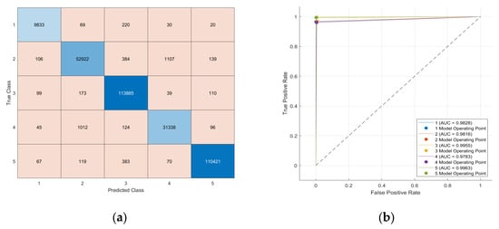
Figure 2. (a) Confusion Matrix (CM) and (b) ROC curves of the Fine k-NN model for the 2020 campaign dataset. In the CM, darker blue tones along the diagonal indicate higher correct classification rates. In the ROC curves, the dotted line represents a random classifier (AUC = 0.5).

Table 2. Performance metrics for each class obtained using the Fine k-NN validation algorithm with a 90%/10% train/test split on the 2020 campaign dataset.

Class	Sensitivity [%]	Specificity [%]	Precision [%]	F1 Score [%]
1	96.7	99.9	96.9	96.8
2	96.8	99.5	97.5	97.1
3	99.6	99.5	99.0	99.3
4	96.1	99.6	96.2	96.1
5	99.4	99.8	99.7	99.5

3.2. Analysis of the Cumulative Dataset (2020–2022)

The class relative frequency distribution in the cumulative dataset (Table 3) shows a more balanced representation compared to the 2020 dataset alone. Classes 3 and 5 remain the most populated, but their frequencies have slightly decreased. Classes 1 and 2 exhibit increased relative frequencies. Notably, for Class 1, the representation of the classes improved from only 3.15% in 2020 to 15.18% in the cumulative dataset. The combination of data from several years improved the balance of the classes, even though Class 4 continues to occur at a relatively low frequency.

Table 3. Class distribution for the cumulative dataset (2020–2022). The table reports the relative frequency of samples for each class.

Class	Class Relative Frequency [%]
1	15.18
2	13.91
3	28.71
4	9.87
5	32.32

Analysis conducted on the cumulative dataset with a 90%/10% train/test split configuration, there were high validation and test accuracies for the Fine k-NN classifier, respectively, 99.6% and 99.8%. The AUC of 99% (Figure 3b) defines an optimal discriminatory power. The performance metrics for all classes demonstrate high values for the calculated metrics (Table 4), all above 98%. In this case, performance is ideal for all classes, despite the 2020 case, in which the less-represented phases had lower metrics. This demonstrates that the model achieves robust classification performance across all classes, including the least represented ones, most likely due to the balance and temporal variety given by multiple years of data. These results indicate that the Fine k-NN validation algorithm performs robustly and reliably across all phenological classes under a 90%/10% train/test split configuration.

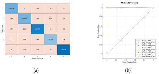
Figure 3. (a) Confusion Matrix (CM) and (b) ROC curves of the Fine k-NN model for the cumulative dataset, using 90%/10% train/test split. In the CM, darker blue tones along the diagonal indicate higher correct classification rates. In the ROC curves, the dotted line represents a random classifier (AUC = 0.5).

Table 4. Performance metrics for each class obtained using the Fine k-NN validation algorithm with a 90%/10% train/test split on the cumulative dataset.

Class	Sensitivity [%]	Specificity [%]	Precision [%]	F1 Score [%]
1	99.8	99.9	99.7	99.8
2	98.9	99.9	99.0	99.0
3	99.8	99.8	99.6	99.7
4	98.7	99.9	98.9	98.8
5	99.8	99.9	99.9	99.8

With a 90%/10% distribution, most of the data are used for the training. As a result, the model can learn more complicated patterns while also being prone to overfitting. Indeed, as a further challenge, it was interesting exploring the 75%/25% train/test split. This split uses an inferior amount of data to train, yet a wider set of tests for algorithm robustness, resulting in a more reliable performance. Moreover, in the absence of strong patterns, the model has less capacity for generalization. Despite this, the performance remains consistently high. Indeed, the Fine k-NN classifier showed high accuracy for both validation and test, respectively, 99.5% and 99.6%, with AUC values from 99% above (Figure 4b). In general, all the metrics being above 98% (Table 5) indicate that the model maintains an optimal classification accuracy and balanced performance across phenological classes, even when a larger fraction of the data is used for testing.

Figure 4. (a) Confusion Matrix (CM) and (b) ROC curves of the Fine k-NN model for the cumulative dataset, using 75%/25% train/test split. In the CM, darker blue tones along the diagonal indicate higher correct classification rates. In the ROC curves, the dotted line represents a random classifier (AUC = 0.5).

Table 5. Performance metrics for each class obtained using the Fine k-NN validation algorithm with a 75%/25% train/test split on the cumulative dataset.

Class	Sensitivity	Specificity	Precision	F1 Score
1	99.7	99.9	99.7	99.7
2	98.8	99.8	98.9	98.9
3	99.8	99.8	99.6	99.7
4	98.5	99.9	98.7	98.6
5	99.8	99.9	99.9	99.8

The most challenging model investigated was the one explored with a 50%/50% train/test split. In this case, the model uses less data for training, which increases the risk of underfitting in the absence of a clear pattern, possibly leading to a decrease in accuracy, while the performance is evaluated rigorously due to the large test set. Despite this, high accuracies were obtained in both validation (99.4%) and test (99.4%), with all AUC being above 99% (Figure 5b). The performance metrics, all above 98% (Table 6), for the 50%/50% train/test split demonstrate strong classification results across all classes, despite the decreased train set size. These results suggest that the model has good generalization capability.

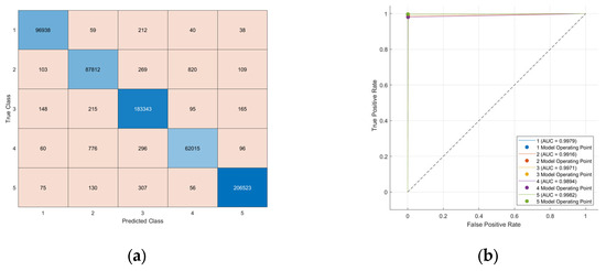
Figure 5. (a) Confusion Matrix (CM) and (b) ROC curves of the Fine k-NN model for the cumulative dataset, using 50%/50% train/test split. In the CM, darker blue tones along the diagonal indicate higher correct classification rates. In the ROC curves, the dotted line represents a random classifier (AUC = 0.5).

Table 6. Performance metrics for each class obtained using the Fine k-NN validation algorithm with a 50%/50% train/test split on the cumulative dataset.

Class	Sensitivity	Specificity	Precision	F1 Score
1	99.6	99.9	99.6	99.6
2	98.5	99.8	98.7	98.6
3	99.7	99.8	99.4	99.5
4	98.1	99.8	98.4	98.2
5	99.7	99.9	99.8	99.8

4. Conclusions

This study demonstrates the potential of precision agriculture to address emerging challenges such as climate change and improve economic viability through machine learning approaches.

The first challenge of the analyzed datasets was the class imbalance, evident in the 2020 data, which resulted in slightly lower performance metrics with still high validation (98.6%) and test (98.8%) accuracies, with AUC values ranging between 97% and 99%, indicating strong discriminatory power. Collecting data from various years minimized this limitation, providing more balanced class distribution. Indeed, analyses on the cumulative dataset (2020–2022 data) showed improved results under three different train/test splits. All three models achieved AUCs above 99%, with performance metrics higher than 98% across all classes. Using a 90%/10% split, the Fine k-NN classifier reached validation and test accuracies of 99.6% and 99.8%, respectively. Similarly, the 75%/25% split yielded validation and test accuracies of 99.5% and 99.6%. Even with the more challenging 50%/50% split, high accuracies were maintained, obtaining 99.4% for both validation and testing.

Indeed, these results show that even with the extraction of only ten features from raw data, these results are highly discriminative between classes. This could be due to a clearly defined pattern separating the phenophases, which can be identified using a relatively simple and computationally efficient algorithm. Moreover, the optimal performances obtained with a 50%/50% split indicate that the model is highly generalizable. This phenomenon is likely attributable to the datasets’ robust representativeness of the classes, as the model maintains high performance even when just half of the data is used for training.

The results of this explorative study are highly encouraging. It has been demonstrated that the olfactory environment of tomato crops is characteristic of each plant’s developmental phase. This carries a high applicative potential, since it might result in the optimization of resource use, such as smarter water management, ensuring economic viability and sustainability, while increasing production efficiency. Since the data may be handled by a very simple algorithm with few feature extractions, it may be possible to create a real-time classification system with basic hardware and with low computational cost.

References

- Mansoor, S.; Iqbal, S.; Popescu, S.M.; Kim, S.L.; Chung, Y.S.; Baek, J.-H. Integration of Smart Sensors and IOT in Precision Agriculture: Trends, Challenges and Future Prospectives. Front. Plant Sci. 2025, 16, 1587869. [Google Scholar] [CrossRef] [PubMed]
- Menzel, A. Trends in Phenological Phases in Europe between 1951 and 1996. Int. J. Biometeorol. 2000, 44, 76–81. [Google Scholar] [CrossRef] [PubMed]
- Czernecki, B.; Nowosad, J.; Jabłońska, K. Machine Learning Modeling of Plant Phenology Based on Coupling Satellite and Gridded Meteorological Dataset. Int. J. Biometeorol. 2018, 62, 1297–1309. [Google Scholar] [CrossRef] [PubMed]
- Slafer, G.A.; Savin, R. Developmental Base Temperature in Different Phenological Phases of Wheat (Triticum Aestivum). J. Exp. Bot. 1991, 42, 1077–1082. [Google Scholar] [CrossRef]
- Stevan, S.L., Jr.; Garcia, A.F.; Menegotto, B.A.; Rocha, J.C.; Siqueira, H.V.; Ayub, R.A. Phenological Stages Analysis in Peach Trees Using Electronic Nose. Open Agric. 2024, 9, 20220337. [Google Scholar] [CrossRef]
- Giberti, A.; Carotta, M.C.; Guidi, V.; Malagù, C.; Martinelli, G.; Piga, M.; Vendemiati, B. Monitoring of Ethylene for Agro-Alimentary Applications and Compensation of Humidity Effects. Sens. Actuators B Chem. 2004, 103, 272–276. [Google Scholar] [CrossRef]
- Shtepliuk, I.; Domènech-Gil, G.; Almqvist, V.; Kautto, A.H.; Vågsholm, I.; Boqvist, S.; Eriksson, J.; Puglisi, D. Electronic Nose and Machine Learning for Modern Meat Inspection. J. Big Data 2025, 12, 96. [Google Scholar] [CrossRef]
- Gliszczyńska-Świgło, A.; Chmielewski, J. Electronic Nose as a Tool for Monitoring the Authenticity of Food. A Review. Food Anal. Methods 2016, 10, 1800–1816. [Google Scholar] [CrossRef]
- Fabbri, B.; Valt, M.; Parretta, C.; Gherardi, S.; Gaiardo, A.; Malagù, C.; Mantovani, F.; Strati, V.; Guidi, V. Correlation of Gaseous Emissions to Water Stress in Tomato and Maize Crops: From Field to Laboratory and Back. Sens. Actuators B Chem. 2020, 303, 127227. [Google Scholar] [CrossRef]
- Lee, Y.-I.; Lee, K.-J.; Lee, D.-H.; Jeong, Y.-K.; Lee, H.S.; Choa, Y.-H. Preparation and Gas Sensitivity of SnO2 Nanopowder Homogenously Doped with Pt Nanoparticles. Curr. Appl. Phys. 2009, 9, S79–S81. [Google Scholar] [CrossRef]
- Cantalini, C.; Wlodarski, W.; Li, Y.; Passacantando, M.; Santucci, S.; Comini, E.; Faglia, G.; Sberveglieri, G. Investigation on the O3 Sensitivity Properties of WO3 Thin Films Prepared by Sol–Gel, Thermal Evaporation and R.F. Sputtering Techniques. Sens. Actuators B Chem. 2000, 64, 182–188. [Google Scholar] [CrossRef]
- Behera, S.K.; Das, A.; Sethy, P.K. Deep Fine-KNN Classification of Ovarian Cancer Subtypes Using Efficientnet-B0 Extracted Features: A Comprehensive Analysis. J. Cancer Res. Clin. Oncol. 2024, 150, 361. [Google Scholar] [CrossRef] [PubMed]
- Hamidi, A.A.; Robertson, B.; Ilow, J. A New Approach for ECG Artifact Detection Using Fine-KNN Classification and Wavelet Scattering Features in Vital Health Applications. Procedia Comput. Sci. 2023, 224, 60–67. [Google Scholar] [CrossRef]
- Liu, X.; Zhang, P.; Guo, Y.; Ma, G.; Liu, M. Study of a High-Precision Complex 3D Geological Modelling Method Based on a Fine KNN and Kriging Coupling Algorithm: A Case Study for Jiangsu, China. Front. Earth Sci. 2023, 11, 1325907. [Google Scholar] [CrossRef]
- Marioriyad, A.; Ramazi, P. Optimizing Accuracy, Recall, Specificity, and Precision Using ILP. Mathematics 2025, 13, 1059. [Google Scholar] [CrossRef]
Disclaimer/Publisher’s Note: The statements, opinions and data contained in all publications are solely those of the individual author(s) and contributor(s) and not of MDPI and/or the editor(s). MDPI and/or the editor(s) disclaim responsibility for any injury to people or property resulting from any ideas, methods, instructions or products referred to in the content. |
© 2025 by the authors. Licensee MDPI, Basel, Switzerland. This article is an open access article distributed under the terms and conditions of the Creative Commons Attribution (CC BY) license (https://creativecommons.org/licenses/by/4.0/).