Bridging Theory and Simulation: Parametric Identification and Validation for a Multirotor UAV in PX4—Gazebo ^†

Abstract

This paper introduces a structured methodology for bridging the gap between theoretical modeling and high-fidelity simulation of multirotor Unmanned Aerial Systems (UAS) through the construction of digital twins in PX4 v1.12 Software-in-the-Loop (SITL) environments. A key challenge addressed is the absence of standardized procedures for translating physical UAV characteristics into simulation-ready parameters, which often results in inconsistencies between virtual and real-world behavior. To overcome this, we propose a hybrid parametric identification pipeline that combines analytical modeling with experimental characterization. Critical parameters—such as inertial properties, thrust and torque coefficients, drag factors, and motor response profiles—are obtained through a combination of physical measurements and theoretical derivation. The proposed methodology is demonstrated on a custom-built heavy-lift quadrotor, and the resulting digital twin is validated by executing autonomous missions and comparing simulated outputs against flight logs from real-world tests.

1. Introduction

The development and adoption of Unmanned Aircraft Systems (UAS), particularly multirotor platforms, have grown markedly in recent years, driven by their proven versatility for aerial inspection, monitoring, and mapping [1]. Nonetheless, testing and validation remain a critical and resource-intensive stage of the lifecycle and one of the riskiest components of development [2]. Field trials, in particular, involve substantial logistical burden, environmental uncertainty, and safety constraints, often leading to high costs and limited iteration cycles [3,4]. To mitigate these challenges, recent advances in simulation environments such as PX4 SITL and Gazebo have enabled safer, more efficient, and cost-effective workflows, facilitating early validation of control algorithms, navigation strategies, and system-level behaviors [5,6].

In this context, several studies have explored application-specific uses of PX4 SITL and Gazebo. García and Molina integrate LiDAR into a simulated quadcopter for urban navigation and obstacle avoidance, yet omit a physically grounded drone model [7]; Xu et al. optimize swarm trajectories via machine learning in PX4–Gazebo without accurate per-vehicle physical representations [8]; and Valencia et al. propose a digital-twin framework with ArduPilot and Gazebo that relies on empirically tuned parameters and provides comparisons largely limited to altitude [3]. In particular, standardized methodologies are lacking for specifying mass distribution, aerodynamic coefficients, and motor–propeller dynamics in formats natively compatible with these environments [9,10]. Consequently, many models remain ad hoc—dependent on trial-and-error and developer intuition—undermining reproducibility and diminishing the rigor of controller validation and design optimization [11].

To address the challenge of creating high-fidelity virtual counterparts of multirotor UAVs, this work presents a structured methodology for parametric identification and modeling of digital twins within the PX4–Gazebo simulation stack. Note that PX4 is an open-source flight control software that provides modular, real-time firmware for autonomous drones, while Gazebo is a physics-based 3D simulator used to emulate realistic environments and robot dynamics. The proposed approach bridges the gap between theoretical modeling and practical implementation by integrating analytical formulations with experimental measurements, enabling accurate representation of real-world multirotor dynamics in simulation-compatible formats. The framework encompasses inertial modeling, geometric definition, aerodynamic characterization, and thrust response profiling, providing a systematic path to building robust and realistic digital twins. Validation was conducted through a case study using a custom-built quadcopter named Buho Negro, whose parameters were derived from physical principles or identified experimentally. Simulated performance was compared to real telemetry from autonomous missions, focusing on altitude tracking, XY trajectory accuracy, and throttle response at both the total and per-motor levels. This work is limited to modeling the geometry and dynamic effects of the UAV; it does not account for battery discharge behavior or external disturbances, which are planned to be addressed in future work. Moreover, the experimental flights were carried out under soft weather conditions with minimal wind gusts to isolate the system’s nominal response.

2. Methodology

The objective is to obtain an accurate virtual counterpart of the physical quadrotor by integrating its structural and aerodynamic properties with the control and sensing stack. Figure 1 summarizes the simulation architecture in three modules: (i) the ground control station for mission upload and telemetry monitoring; (ii) the PX4 airframe configuration, which specifies rotor geometry and directions, motor–propeller constants, sensor settings, mixer/control-allocator configuration, and controller gains; and (iii) the Gazebo UAV model, described in SDF, which defines geometry, inertia, sensors, and propulsion.

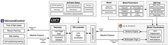
Figure 1. Architecture of the simulation framework.

All parameters are derived from a custom lift quadrotor, Buho Negro, developed by The Aeronautics and Thermofluids Applied (ATA) research group of the National Polytechnic School. Buho Negro was first modeled in CAD 2025 Sp5 and used to 3D-print selected structural parts, and avionics were integrated for flight. Parameter identification combines (i) measurements on the physical platform, (ii) CAD-based geometry and inertial properties, and (iii) manufacturer data for the ESC–motor–propeller set. Unless otherwise noted, all quantities are expressed in SI units and mapped directly to SDF fields and PX4/Gazebo plugin inputs.

2.1. UAV Gazebo Modeling

High-fidelity behavior in Gazebo requires a consistent set of inputs that represent the UAV’s geometric/visual description, sensor configuration, and propulsion dynamics. These inputs define links/joints and frames in SDF and configure PX4–Gazebo plugins for sensing and actuation. For clarity we group parameters into: (i) geometric and visual parameters, (ii) sensor configuration, and (iii) propulsion system characteristics.

2.1.1. Geometric and Physics Parameters

The geometric and physical characterization of the digital twin began with the assembly of the Búho Negro quadrotor, designed specifically for this study. The platform, configured in an “X” layout, integrates a battery, ESCs, a flight controller, a GPS module, and inertial sensors (see Figure 2a). After assembly, the total mass was measured as 5.86 kg, which was used as a reference for constructing the virtual model.

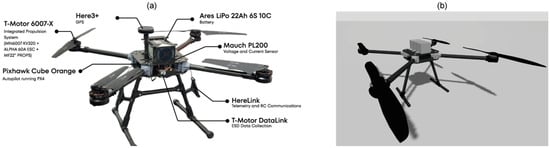
Figure 2. Buho Negro Quadrotor for the study case: (a) real quadrotor setup, (b) Gazebo Harmonic model.

A CAD model was created in Fusion 360 to faithfully reproduce the geometry and component layout. To match the total mass and its distribution, representative electronic components with adjusted densities were added. Using Fusion 360’s rigid-body analysis tools, the center of mass (CoM) was located 0.34 m above the base plane, and the principal moments of inertia were Ixx = 0.179 kg·m², Iyy = 0.180 kg·m², and Izz = 0.303 kg·m². These parameters were incorporated into the model’s SDF file using the <inertial> and <pose> tags, aligning the CoM with the origin of the simulation coordinate system.

Motor and propeller positions were extracted directly from the CAD and expressed relative to the CoM. Propeller mass was included to capture rotor inertial effects, which is essential for subsequent propulsion-system parameterization. For Gazebo visualization, the CAD was exported to STL and processed in Blender to generate a “.dae” mesh referenced by the <visual> tag (Figure 2b).

2.1.2. Propulsion System

Propulsion is simulated with the MulticopterMotorModel plugin, which models each rotor as an ESC–motor–propeller chain and computes thrust/torque from rotor speed commands [12]. To ensure correct parameterization, we inspected the plugin’s API and source [13]. In the architecture in Figure 1, the resulting parameters populate: Model Parameters (actuator time constants, rotor speed constants), the SDF File (plugin configuration and link/joint mapping), and the Airframe Setup (speed limits and control allocator). PX4 sends motor-speed references to Gazebo.

The physical chain on Búho Negro consists of a T-Motor ALPHA 60 A 6S FOC ESC [14], T-Motor MN6007-II KV320 motor [15], and 22.4 × 8 in propellers (MF2211) [16].

Actuator Dynamics (Time Constants)

The plugin is modeled as a rotor-speed tracking with a first-order response [12,13,17]

$${\displaystyle \frac{\omega \left(s\right)}{{\omega }_{ref}\left(s\right)}}={\displaystyle \frac{1}{\tau s+1}},$$

(1)

where ${\omega }_{ref}\left(s\right)$ (from PX4) is the commanded speed and $\omega \left(s\right)$ the realized speed in the Laplace space. The time constant $\tau$ differs for acceleration ${\tau }_{up}$ and braking ${\tau }_{down}$.

The ESC datasheet reports a Throttle Response Speed of 50 ms, the time required for the output to rise from 10% to 90% after a step command [14]. Interpreting this as the rise time $t_r$ of the first-order law in (1), and using the standard relation $t_r=2.2\tau$ [18], yields ${\tau }_{up}=0.023\mathrm{s}$. For braking, FOC ESCs typically require 5–20% longer than acceleration [19]; we adopt a conservative ${\tau }_{down}=1.2 s$, ${\tau }_{up}=0.028s$.

Motor Constant and Moment Constant

In the MulticopterMotorModel plugin, the thrust and aerodynamic torque generated by each rotor are computed from the rotor’s angular speed ω according to [12,13]:

$$T=k_t{\omega }^2 \left[\mathrm{N}\right]$$

(2)

$$Q=k_{m}T \left[\mathrm{Nm}\right],$$

(3)

where $T$ is the thrust produced by a single rotor and is applied along the rotor axis defined in the SDF; $Q$ is the aerodynamic drag torque about that axis, which contributes to yaw authority. The sign of $Q$ follows the rotor’s configured turning direction in the plugin. The variable ω is the rotor speed commanded by PX4’s control allocator (see Figure 1) and realized in simulation by the plugin’s first-order speed-tracking dynamics. The thrust constant $k_t\left[{\displaystyle \frac{N}{{\left(rad/s\right)}^2}}\right]$ encapsulates the combined effects of air density, propeller size, and blade geometry, while the moment constant $k_m$ [m] represents the effective ratio Q/T (a length scale).

To identify the constants, we rely on experimental data reported in [15], which provide, at different throttle setpoints, $\omega ,$ $Q$, and $T$. With measurements of $T$ and $\omega$ for the 22 × 6.6 propeller and the physical relation in (2), we rescaled the independent variable as $x={\omega }^2$ and estimated $k_t$ via ordinary least squares (OLS) regression through the origin. Similarly, $k_m$ was obtained by fitting (3) with OLS on Q as a function of T.

Figure 3 compares the OLS fits (lines) with the manufacturer’s curves (markers): (a) T vs. ${\omega }^2$ and (b) Q vs. T. In both cases, the fit nearly coincides with the manufacturer data, with coefficients of determination $R^2=0.9993$ and $R^2=0.9998$, respectively. These values indicate that more than 99.9% of the observed variation is explained by the linear models and that residuals are small within the fitted range. Consequently, the OLS slopes directly yield the actuator parameters:$k_t=1.881\times {10}^{-4}$ and $k_m=0.0238$.

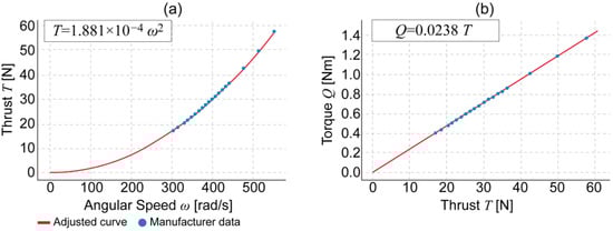
Figure 3. Identification of thrust and moment constants from manufacturer data: (a) Thrust T versus angular speed ω for the 22 × 6.6 in propeller. (b) Aerodynamic torque Q versus thrust T for the same propeller.

When detailed torque/thrust curves are unavailable for the target propeller, as in our case, where data exist for a 22 × 6.6 in propeller while the Búho Negro platform uses 22.4 × 8 in, we apply similarity-based scaling. The derivation starts from the thrust-coefficient identity [20].

$$C_T={\displaystyle \frac{T}{\rho \hspace{0.17em}{n}^2\hspace{0.17em}{D}^4}}$$

(4)

where $\rho$ is air density, $\hspace{0.17em}n$ is rotational speed in revolutions per second (if given in rpm), and $D$ is diameter. Using $\omega =2\pi n$ and (2), the thrust becomes constant:

$$k_t={\displaystyle \frac{\rho \hspace{0.17em}{C}_T}{4{\pi }^2}}{D}^4$$

(5)

Under geometric proximity (same propeller family, blade count, and comparable solidity) and a quasi-static operating regime, $C_T$ varies approximately with $P/D$, leading to the practical scaling $k_t\propto D^{3}P$ [20,21] and thus

$$k_{t2}=k_{t1}{\displaystyle \frac{{D_2}^3{P}_2}{{D_1}^3\hspace{0.17em}{P}_1}}$$

(6)

Here, $P$ is the pitch, subscript 1 refers to the 22 × 6.6 in reference propeller and subscript 2 to the 22.4 × 8 in target propeller. With $k_t=1.881\times {10}^{-4}$ for the 22 × 6.6 in propeller, the scale factor is $k_t=2.4066\times {10}^{-4}$ for the 22.4 × 8 in propeller.

For the moment constant, we retain km as a first-order approximation, setting $k_{m2}=k_{m1}=0.0238,$ since torque scales with thrust and, within our operating range, the thrust–torque ratio is not expected to vary appreciably between these closely related propellers.

Maximum Rotor Speed

The maximum rotor speed was estimated from the manufacturer’s data for the 22 × 6.6 in propeller as ${\omega }_{max1}$ = 551 rad/s. When scaling the thrust constant from $k_{t1}$ to $k_{t2}$ for the P22.4 × 8 in propeller, while maintaining the same thrust, the following condition must be satisfied:

$${\omega }_{max2}={\omega }_{max1}\cdot \sqrt{{\displaystyle \frac{k_{t1}}{k_{t2}}}}=487.$$

(7)

2.2. PX4 Airframe Configuration and Ground-Control Integration

Building the digital twin in PX4–Gazebo requires two artifacts defined in concert: (i) the SDF model and (ii) the PX4 airframe (see Figure 1), which configures actuator mapping (rotor indices and turning directions), the control allocator, controller gains, and simulation limits. In this work we started from a standard X-type template and updated rotor locations and directions to match the CAD, then tuned attitude and position gains to the target mass–inertia.

2.2.1. Command and Telemetry Path

Figure 1 shows the simulation information flow: QGroundControl sends mission plans and parameter updates to PX4, whose control allocator computes per-motor speed refs ${\omega }_{ref}$ and forwards them to Gazebo. The MulticopterMotorModel applies first-order rotor dynamics to produce thrust and reaction torque. Simulated IMU/GPS/barometer streams return to PX4 for state estimation and to QGroundControl for visualization/logging, closing the loop.

2.2.2. Rotor-Speed Limits and Saturation

Because the propulsion plugin operates with absolute angular speed in rad/s, rotor limits must be identical in the airframe and in the plugin. From Section 2.1.2 we adopt ${\omega }_{max}$= 487. Flight observations indicate rotation begins around 20% throttle and normal operation extends to 95% of maximum, so we set ${\omega }_{min}=0.20{\omega }_{max}=97.4$ and ${\omega }_{nmax}=0.95{\omega }_{max}=462.65$. These values are written in the airframe in SIM_GZ_EC_MIN and SIM_GZ_EC_MAX and mirrored in the SDF plugin.

3. Experiments and Results

Following the methodology described in Section 2, the quadrotor parameters were derived and are summarized in Table 1. All values are consistent with the physical Búho Negro platform and were cross-checked against the real vehicle’s configuration.

Table 1. Buho quadrotor physical parameters.

Parameter	Value	Parameter	Value
Total Mass without propellers (m)	5.86 Kg	Up time Constant (tr)	0.023 s
Center of mass	0, 0, 0.34 (m)	Down time Constant (td)	0.028 s
Propeller mass	0.07 kg (each)	Motor Constant (kt)	2.4066 × 10−4 N s2/rad2
Propeller location	1: 0.365 m (X) −0.365 m (Y) 0.02 m (Z) 2: −0.365 m (X) 0.365 m (Y) 0.02 m (Z) 3: 0.365 m (X) 0.365 m (Y) 0.02 m (Z) 4: −0.365 m (X) −0.365 m (Y) 0.02 m (Z)	Moment Constant (km) Maximum Motor Velocity Rolling Moment Coefficient Motor Drag Coefficient	0.0238 m 487 rad/s 1 × 10−6 1 × 10−3

To evaluate model fidelity, two autonomous missions were designed in QGroundControl (each with distinct trajectories and altitude profiles) and executed at the stadium of the Escuela Politécnica Nacional. The flight plan comprised multiple waypoints with programmed changes in altitude and orientation and was flown by both the physical drone and the simulated model. In both cases, onboard telemetry was recorded via PX4 log files for subsequent time-aligned analysis.

Figure 4 shows the simulated flights in the Gazebo environment for the two autonomous missions described earlier. The trajectories executed in simulation are identical to those performed by the physical model, each consisting of three sequential takeoff–waypoint–landing tasks. The simulated world replicates the location and visual features of the Estadio de la Escuela Politécnica Nacional (EPN) and was incorporated into Gazebo for the simulation, as introduced in Figure 1.

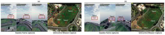
Figure 4. Gazebo mission results: (a) Mission 1 frames, (b) Mission 2 frames.

The left sequence corresponds to Mission 1, in which the UAV follows a triangular pattern with three widely spaced takeoff points at a constant altitude of 50 m. This mission aims to verify the correct execution of both trajectory and altitude tracking. Due to its simplicity, most of the flight time is spent cruising in straight-line segments between takeoff points.

In contrast, the right sequence corresponds to Mission 2, which follows a denser pattern with shorter inter-point distances and multiple turns, forming a grid-like trajectory. This mission places greater maneuvering demands on the UAV, with altitude varying between 50 m and 100 m and sharp turns at Take 2 and Take 3. The goal is to visually assess the model’s behavior under more dynamic flight conditions.

Both missions were executed by the simulated and physical platforms, with onboard telemetry (PX4 logs) recorded in each case for subsequent time-aligned comparison.

After completing the flight missions, a comparative analysis of the telemetry data was conducted. The key metrics focused on four variables: XY-plane trajectory, altitude (Z), total throttle signal and per-motor PWM.

Figure 5 and Figure 6a compare the normalized PWM values sent to each of the four motors during the mission. While both the simulated and real curves follow a common trend, notable differences in magnitude and variability are observed. The real signals exhibit more noise and spread, which is expected due to aerodynamic disturbances, propeller imbalance, and nonlinear behavior of the physical system. In contrast, the simulated model shows cleaner transitions and discrete steps, reflecting the idealized behavior of the MulticopterMotorModel plugin. The most significant discrepancies occur during yaw maneuvers, suggesting that the current model does not sufficiently capture the dynamic effects of rapid directional changes.

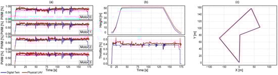
Figure 5. Mission 1 comparison results: (a) PWM signals, (b) height and throttle, (c) trajectory.

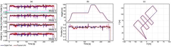
Figure 6. Mission 2 comparison results: (a) PWM signals, (b) height and throttle, (c) trajectory.

Figure 5 and Figure 6b show the comparison between estimated altitude (Z) and throttle commands (%) over the mission duration. Both signals exhibit an overall agreement between simulation and real flight, with a steep initial ascent, a steady cruising phase near the top, and a controlled descent. Meanwhile, the simulated throttle signal appears smoother than the real one, with slight oscillations during regime transitions. This difference is attributed to the absence of wind modeling and simplified ESC dynamics in the simulated model.

Figure 5 and Figure 6c illustrate the projected horizontal XY trajectory. Like the altitude result, this value falls within the typical accuracy range of civilian-grade GPS receivers (2–10 m horizontally). Finally, Table 2 indicates higher fidelity under nominal conditions (Mission 1) and greater variability under maneuvering demands (Mission 2). In Mission 1, errors are lower and more tightly distributed for trajectory (RMSE 3.350 m; P75 4.488 m) and altitude (RMSE 2.291 m; P75 2.298 m), consistent with the triangular path and constant altitude. In Mission 2, the grid-like pattern with tight turns and altitude changes increases dispersion (trajectory P75 6.155 m; altitude P75 3.291 m). Motor outputs also exhibit substantially higher variation (P75 11.2% vs. 1.2% in Mission 1). Although throttle errors remain modest on average (RMSE 5.2%, median 1.5%), rapid maneuvers and altitude transitions induce larger, uneven corrections across motors, amplifying departures from the physical system. Overall, the model is validated in nominal regimes and calls for targeted refinements for fast, highly dynamic maneuvers.

Table 2. Error metrics.

	Mission 1				Mission 2
Metric	Trajectory (m)	Height (m)	Throttle (%)	Motor Outputs (%)	Trajectory (m)	Height (m)	Throttle (%)	Motor Outputs (%)
RMSE	3.350	2.291	6.7	13.5	4.435	3.156	5.2	12.3
Median	2.709	1.777	3.0	8.5	2.477	2.519	1.5	7.5
25th percentile	0.732	1.719	2.2	5.2	2.140	2.428	0.7	4.3
75th percentile	4.488	2.298	4.2	1.2	6.155	3.291	2.7	11.2

4. Conclusions

The results show that the quadrotor simulation scheme, built using the parameters defined in Section 2.1 and without external disturbance models, provides a reasonably accurate representation of the real system’s dynamic behavior. Altitude and trajectory alignment are strong, and the deviations fall within the accuracy thresholds of the sensors used. The differences observed in motor response and attitude commands can be explained by the absence of a wind model, as well as the lack of detailed representation of phenomena such as wiring losses, inertia variations, or mechanical friction. Furthermore, the physical system’s dynamics include delays, hysteresis, and saturation effects that are not present in the idealized simulation environment.

The most significant discrepancies are concentrated in two key aspects. First, the lower variability of the simulated signals can be attributed to the absence of wind and other stochastic effects present in the physical environment. Second, the oscillations observed in the attitude angles during aggressive maneuvers are not accurately replicated in the simulation, suggesting a need to refine the rotational dynamics model.

References

- Spencer, D. Industry Analysis: Unmanned Aerial Systems. Muma Bus. Rev. 2018, 2, 83–104. [Google Scholar] [CrossRef] [PubMed]
- Piljek, P.; Kotarski, D.; Krznar, M. Method for Characterization of a Multirotor UAV Electric Propulsion System. Appl. Sci. 2020, 10, 8229. [Google Scholar] [CrossRef]
- Valencia, E.; Changoluisa, I.; Palma, K.; Cruz, P.; Ayala, P. Wetland Monitoring Technification for the Ecuadorian Andean Region Based on a Multi-Agent Framework. Heliyon 2022, 8, e09054. [Google Scholar] [CrossRef] [PubMed]
- Manfreda, S.; McCabe, M.; Miller, P.; Lucas, R.; Pajuelo, V. On the Use of Unmanned Aerial Systems for Environmental Monitoring. Remote Sens. 2018, 10, 641. [Google Scholar] [CrossRef]
- Aláez, D.; Olaz, X.; Prieto, M.; Villadangos, J.; Astrain, J.J. VTOL UAV Digital Twin for Take-Off, Hovering and Landing in Different Wind Conditions. Simul. Model. Pract. Theory 2023, 123, 102703. [Google Scholar] [CrossRef]
- Tullu, A.; Jung, S.; Lee, S.; Ko, S. Effects of Model-Specific Parameters on the Development of Custom Module in PX4 Autopilot Software-in-the-Loop. Int. J. Aerosp. Eng. 2025, 2025, 4886534. [Google Scholar] [CrossRef]
- García, J.; Molina, J.M. Simulation in Real Conditions of Navigation and Obstacle Avoidance with PX4/Gazebo Platform. Pers. Ubiquitous Comput. 2022, 26, 1171–1191. [Google Scholar] [CrossRef]
- Xu, X.; Sun, J.; Hu, H. Simulator-Based Mission Optimization for Swarm UAVs with Minimum Safety Distance Between Neighbors. In Proceedings of the AIAA AVIATION 2023 Forum, San Diego, CA, USA, 12–16 June 2023; p. 4453. [Google Scholar]
- PX4 Documentation. Gazebo Simulation|PX4 User Guide (v1.12). 2025. Available online: https://docs.px4.io/v1.12/en/simulation/gazebo.html (accessed on 22 July 2025).
- TSC21. Documentation: What is the Math Behind the Motor Model? July 2017. Available online: https://github.com/PX4/PX4-SITL_gazebo-classic/issues/110 (accessed on 22 July 2025).
- Mairaj, A.; Baba, A.I.; Javaid, A.Y. Application-Specific Drone Simulators: Recent Advances and Challenges. Simul. Model. Pract. Theory 2019, 94, 100–117. [Google Scholar] [CrossRef]
- Open Source Robotics Foundation. Class Ignition::Gazebo::Systems::MulticopterMotorModel. Gazebo 6.17.0 API Documentation. 2025. Available online: https://gazebosim.org/api/gazebo/6/classignition_1_1gazebo_1_1systems_1_1MulticopterMotorModel.html (accessed on 2 August 2025).
- GazeboSim. MulticopterMotorModel.cc; Gz-sim Repository, Commit 72211093a85ff91cddf9350628d870c3dbbdf635, Lines 261–284. 2025. Available online: https://github.com/gazebosim/gz-sim/blob/72211093a85ff91cddf9350628d870c3dbbdf635/src/systems/multicopter_motor_model/MulticopterMotorModel.cc#L261-L284 (accessed on 2 August 2025).
- T-MOTOR. Alpha 60A 6S ESC. 2025. Available online: https://store.tmotor.com/product/alpha-60a-6s-esc.html (accessed on 2 August 2025).
- T-MOTOR. MN6007 V2 Motor (Antigravity Type). 2025. Available online: https://store.tmotor.com/product/mn6007-v2-motor-antigravity-type.html (accessed on 2 August 2025).
- T-MOTOR. Polymer Folding Propeller 08×15. 2018. Available online: https://uav-en.tmotor.com/2018/Polymer_Folding_0815/178.html (accessed on 2 August 2025).
- ROS.org. Class FirstOrderFilter. Rotors_gazebo_plugins ROS Melodic API Documentation. Available online: https://docs.ros.org/en/melodic/api/rotors_gazebo_plugins/html/classFirstOrderFilter.html#details (accessed on 2 August 2025).
- Nise, N.S. Control Systems Engineering, 7th ed.; Wiley: Hoboken, NJ, USA, 2015. [Google Scholar]
- Texas Instruments. High-Speed Sensorless-FOC Reference Design for Drone ESCs (TIDA-00916). Dec. 2016. Available online: https://www.ti.com/lit/pdf/tiducf1 (accessed on 1 August 2025).
- Brandt, J.B.; Selig, M.S. Propeller Performance Data at Low Reynolds Numbers. In Proceedings of the 49th AIAA Aerospace Sciences Meeting, Orlando, FL, USA, 4–7 January 2011; American Institute of Aeronautics and Astronautics: Reston, VA, USA, January 2011. [Google Scholar] [CrossRef]
- Brezina, A.J.; Thomas, S.K. Measurement of Static and Dynamic Performance Characteristics of Electric Propulsion Systems. In Proceedings of the 51st AIAA Aerospace Sciences Meeting including the New Horizons Forum and Aerospace Exposition, Grapevine, TX, USA, 7–10 January 2013; American Institute of Aeronautics and Astronautics: Reston, VA, USA, January 2013. [Google Scholar] [CrossRef]
Disclaimer/Publisher’s Note: The statements, opinions and data contained in all publications are solely those of the individual author(s) and contributor(s) and not of MDPI and/or the editor(s). MDPI and/or the editor(s) disclaim responsibility for any injury to people or property resulting from any ideas, methods, instructions or products referred to in the content. |
© 2025 by the authors. Licensee MDPI, Basel, Switzerland. This article is an open access article distributed under the terms and conditions of the Creative Commons Attribution (CC BY) license (https://creativecommons.org/licenses/by/4.0/).