Comparative Analysis of Stress Serration Characteristics in AlMg3 Alloys ^†

Abstract

Aluminum–magnesium alloys show the Portevin–Le Chatelier (PLC) effect. The aim of this publication is to provide a detailed analysis of the evaluation methods of this phenomenon using tensile tests at a strain rate range of 10⁻³ s⁻¹, where A and A + B stress serrations can be observed. Four smoothing and analytical functions are evaluated in detail as reference functions, which are compared based on their serration amplitude and frequency characteristics. The studied functions are the moving average and Savitzky–Golay smoothing method, as well as the Voce and polynomial analytic functions. The two smoothing methods and smoothing window sizes are compared to obtain the best reference function parameters.

1. Introduction

The stress serrations observed during tensile testing were first published by Portevin and Le Chatelier [1]; this is why this phenomenon is uniformly called the PLC effect in the literature. The three basic types of stress serrations are distinguished by the letters A, B, and C. Their shape is introduced in several publications; a comprehensive overview of them can be found in the review paper by Zhang et al. [2]. The main characteristic of the PLC effect is the stress serration amplitude obtained from the tensile test curve. The parameters of this have been defined by several authors, such as, among others, Saad et al. and Tian et al. [3,4]. The differences between the positive and negative peaks of the tensile test curve give the amplitudes of the stress serrations (Δσ). In addition to direct measurements, another evaluation is widespread which uses a so-called reference function calculated from the stress–strain or stress-time curves using appropriate smoothing. In this case, the difference between the measured stress and the reference function gives the amplitude of the stress serrations. This function oscillates around zero, which allows for further analysis, primarily for using Fast Fourier Transform (FFT); an example of this analysis can be found in the work of Yuan et al. [5]. The application of the reference function already appears in early evaluations, for example, in the work of Lebyodkin et al. [6], who calculated the amplitude of the stress serrations from straight reference lines fitted to the stress–strain curve step by step. In the papers by Saad et al. [3] and Bakare et al. [7], the deviation from Hollomon’s power function was considered. A formal mathematical approximation was offered in the form of a ninth-degree polynomial by Lebyodkin et al. [8]. Various curve-smoothing procedures have also been used as reference functions, such as the moving average approximation [9] and the Savitzky–Golay polynomial smoothing method [10]. A mathematical model was presented by Savitzky et al. [11]; a possible application and computational example can be found in the work of Guiñón et al. [12]. Using these smoothing functions, adequate approximations of stress serrations can be obtained, but the number of measurement points included in the smoothing window must be determined with care.

The amplitude of stress serrations alone characterizes the PLC effect, but several authors propose a dimensionless normalized form, which can be calculated by the relative value of Δσ/σ [6,7,9,10]. For the statistical analysis of stress serrations, the review works of Lebyodkin et al. [8,13] provide important information. The probability density function of stress amplitudes can also be related to the type of serration, an example of which is presented in the paper by Chatterjee et al. [14]. An important note is included in the work by Lebyodkin et al. [15], which states, in agreement with other authors, that small serration amplitudes close to 0 can arise from the noise of force measurement, and additional small stress serrations, which gradually increase with increasing strain, can also occur because of plastic deformation independently of the PLC effect. Therefore, it is quite difficult to distinguish them from B-type serrations. Stress–time functions are mainly used for these analyses, as their data series is equally spaced and the distance between the measurement points is determined by the sampling frequency, which is typically 50–100 Hz in strain rates in the range of 10⁻³–10⁻⁵ s⁻¹. A higher frequency is also recommended for strain rates of 10⁻² s⁻¹. The stress values obtained from tensile tests are classified as engineering stress in some publications, while true stress is used in others.

From the presented literature review, it can be stated that there is no uniform measurement method for characterizing the amplitude of stress serrations; several evaluation models are used in the literature. Therefore, it seems expedient to carry out a comparative analysis of the individual solutions to clarify how the magnitude of the parameters derived from the measurement results is affected by the choice of evaluation method. For analysis of stress serrations, the AlMg3 aluminum alloy was selected. Samples were examined in a strain rate range of 10⁻³ s⁻¹, where type A and B serration patterns appeared on the tensile diagrams. By fitting four reference functions to the measured curves, the effect of each function on the amplitude of PLC stress serrations and the amplitude-frequency function of fast Fourier transform (FFT) have been studied.

2. Materials and Methods

The tested AlMg3 sheet was delivered in a hardness grade of H22. Its thickness was 2.5 mm; the main alloying elements of the sheet were Mg 3.5%, Si 0.06%, Fe 0.14%, Mn 0.36%, and Cu 0.002%. The tensile test characteristics of the as-received sheet were the following: yield strength 156 MPa, ultimate tensile strength 256 MPa, uniform elongation 14.7%, elongation at fracture 19.2%, hardening exponent 0.26, and plastic anisotropy 0.63.

The tensile tests were performed using a 100 kN capacity Instron^® 5582 tensile testing machine (Norwood, MA, USA) with a video extensometer strain measurement device. The extensometer measured the longitudinal and the transverse strains between two points. The gauge length of the specimens was 80 mm, the cross-section area was 20 mm × 2.5 mm, and the strain rate was 5 × 10⁻³ s⁻¹; the specimens were cut parallel to the rolling direction. The test results were recorded using a 50 Hz sampling frequency and were evaluated using the Instron’s Bluehill2 software. Further calculations were made using MS Excel and Origin 9.0 software.

Related to the evaluation of serrations, this paper uses a so-called reference function calculated from the engineering stress–time curve points. The difference between the measured stress and the reference function gives the amplitude of the stress serrations. Four reference functions are used: Moving Average (MA), Savitzky–Golay smoothing (SG), four-parameter Voce function (V4), and ninth-degree polynomial (P9). The analytical functions can be characterized by the equations below in the engineering stress–time coordinate system.

Voce function:

$${\sigma }_{eng}=a+b\left(1-exp\left(-c{t}^d\right)\right)$$

(1)

Polynomial function:

$${\sigma }_{eng}=a_0+{\sum }_{i=1}^9{a}_i{t}_i^i$$

(2)

where a, b, c, and d are material constants in Equation (1), and a₀ and a_i are coefficients of the polynomial equation.

3. Results and Discussion

The tensile test curves of the tested AlMg3 sheets show serrations of type A and A + B in strain rates in the range of 10⁻³ s⁻¹. As a starting point, it is useful to consider Figure 1a, which shows two highlighted details of the engineering stress–time curve. At the beginning of the curve, type A serrations can be observed (for example, at 13 s, there is 5.8% axial strain; see the left magnified window), which change from ~18 s (~9% strain) to A + B type, with characteristic B-type sections. Figure 1b shows the approximation of smaller-amplitude serrations (red line) following a higher stress drop, with a reference function (green line) and the amplitude interpretation of the Δσ stress serration from the upper peak to the lower valley. At the same time, the deviations from the upper and lower peaks to the reference function are Δσ₁ and Δσ₂; the sum of them does not equal the value of Δσ. Therefore, a detailed investigation is necessary to determine how the different analyses based on deviations from the reference function differ from each other.

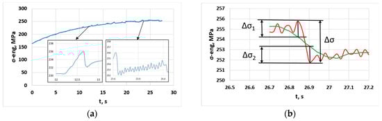
Figure 1. Details of tensile test curve and serration amplitudes: (a) parts of tensile test curve; (b) interpretation of serration amplitudes.

Based on the literature survey, it was established that stress serrations can be mainly determined in the form of deviations from the reference function. In the following sub-sections, the kinds and parameterizations of the reference functions will be analyzed in detail.

3.1. Analysis of Parameterization of Smoothing Functions

3.1.1. Approximation Abilities of Smoothing Functions

The moving average approximation (MA) recommended by Bharathi et al. [9] or the Savitzky–Golay polynomial smoothing (SG) method applied by Lee et al. [10] can only be used if the window of the smoothing function has been carefully determined. Figure 2 shows the effect that the number of window points (e.g., SG9: nine points in the window selected for smoothing) has on the shape of the reference functions. In both figures, the original engineering stress–time diagram is shown with a thick line, and the approximation with the Savitzky–Golay quadratic polynomials are illustrated by thinner lines. In Figure 2b, the 9-point smoothing window gives the closest fit, while the original tensile test curve and the 33-point smoothing results show the least accurate curve. As a result, the values Δσ₁ and Δσ₂, calculated from the smoothing function SG9, will be significantly smaller than the values obtained from the 33-point window. The analytical reference function (V4), defined by the four-parameter Voce function with Equation (1), can also be seen here, which is fitted to the tensile test curve and approximates the stress–time function in the examined sections globally. The type A (Figure 2a) and A + B (Figure 2b) serrations are approximated in different ways compared to the smoothing functions. These differences influence the measured frequency of serrations. However, the V4 hardening model only shows the global trend of tensile test data; it does not follow the serration pattern details in Figure 2b.

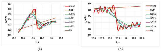
Figure 2. Effect of window size on the shape of reference functions: (a) approximation of type A serration; (b) approximation of A + B type serrations.

From the examples presented, when choosing the smoothing parameters, for the correct evaluation of amplitude and frequency, the parameters should be optimized, but it is also obvious that the two parameters cannot be satisfied with the same window size perfectly. The position of the Voce reference function presented as an example indicates that the fitting made to the entire tensile test curve with analytic functions follows the local changes in the curve, with significant differences.

Figure 3a shows the effect of the size of the window on the stress amplitude Δσ, and Figure 3b shows the effect of the window size on the amplitude–frequency function of FFT derived from the stress amplitude–time function. In Figure 3a, the maximum amplitudes calculated from the Δσ-9 function remain below 1 MPa, but the SG33 window size results peaks above 2 MPa. The window size on the FFT amplitude–frequency function is even more illustrative (see Figure 3b): here, the first peak of SG33 smoothing occurs at a frequency of around 2 Hz, then the decreasing window size results in a smaller amplitude and a shift in the first peak to higher frequencies. In contrast, the second peaks, characteristic of type B serrations, appear around 20 Hz, with almost the same amplitude.

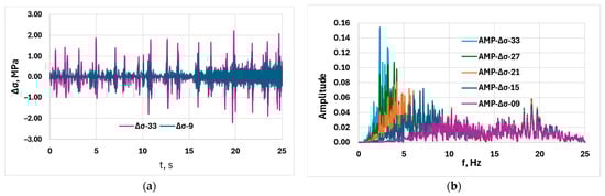
Figure 3. Effect of window size (a) on serration amplitudes and (b) on FFT functions.

3.1.2. The Effect of Window Size on the Numerical Characteristics of Serrations

The examples presented above support the conclusion that the type and parameters of the reference function have a significant influence on the value of the derived quantities, namely, the engineering stress amplitude–time function and its Fast Fourier Transform. Therefore, the numerical data and conclusions drawn from them are only valid with the given parameterization. Due to the significant differences, the question arises of whether there is an “optimal” reference function for the evaluation of the examined type A and B serrations.

The determination of the size of the compromise window is aided by the two diagrams in Figure 4. The blue function in Figure 4a illustrates the difference between the average of the ten positive and ten negative peaks of the engineering stress amplitude Δσ-10-ave, illustrated in Figure 3a for the tested window sizes (SG9-SG33), which shows a clear upward trend alongside the increase in window size. The orange function shows the frequency of the serrations, or, by definition, the change in the average number of serrations during the test (total serrations/test duration). As the diagrams in Figure 2 illustrate, the reference function determined by the largest window (SG33) returns to the serrations of the tensile test curve at the latest, so, obviously, the number of serrations calculated from it will be the smallest. Figure 4b quantifies the FFT functions shown in Figure 3b, where the first amplitude peak and its frequency are indicated. Both figures clearly prove that amplitude and frequency functions show opposite changes depending on the window size, so they can only be determined at the same time at the cost of a compromise in the manner described. As a comparative analysis of the examined SG9–SG33 ranges, the reference function, which was calculated using 21 window points, seemed to be the most favorable for the analysis of the given tensile test curves, so, in further evaluations, the 21-point window size of SG and MA smoothing are mostly used. At the same time, the results of the two extreme values can be used in different ways. If the evaluation of the amplitude is the most important aspect, it is advisable to use a higher window size, but if the emphasis is on frequency analysis, then a narrower window should be considered.

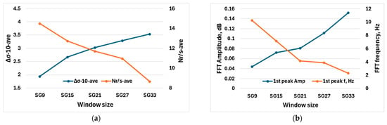
Figure 4. Effect of window size: (a) serration amplitude and average number of serrations; (b) FFT amplitude and frequency.

Of course, the studies also covered the reference function calculated from the moving average. In this case, the approximation also strongly depends on the chosen window size, and, to be comparable with the Saviczky-Golay smoothing, a 21-point window was also used. The tests showed that the Savitzky–Golay smoothing follows the engineering stress–time function more accurately than the reference function calculated from the moving average. Figure 5a,b shows the Short-Time Fourier Transform (STFT) values for the MA and SG data. It is obvious that there is a significant difference between the SG and MA charts. The MA peaks are higher, but the lower-frequency band is smaller (0–5 Hz) and the larger-frequency band is around 20 s is narrower. Taken together, this representation shows the differences between the two types of smoothing functions in the representation of the Δσ peaks and FFT spectrum.

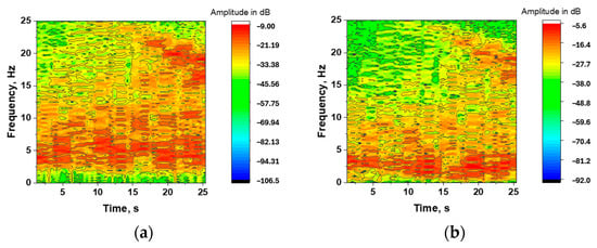
Figure 5. Comparison of Savitzky–Golay and moving average smoothing: (a) STFT chart (SG21); (b) STFT chart (MA21).

3.2. Analysis of the Serrations Derived from the Analytic Reference Functions

The stress amplitudes calculated from the Voce analytic function (V4) and the 9-degree polynomial approximation (P9) are illustrated in Figure 6. The analytic functions follow the engineering stress–time curve globally, so the calculated differences between the measured values and the reference functions are significantly larger than in case of the previously presented smoothing reference function approximation. It can also be observed that some details of the Δσ serrations obtained from the V4 and P9 do not fluctuate locally around stress 0, but differ significantly from it, while the results of the MA and SG smoothing give a nearly symmetrical amplitude distribution to the 0-axis, but, compared to the analytic function approximation, the amplitude peaks are 2–2.5 times smaller.

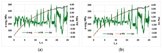
Figure 6. Comparison of serration amplitudes: (a) Voce approximation; (b) polynomial approximation.

3.3. Comparative Analysis of the Four Selected Reference Functions

In this sub-section, the four selected reference functions are compared. Figure 7 illustrates that the polynomial (P9) and the Voce (V4) approximations only follow the engineering test curve globally, while the MA and SG reference functions follow locally. Figure 7a primarily illustrates the approximation of type A serrations with the reference function, while Figure 7b shows the tracing of type A + B serrations. From the comparison of the two figures, in the 10–15 s time ranges (~4.3–7.3% elongation), type A serrations are better characterized by analytical reference functions, as they show the deviation from the general stress level more accurately. On the other hand, A + B serrations at 20–25 s time ranges (~10–13% elongation) are more appropriately followed by smoothing functions.

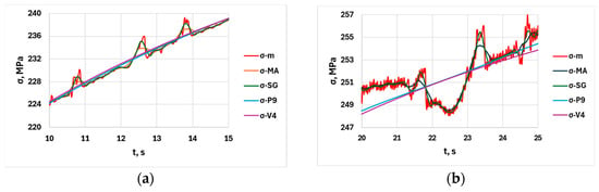
Figure 7. Comparison of reference functions: (a) A-type serrations (ε_ave ≈ 5.8%); (b) A + B type serrations (ε_ave ≈ 11.5%).

The comparison of the Δσ–time functions calculated from the five window sizes and the analytical reference functions V4 and P9 are analyzed together using the correlation coefficient matrix, partly illustrated in Figure 8. The only objective of this study is to estimate the similarity or dissimilarity of these functions. Figure 8a shows the magnitude of all correlation coefficients relative to the reference function SG9. The emphasis on SG9 is justified because it is the one that best follows the tensile test curve among the approximations. From the chart, it can be seen that, as the window size (W) increases, the correlation coefficient decreases, so the smoothing function approaches the measured stress less. Furthermore, the correlation coefficients of MA are consistently smaller than the SG values. The last two columns show the correlation coefficients (AN) of the analytic functions: here, the blue column refers to V4, and the orange column refers to P9. Analytic functions approximate SG9 values to a much lesser extent than the MA and SG functions; among them, P9 gives a slightly more accurate approximation. This diagram also explains the reality of the comparisons presented above. Figure 8b shows the cross-correlation coefficients of the same calculation; in the case of SG and MA, for example, the W9-W15 indication refers to the value of the correlation coefficient between each them obtained using a 9- and 15-point window. The successive windows were approaching an upper limit; therefore, there was no reason to further increase the window size above 33 points in the present study. The rightmost two pairs of columns show the relationship between the approximations V4 and P9 with the reference functions SG21 and MA21, from which both analytic functions show greater similarity to the approximation MA.

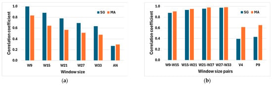
Figure 8. Correlation coefficients of different stress–time curves. (a) Coefficients related toSG9. (b) Mutual correlation coefficients.

Considering Figure 4 and Figure 8, it is obvious that the stress amplitudes calculated from the reference functions are strongly dependent on the window size of the smoothing functions. Between the analyzed SG9 and SG33 window sizes, the difference in calculated stress amplitudes is about 40%, and the frequency characteristics show even more significant differences. It follows from the above statements that, in analyses of this type of serration pattern, the selection and parameterization of the reference functions play a significant role in the research of the PLC effect. At the same time, although the evaluations based on the reference functions have significant advantages, a direct evaluation of tensile test data will offer more exact results concerning stress amplitudes.

4. Summary

During this research, the serrations appearing in the tensile test curve of an AlMg3 alloy showing the PLC effect were analyzed. The different reference functions were compared based on their serration amplitude and frequency characteristics. Special attention was paid to the moving average and Savitzky–Golay smoothing, together with the analytic functions. The main findings are as follows:

• In case of the moving average and Savitzky–Golay smoothing, the change in window size significantly affected the evaluated amplitude and frequency of the stress serrations, which are interpreted as the difference between the measured data and the reference function.
• A small window size shows the frequency properties with an adequate approximation, but significantly reduces the evaluated amplitude peaks, while larger windows show the amplitudes more accurately, but distort the frequency properties.
• If the amplitude properties are more important for a test, it is advisable to choose a larger test window, but a smaller window is more favorable for frequency analysis.
• Because of conflicting requirements, it is advisable to select the optimal size of the window in the middle of the range if both parameters need to be taken into consideration at the same time.
• The analytical approximation functions Voce4 and Polynom9 are fitted to the whole domain, so they do not follow significant engineering stress changes. For this reason, the derived serration amplitude–time functions are less suitable for further FFT or other statistical analyses.
• The comparison of serration amplitude functions using the correlation coefficient matrix showed that, compared to the 9-point Savitzky–Golay smoothing window size, the SG approximation more accurately follows the engineering stress curve than the moving average, and the two analytic functions are less favorable as reference functions.
• The stress amplitudes calculated from the reference functions are strongly dependent on the window size of the smoothing functions. Between the analyzed SG9 and SG33 window sizes, the difference in the calculated stress amplitude is about 40%, and frequency characteristics show even more significant differences.

Based on the conclusions above, in a case of an analysis in which the use of a reference function is justified for the study of the PLC effect, the optimal parameters should be determined by an examination such as the one presented here.

References

- Portevin, A.; Le Chatelier, F. On a phenomenon observed during the tensile testing of alloys undergoing transformation. C. R. Acad. Sci. Paris 1923, 176, 507–510. (In French) [Google Scholar]
- Zhang, Y.; Liu, J.P.; Chen, S.Y.; Xie, X.; Liaw, P.K.; Dahmen, K.A.; Qiao, J.W.; Wang, Y.L. Serration and noise behaviors in materials. Prog. Mater. Sci. 2017, 90, 358–460. [Google Scholar] [CrossRef]
- Saad, G.; Fayek, S.A.; Fawzy, A.; Soliman, H.N.; Nassr, E. Serrated flow and work hardening characteristics of Al-5356 alloy. J. Alloys Compd. 2010, 502, 139–146. [Google Scholar] [CrossRef]
- Tian, N.; Wang, G.; Zhou, Y.; Liu, K.; Zhao, G.; Zuo, L. Study of the Portevin–Le Chatelier (PLC) characteristics of a 5083 aluminum alloy sheet in two heat treatment states. Materials 2018, 11, 1533. [Google Scholar] [CrossRef] [PubMed]
- Yuan, Z.; Li, F.; He, M. Fast Fourier transform on analysis of Portevin–Le Chatelier effect in Al 5052. Mater. Sci. Eng. A 2011, 530, 389–395. [Google Scholar] [CrossRef]
- Lebyodkin, M.; Brechet, Y.; Estrin, Y.; Kubin, L. Statistical behaviour and strain localization patterns in the Portevin–Le Chatelier effect. Acta Mater. 1996, 44, 4531–4541. [Google Scholar] [CrossRef]
- Bakare, F.; Schieren, L.; Rouxel, B.; Jiang, L.; Langan, T.; Kupke, A.; Weiss, M.; Dorin, T. The impact of L12 dispersoids and strain rate on the Portevin–Le Chatelier effect and mechanical properties of Al–Mg alloys. Mater. Sci. Eng. A 2021, 811, 141040. [Google Scholar] [CrossRef]
- Lebyodkin, M.A.; Lebedkina, T.A.; Jacques, A. Multifractal Analysis of Unstable Plastic Flow; Nova Science Publishers, Inc.: New York, NY, USA, 2009. [Google Scholar]
- Bharathi, M.S.; Lebyodkin, M.; Ananthakrishna, G.; Fressengeas, C.; Kubin, L.P. The hidden order behind jerky flow. Acta Mater. 2002, 50, 2813–2824. [Google Scholar] [CrossRef]
- Lee, S.Y.; Chettri, S.; Sarmah, R.; Takushima, C.; Hamada, J.; Nakada, N. Serrated flow accompanied with dynamic type transition of the Portevin–Le Chatelier effect in austenitic stainless steel. J. Mater. Sci. Technol. 2023, 133, 154–164. [Google Scholar] [CrossRef]
- Savitzky, A.; Golay, M.J.E. Smoothing and differentiation of data by simplified least squares procedures. Anal. Chem. 1964, 36, 1627–1639. [Google Scholar] [CrossRef]
- Guiñón, J.L.; Ortega, E.; García-Antón, J.; Pérez-Herranz, V. Moving average and Savitzky–Golay smoothing filters using Mathcad. In Proceedings of the International Conference on Engineering Education—ICEE 2007, Coimbra, Portugal, 3–7 September 2007. [Google Scholar]
- Lebyodkin, M.A.; Lebedkina, T.A. The Portevin–Le Chatelier Effect and Beyond. In High-Entropy Materials: Theory, Experiments, and Applications; Brechtl, J., Liaw, P.K., Eds.; Springer: Cham, Switzerland, 2021; ISBN 978-3-030-77640-4. [Google Scholar]
- Chatterjee, A.; Sarkar, A.; Barat, P.; Mukherjee, P.; Gayathri, N. Character of the deformation bands in the (A + B) regime of the Portevin–Le Chatelier effect in Al–2.5%Mg alloy. Mater. Sci. Eng. A 2009, 508, 156–160. [Google Scholar] [CrossRef]
- Lebyodkin, M.A.; Kobelev, N.P.; Bougherira, Y.; Entemeyer, D.; Fressengeas, C.; Gornakov, V.S.; Lebedkina, T.A.; Shashkov, I.V. On the similarity of plastic flow processes during smooth and jerky flow: Statistical analysis. Acta Mater. 2012, 60, 3729–3740. [Google Scholar] [CrossRef]
Disclaimer/Publisher’s Note: The statements, opinions and data contained in all publications are solely those of the individual author(s) and contributor(s) and not of MDPI and/or the editor(s). MDPI and/or the editor(s) disclaim responsibility for any injury to people or property resulting from any ideas, methods, instructions or products referred to in the content. |
© 2025 by the authors. Licensee MDPI, Basel, Switzerland. This article is an open access article distributed under the terms and conditions of the Creative Commons Attribution (CC BY) license (https://creativecommons.org/licenses/by/4.0/).