Abstract
Accurate prediction of ship fuel consumption is essential for improving energy efficiency, optimizing mission planning, and ensuring operational integrity at sea. However, during complex tasks such as high-speed maneuvers, fuel consumption exhibits complex dynamics characterized by the coexistence of baseline drift and transient peaks that conventional models often fail to capture accurately, particularly the abrupt peaks. In this study, a hybrid prediction model, DGM-SVR, is presented, combining a rolling dynamic grey model (DGM (1,1)) with support vector regression (SVR). The DGM (1,1) adapts to the dynamic fuel consumption baseline and trends via a rolling window mechanism, while the SVR learns and predicts the residual sequence generated by the DGM, specifically addressing the high-amplitude fuel spikes triggered by maneuvers. Validated on a simulated dataset reflecting typical fuel spike characteristics during high-speed maneuvers, the DGM-SVR model demonstrated superior overall prediction accuracy (MAPE and RMSE) compared to standalone DGM (1,1), moving average (MA), and SVR models. Notably, DGM-SVR reduced the test set’s MAPE and RMSE by approximately 21% and 34%, respectively, relative to the next-best DGM model, and significantly improved the predictive accuracy, magnitude, and responsiveness in predicting fuel consumption spikes. The findings indicate that the DGM-SVR hybrid strategy effectively fuses DGM’s trend-fitting strength with SVR’s proficiency in capturing spikes from the residual sequence, offering a more reliable and precise method for dynamic ship fuel consumption forecasting, with considerable potential for ship energy efficiency management and intelligent operational support. This study lays a foundation for future validation on real-world operational data.
1. Introduction
Against the backdrop of global economic integration and the increasing importance of safeguarding national maritime interests, ships, as critical assets for maritime transport, resource exploitation, and military power, have seen their energy efficiency and endurance capabilities garner unprecedented attention. Fuel consumption is a core element of ship operational costs and logistical support. Particularly for naval vessels undertaking long-range missions and maintaining strategic presence, the precise prediction of fuel consumption patterns is of paramount strategic and economic value for enhancing combat effectiveness, optimizing mission planning, and ensuring sustained deployment capabilities [1]. The fuel consumption process of a ship is a complex dynamic system strongly influenced by multiple factors, including speed, load, sea conditions, maneuvering actions, and the state of the hull and propulsion systems [2], rendering its accurate prediction a challenging task.
Throughout a ship’s lifecycle and mission execution, fuel assurance is consistently central [3]. For naval applications, fuel is not only the power source for propulsion but also the fundamental enabler for maintaining combat readiness, achieving strategic mobility, and accomplishing diverse military tasks. However, the modern naval warfare environment is complex and volatile, imposing higher demands on ship maneuverability, rapid response, and sustained operational capacity. An inherent contradiction exists between the limited onboard fuel capacity of ships and the vast operational maritime areas, coupled with extended replenishment cycles. Inaccurate fuel consumption predictions can lead to flawed mission planning, misjudged endurance, and, in critical moments, loss of operational capability or perilous situations due to fuel exhaustion. Consequently, effectively addressing the challenges of fuel assurance through precise prediction and refined management is a critical issue in the development of modern naval logistical support systems, directly impacting ship readiness and strategic deterrence [4].
Particularly, in specific operational or training scenarios, ships frequently need to execute high-speed maneuvers, such as emergency evasions, tactical positioning, rapid pursuits, or interceptions [5]. These high-speed maneuvers—typically involving rapid acceleration, sustained high-speed cruising, and potentially sharp turns and decelerations—induce an instantaneous surge in the load on the ship’s power system [6]. This, in turn, triggers significant, abrupt increases, hereafter referred to as transient fuel consumption spikes or simply fuel spikes, in fuel consumption within a short period [7]. These fuel spikes cause consumption levels to far exceed those observed during steady-state navigation, and their magnitude and duration are difficult to estimate using conventional experience or simple models. Accurate prediction of these fuel consumption spikes during high-speed maneuvers is of immense military significance for commanders to realistically assess remaining endurance, make informed tactical decisions (e.g., whether to sustain a high-speed pursuit, when to disengage, or plan a replenishment rendezvous), and avoid severe consequences stemming from unexpected fuel depletion. Overlooking or underestimating such surges could lead to catastrophic mission failure.
Analysis of ship fuel consumption data encompassing high-speed maneuver phases reveals its prominent characteristics: the data series typically exhibits non-stationarity, comprising both a gradual drift in the baseline fuel consumption (influenced by slowly changing factors such as speed, load, and hull fouling) and superimposed instantaneous, high-amplitude pulse-like spikes generated during high-speed maneuvers. This coexistence of “baseline drift” and “transient fuel consumption spikes” imposes stringent requirements on predictive models: they must not only adapt to the dynamic changes in the fuel consumption baseline but also timely and accurately capture and predict these transient, yet highly impactful, fuel spikes. However, the existing ship fuel consumption prediction methods often exhibit limitations when handling such complex dynamic data featuring abrupt changes. Traditional statistical models, such as moving average (MA) and autoregressive integrated moving average (ARIMA), while effective for stationary or clearly periodic time series, are often based on linear assumptions or strong stationarity requirements. They struggle to effectively capture and predict these fuel spikes, typically exhibiting prediction lag or “smoothing out” the peaks [8]. On the other hand, classic grey prediction models, such as the static GM (1,1) model, though requiring less data and adept at mining exponential growth trends in small samples, are essentially trend extrapolation models. They respond poorly to sharp fluctuations and spikes (abrupt changes) within the data sequence, making them ill-suited for the rapid variations in fuel consumption during high-speed maneuvers [9]. Even dynamic grey models (DGMs), such as the rolling GM (1,1) model, which enhance adaptability to dynamic trends by continuously updating the data window, may still exhibit response delays and underestimation of peak values when confronted with strong spikes, transient impacts such as fuel spikes. This is because the inherent smoothing characteristics of grey models limit their ability to capture such peaks. Machine learning models, such as support vector machines (SVMs) and neural networks (e.g., LSTMs, GRUs), have also been widely applied to time series forecasting due to their ability to capture complex non-linear patterns [10,11,12,13]. Powerful, standalone ML models might still face challenges in explicitly separating baseline trends from transient events or may require substantial data and careful tuning. Recognizing the limitations of single models, researchers have begun to explore hybrid predictive models, aiming to combine the strengths of different models to more comprehensively characterize the behavior of complex dynamic systems. Hybrid models, by integrating a model proficient in capturing one aspect (e.g., trend) with another model proficient in another aspect (e.g., spikes residuals or fluctuations), hold the promise of improved prediction accuracy and adaptability to complex features, particularly in addressing time series prediction problems with both trend and spike volatility [14].
Based on the preceding analysis and to more accurately predict ship fuel consumption in high-speed maneuvering scenarios, particularly to capture its fuel spike characteristics, the objective of this study was to develop a hybrid prediction model combining a dynamic grey model (DGM) and support vector regression (SVR), termed DGM-SVR. This model aims to leverage the DGM (specifically, a rolling GM (1,1)) to track the dynamic baseline trend of fuel consumption and to utilize SVR’s robust spike mapping capabilities to learn and predict the residual component not captured by the DGM, especially the fuel spikes induced by high-speed maneuvers. It is hypothesized that the proposed DGM-SVR hybrid model significantly enhances the prediction accuracy and responsiveness for fuel consumption spikes during high-speed maneuvers, thereby providing more reliable technical support for refined ship fuel management and mission planning.
2. Problem Analysis
2.1. Analysis of Abrupt Fuel Consumption Characteristics During High-Speed Ship Maneuvers
The fuel consumption patterns of maritime vessels during high-speed maneuvering operations differ significantly from those observed under steady-state navigation, exhibiting distinct abrupt characteristics. A comprehensive understanding of these characteristics is fundamental to the development of accurate and effective predictive models [4].
2.2. Identification and Definition of Abrupt Change Points
Abrupt changes in fuel consumption typically manifest when a ship undergoes rapid state transitions. These transitions include, but are not limited to, phases of rapid acceleration to attain high speeds, sustained high-speed navigation, and deceleration from high-speed states. An abrupt change point (or an interval of abrupt change) can be defined as a point or segment within the fuel consumption time series that deviates significantly from its local steady-state baseline, characterized by a markedly increased rate of change [15]. From a time-series perspective, these abrupt events are observed as rapid surges in fuel consumption values, often forming sharp peaks, which then gradually subside once the maneuver is completed. In practical applications, the onset and duration of these abrupt changes can be identified by establishing a threshold for the instantaneous rate of change in fuel consumption, or by integrating auxiliary data such as the ship’s acceleration and the rate of change in the main engine power [16].
2.3. Coexistence of Baseline Drift and Transient Pulses in Fuel Consumption Patterns
Observation of ship fuel consumption time series that encompass high-speed maneuvering phases reveals a complex interplay characterized by the superposition of two distinct phenomena:
- (1)
- Baseline drift. Even during non-maneuvering periods, fuel consumption is not constant. It exhibits slow, trend-like variations influenced by factors such as adjustments in cruising speed, changes in vessel load, and the progressive accumulation of hull fouling. These relatively slow dynamics establish the underlying or baseline level of fuel consumption.
- (2)
- Transient pulses. During high-speed maneuvers, fuel consumption experiences sharp, transient spikes or pulses, rising significantly above the established baseline. These pulses exhibit strong non-linear and non-stationary characteristics, reflecting the additional, instantaneous fuel expenditure demanded by the propulsion system to deliver high power output. Following the completion of a maneuver, fuel consumption typically recedes, potentially settling at a new baseline level.
The concurrent presence of baseline drift and transient pulses underscores that the fuel consumption time series is inherently non-stationary and contains abrupt changes.
Addressing these pronounced characteristics, an ideal fuel consumption prediction model should possess the following capabilities:
- (1)
- Dynamic adaptability. The model must be capable of tracking the slow variations in the fuel consumption baseline, adapting to the fundamental consumption levels under diverse operational states.
- (2)
- Transient spikes pattern recognition. It should effectively learn and predict the sharp transient fuel consumption spikes induced by high-speed maneuvers.
- (3)
- Rapid responsiveness. The model should respond promptly to the onset of abrupt changes, thereby minimizing prediction lag.
- (4)
- Robustness. It needs to exhibit resilience against potential noise and outliers inherent in the operational data.
Consequently, recognizing that conventional single-paradigm prediction models often struggle to concurrently satisfy these multifaceted requirements, this paper proposes and investigates a hybrid modeling approach designed to address this complex prediction challenge.
3. Model Construction
This section details the construction of the proposed hybrid prediction model, which integrates a dynamic grey model (DGM) with support vector regression (SVR). The hybrid framework aims to leverage the distinct strengths of each component to address the complex dynamics of ship fuel consumption, particularly the coexistence of baseline drift and transient spikes.
3.1. Dynamic Grey Model (DGM)
The grey system theory is a methodology for analyzing systems with limited data and uncertainty. The GM (1,1) model is a fundamental component, primarily used for modeling and forecasting sequential data exhibiting grey characteristics. A standard static GM (1,1) is built upon a fixed dataset, which limits its adaptability to dynamically changing systems. The dynamic grey model (DGM) employed in this study was implemented as a rolling GM (1,1) model, continuously updating itself with the most recent data to better track time-varying patterns.
3.1.1. Principle and Procedure of the Rolling GM (1,1) Model
The core concept of the rolling GM (1,1) model is to dynamically construct and update the prediction model using the most recent data, thereby enabling adaptation to the time-varying characteristics of the system. The fundamental principle and workflow are as follows:
- Rolling window definition. A fixed-length window, N, is selected. This window encompasses the N most recent historical data points used to build the current prediction model.
- Data acquisition for the current window. To predict the fuel consumption value at time t + 1, the N actual observations from time t − N + 1 to t are selected to form the current window sequence of the original data series:where is the actual fuel consumption value at time step k.
- Accumulating generation operation (AGO). To obtain , the first-order accumulating generation operation (1-AGO) on the sequence is performed :where
The 1-AGO smooths the original data and is expected to exhibit a more stable trend, which is more amenable to grey modeling.
- 4.
- Mean Generation Sequence: Construct the mean generation sequence from the 1-AGO sequence :where
- 5.
- GM (1,1) model construction. The core of the GM (1,1) model is the grey differential equation, which is built upon the 1-AGO sequence and the mean generation sequence. The standard form of the GM (1,1) model is as follows:where a is the development coefficient and u is the grey control variable. These parameters (a and u) are estimated using the ordinary least squares (OLS) method based on the data within the current window. The OLS estimation for the parameter vector is as follows:where
- 6.
- Time response function. With the estimated parameters and , the time response function for the 1-AGO sequence, derived from the grey differential equation, is as follows:where k is relative to the start of the window. To predict the 1-AGO value for time t + 1, which is N steps from the start of the window (k = N), Equation (11) is used:
- 7.
- Inverse accumulated generation operation (IAGO). The prediction is a value in the accumulated sequence. To obtain the prediction for the original fuel consumption series at time t + 1, denoted as , the IAGO is applied, typically by taking the difference between consecutive predicted values of the 1-AGO sequence:where is the fitted value of the 1-AGO sequence at time t, calculated using the same time response function with k = N − 1.
- 8.
- Window sliding. Once the actual observation becomes available, the window slides forward one step. The oldest data point is removed, and the new data point is included. The model parameters are then re-estimated using the new window data:
The process repeats for predicting the next time step.
3.1.2. Role of the DGM in the Hybrid Model
Within the DGM-SVR hybrid model, the rolling GM (1,1) model is primarily responsible for predicting the dynamic trend or baseline component of the fuel consumption series. Its strength lies in its ability to rapidly capture the main developmental trend of the series using limited recent data, thereby adapting to the dynamic drift of the fuel consumption baseline.
3.1.3. Limitations of the DGM in Handling Abrupt Fuel Consumption Changes
Despite the enhanced dynamic adaptability offered by the rolling mechanism, the GM (1,1) model is inherently based on exponential law fitting. Its smoothing characteristics often lead to response lag or excessive smoothing when confronted with sharp, high-amplitude abrupt changes in fuel consumption. Consequently, DGM-predicted peak values are typically lower than the actual peaks, and the timing of these peaks may be delayed, making it difficult to accurately replicate the intensity and instantaneous nature of such abrupt events. This inherent limitation necessitates the introduction of SVR for compensation [17].
3.2. Support Vector Regression (SVR)
Support vector regression (SVR) is an application of support vector machines (SVMs) to regression problems [18]. It is a powerful machine learning method grounded in statistical learning theory, notably the Vapnik–Chervonenkis (VC) dimension theory and the structural risk minimization (SRM) principle [19], and is particularly adept at handling problems involving small sample sizes, non-linearity, and high-dimensional pattern recognition.
3.2.1. SVR Basics
Given a training dataset , where xi are the input feature vectors and yi are the corresponding output values, SVR aims to find a function that approximates the output y for a given input x, where ϕ (x) maps the input data into a higher-dimensional feature space. SVR seeks to minimize the difference between the predicted values and the actual values , but with a specific error tolerance ϵ. Instead of minimizing the squared error, SVR minimizes a cost function that includes a penalty for errors exceeding ϵ, while also minimizing the complexity of the model. This is typically formulated as an optimization problem involving an ϵ-insensitive loss function and regularization:
Minimization:
Subject to:
3.2.2. Role of SVR in the Hybrid Model
Given the DGM’s limitation in accurately capturing transient spikes, SVR is employed in the hybrid model to specifically learn and predict the component of the time series that the DGM misses—the residual sequence. This residual sequence is expected to contain the high-frequency variations, including the fuel consumption spikes. SVR is trained to recognize patterns in past residuals that precede or accompany spike events and then predict the likely residual for the next time step.
For SVR to predict the residual at time , it uses a feature vector constructed from recent historical residuals. The residual at time is calculated as the difference between the actual fuel consumption and the DGM’s predicted baseline/trend at that time: . If we use a window of M historical residuals as input features, the SVR is trained on pairs :
where is the input vector at time t and e(t + 1) is the corresponding target residual at time t + 1.
4. Empirical Analysis
4.1. Data Generation and High-Speed Maneuver Scenario
4.1.1. Dataset Characteristics
The fuel consumption data underpinning this investigation were synthetically generated using a custom simulation environment developed in MATLAB (R2021 b). This simulation was meticulously designed to emulate the dynamic fuel consumption patterns of a vessel engaged in representative operational voyages, particularly those incorporating phases of high-speed maneuvering. The generated dataset is structured into multiple consecutive “voyages”, each delineating a complete and distinct navigational profile from start to finish. The key attributes of the dataset, derived from the simulation logs, are as follows:
- Number of voyages. A total of 25 distinct voyages were simulated.
- Voyage length. Each voyage encompasses 240 discrete data points, corresponding to observations recorded at uniform time intervals.
- Total data points. The aggregated dataset comprises 6000 data points, providing a substantial basis for model training and validation.
- Data variables. The core variables recorded for each data point include time (units: hours or other user-defined temporal units contingent on the simulation configuration), vessel speed (units: knots), and fuel consumption rate (FCR) (units: kg/h).
The fundamental aim of this data simulation initiative was to construct a time series that authentically replicates the salient dynamic characteristics inherent in the fuel consumption patterns of marine vessels, particularly when executing high-speed maneuvers. These critical characteristics manifest as the simultaneous presence of gradual baseline drift in fuel consumption and sharp, short-lived transient pulses. The resulting synthetic dataset was thus intended to serve as a robust and representative benchmark platform, facilitating the rigorous assessment and comparative analysis of diverse predictive modeling techniques. A pivotal element in the simulation design was the deliberate structuring of each voyage’s speed profile to encompass a prototypical maneuvering sequence, thereby ensuring the data reflected these demanding operational conditions.
This specifically engineered speed profile within each voyage was designed to emulate the distinct phases of acceleration, sustained high-speed transit, and subsequent deceleration that characterize a vessel executing tactical operations, such as emergency evasive maneuvers or rapid deployment. In the physical domain, a fundamental principle dictates that a vessel’s main engine power output demonstrates a pronounced spike correlation with its speed; for instance, the required power often scales with the cube (or an even higher exponent) of the vessel’s velocity. This spike in activity is especially acute during periods of acceleration and while maintaining high operational speeds, as the propulsion system must counteract substantial hydrodynamic resistance, resulting in a precipitous increase in the main engine’s load. The simulation algorithm effectuates the generation of spikes or surges within the fuel consumption time series by translating these programmed speed fluctuations into the corresponding fuel usage variations, even if this mapping employs a somewhat simplified, yet representative, functional relationship.
Although these simulated data simplify many real-world complexities, such as variations in sea conditions, precise ship load dynamics, hull fouling, specific engine types and efficiency curves, and control system response delays, they successfully capture the core challenge central to this study: a non-stationary time series. This series is characterized by transient fuel spikes of significant amplitude and steep form, induced by simulated high-speed maneuvers, superimposed on a relatively stable baseline fuel consumption.
4.1.2. Visualization and Identification of Sudden Fuel Consumption Events
Figure 1, which presents an overview of the raw simulated data, clearly illustrates the characteristics of the dataset. The upper subplot depicts the temporal variation of the simulated ship speed, exhibiting a cyclical pattern of acceleration, high-speed cruising, and deceleration. Correspondingly, the lower subplot displays the simulated fuel consumption. It is evident that during each phase of rapid speed increase and sustained high-speed operation, the fuel consumption data exhibit pronounced, transient, pulse-like spikes. The peak values of these spikes considerably exceed the baseline fuel consumption observed during periods of low-speed, steady navigation. These spikes are identified as the transient fuel consumption spikes that are the focus of this study. Within the figure, vertical red dashed lines demarcate distinct voyages, while the bold black dashed line indicates the partition between the training and testing datasets. These visualized surge intervals provide a crucial foundation for the subsequent targeted evaluation of the model’s performance.
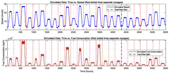
Figure 1.
Raw simulated data.
4.1.3. Data Pre-Processing
The raw generated fuel consumption data were directly utilized as input for the majority of the predictive models employed in this study. For the support vector regression (SVR) component within the proposed DGM-SVR hybrid model, its input—specifically, the residual sequence generated by the dynamic grey model (DGM)—was subjected to internal standardization prior to training. This was implemented using the Standardize = true option within MATLAB’s fitrsvm function, adhering to standard practice for SVR algorithms to potentially enhance training efficiency and model performance. No additional explicit normalization was applied to the other baseline models (StaticGM, DGM, MA) in their implementation for this research.
Based on the simulation settings and output logs, the entire dataset, comprising 6000 data points, was chronologically partitioned into the training and testing sets:
- The training set consisted of data from the initial 18 voyages, totaling 4320 data points (time steps 1 to 4320). This set was used for model parameter estimation (specifically for SVR) and for the initial establishment and subsequent rolling updates of the dynamic models.
- The test set included data from the subsequent 7 voyages, totaling 1680 data points (time steps 4321 to 6000). This set was reserved for evaluating the models’ generalization capability on unseen data, with a particular focus on assessing their effectiveness in predicting fuel consumption surges during high-speed maneuvers. The partition is visually indicated in Figure 1 by the bold black dashed line.
4.2. Experimental Setup
4.2.1. Evaluation Indicators
To comprehensively evaluate and compare the performance of the different forecasting models, two widely adopted metrics were selected, assessing accuracy from the perspectives of both relative and absolute error:
The mean absolute percentage error (MAPE) is calculated as follows:
The MAPE quantifies the average percentage deviation of predictions from the actual values, facilitating comparison across different scales. However, it is sensitive to actual values that are zero or close to zero.
The root mean square error (RMSE) is calculated as follows:
The RMSE measures the square root of the average squared differences between the predicted and actual values. It reflects the overall magnitude of prediction errors and is particularly sensitive to large deviations [20]. The units of RMSE are consistent with the original data (kg/h).
These metrics were computed for both the fitting performance on the training set and the predictive performance on the test set.
4.2.2. Compared Models
To demonstrate the efficacy of the proposed hybrid approach, its performance was benchmarked against three baseline models:
- Static GM (1,1) (StaticGM). A single, standard GM (1,1) model built using the entire training dataset. This represents the fundamental grey prediction methodology.
- Rolling GM (1,1) (DGM). A GM (1,1) model implemented with a rolling window mechanism. This dynamic approach aims to improve adaptability to time-varying system characteristics.
- Moving average (MA). A common baseline time series forecasting technique where the prediction for the next time step is the arithmetic mean of a fixed number of an N receding observations. The window size N for MA was set to 10.
The proposed approach, referred to as the DGM-SVR hybrid model (DGM-SVR), integrates the baseline forecasts generated by the rolling GM (1,1) with supplementary predictions of its residuals using a support vector regression (SVR) model.TABLKE.
Specifically, the DGM (1,1) was implemented with a rolling window of N = 10 data points, a choice validated using preliminary experiments to ensure a balance between adaptability and model robustness. The SVR module utilized a radial basis function (RBF) kernel, with input features comprising the previous M = 5 lagged residuals from the DGM predictions. Hyperparameters for SVR—including the regularization parameter (C), the kernel width, and the epsilon for the epsilon-insensitive loss function—were systematically tuned via grid search and k-fold cross-validation on the training set, with the objective of minimizing the root mean square error (RMSE).
5. Results and Analysis
Based on the experimental setup described above, all models were executed, yielding corresponding prediction results and performance metrics. The subsequent analysis examines the models’ performance from two key perspectives: overall predictive accuracy and the specific capability to forecast the identified fuel consumption surge events.
5.1. Comparative Analysis of the Overall Prediction Accuracy
Table 1 summarizes the MAPE and RMSE metrics of the four models on the training and test sets. Figure 2 visualizes the MAPE and RMSE comparisons on the test set in the form of bar charts, respectively.

Table 1.
Model comparison.
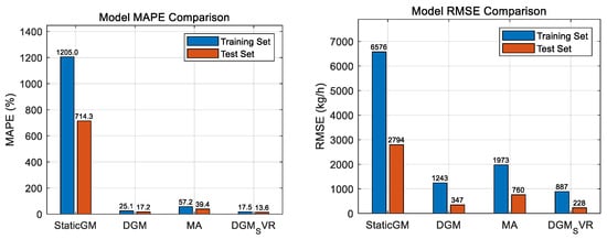
Figure 2.
Model MAPE comparison and model RMSE comparison.
- (1)
- The StaticGM model performed the worst: its MAPE and RMSE values were the highest among all the models, both on the training set and on the test set. Especially in the training set, the MAPE was over 1200% and the RMSE was over 6500, and in the test set, the MAPE was over 700% and the RMSE was close to 2800, which indicates that the static GM (1,1) model was completely unable to adapt to the dynamics and sudden changes of the fuel consumption data, and its prediction result is basically invalid.
- (2)
- DGM and MA models were improved but still insufficient: compared with StaticGM, the performance of the DGM (rolling GM (1,1)) and MA (sliding average) models significantly improved. The DGM outperformed the MA on the test set (MAPE 17.23% vs. 39.35%, RMSE 346.58 vs. 759.70), which indicates that the rolling grey model has an advantage over simple sliding averages in capturing dynamic trends. However, their error levels were still high, especially in the face of transient fuel consumption spikes.
- (3)
- Optimal performance of the DGM-SVR model: the hybrid DGM-SVR model proposed in this paper achieved the best performance on all metrics. The MAPE of DGM-SVR decreased to 13.62% and the RMSE decreased to 228.02 kg/h. Compared to the next-best-performing DGM model, the MAPE of DGM-SVR decreased by about 21% and the RMSE decreased by about 34% on the test set. This indicates that the DGM-SVR hybrid strategy significantly improves the overall prediction accuracy. Its fitting accuracy on the training set is also better than that of other models, and the training error and test error are closer, indicating that the model has better generalization ability.
5.2. Performance Comparison of Prediction Models for Transient Fuel Consumption Spikes
While overall accuracy metrics are important, this study was more concerned with the model’s ability to predict transient fuel consumption spikes caused by high-speed maneuvers. To this end, we focused on analyzing the model’s prediction curves and error performance on the test set.
Figure 3 shows the predicted values of each model during the test set (time points 4321 to 6000) compared to the actual fuel consumption (black solid line).
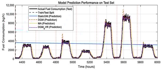
Figure 3.
Model prediction performance on the test set.
- StaticGM (blue solid line). The prediction result is almost a horizontal line, completely ignoring the dynamics of fuel consumption and all spikes.
- MA (yellow dotted line). The predicted curve is relatively smooth and follows the trend of fuel consumption, but lags behind the actual change and seriously underestimates the height of fuel consumption spikes and “flattens” them.
- DGM (red dashed line). Compared to MA, the prediction curve of the DGM better follows the baseline change in fuel consumption and responds to spikes. However, at the spikes, the predicted value of the DGM was still significantly lower than the actual peak, and there may be some delay or oscillation in the rising and falling phases of the spikes.
- DGM_SVR (purple dashes). The predicted curve of this model has the best agreement with the actual fuel consumption curve. Especially in the fuel consumption spike region, DGM-SVR is able to capture the magnitude and shape of the spike more accurately, and its predicted peak heights are much closer to the actual values than those of the DGM and the MA, and it responds more quickly to the rapid rise and fall process of the spike. This visually demonstrates the superiority of DGM-SVR in predicting sudden changes in fuel consumption.
Figure 4 plots the prediction error (actual—predicted) over time for each model on the test set.
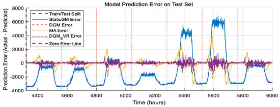
Figure 4.
Model prediction error on the test set.
- The error for StaticGM is large and fluctuates with the actual value.
- The errors for the MA and the DGM are relatively small during the smooth phase, but increase significantly during fuel consumption spikes, creating a distinct positive error peak (indicating that the predicted value is lower than the actual value). The error peaks for the DGM are typically smaller than for the MA.
- The prediction error of DGM_SVR remains relatively low throughout the test set, and the error fluctuation is significantly smaller than that of the DGM and the MA even during fuel consumption spikes. This suggests that the prediction results of DGM-SVR are more stable and accurate, especially in the critical spike region.
Figure 5 shows the histograms of the probability density distribution of the prediction errors of the three models, DGM, MA, and DGM-SVR, on the test set. Ideally, the errors should be centrally distributed around zero, with a mean close to zero.
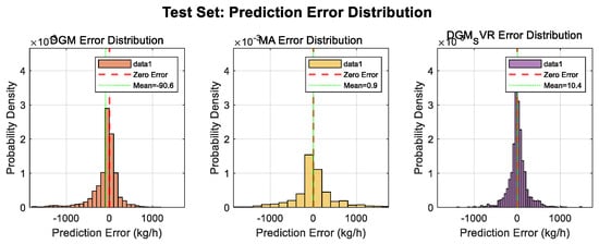
Figure 5.
Prediction error distribution on the test set.
The error distribution of the MA was relatively wide.
Although the error distribution of the DGM was also concentrated near zero, its mean (about −90.6, as shown in the legend) was significantly away from zero, corroborating its tendency to systematic underestimation (especially of spiking).
The error distribution of DGM_SVR was most centrally distributed near zero, with a higher and narrower pattern, and its mean (legend shows ca. 10.4) was also closest to zero. This further confirms the smaller error and lower bias of the DGM-SVR predictions.
Figure 6 illustrates the correspondence between the predicted and actual values for each model on the test set. Ideally, the scatter points should be closely distributed around the diagonal (y = x).
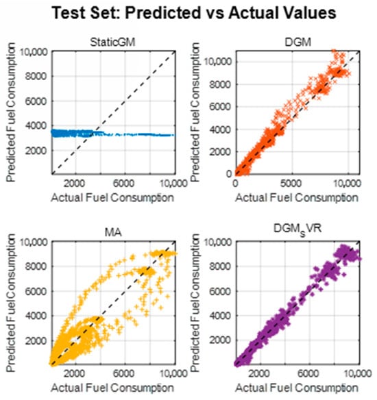
Figure 6.
Predicted vs. actual values on the test set.
The points for StaticGM are far from the diagonal.
The points of the MA and the DGM, although roughly trending diagonally, are more widely scattered, especially in the high fuel consumption region (corresponding to spikes) away from the diagonal.
The points of DGM_SVR are most closely clustered around the diagonal, covering the entire range from low to high fuel consumption (spikes). This indicates that the predicted values of DGM-SVR have the best agreement with the actual values.
6. Discussion
The empirical analysis conducted in this study provides compelling evidence for the efficacy of the proposed DGM-SVR hybrid model in addressing the intricate challenge of predicting ship fuel consumption, particularly under dynamic conditions involving high-speed maneuvers. The results unequivocally demonstrate that the DGM-SVR framework achieves superior performance compared to standalone static GM (1,1), moving average (MA), and even dynamic DGM (1,1) models, both in terms of overall predictive accuracy and, critically, in the ability to capture the transient fuel consumption spikes associated with maneuvering operations.
The pronounced underperformance of the static GM (1,1) model underscores its inherent inadequacy for modeling time series characterized by significant non-stationarity and abrupt changes, confirming the necessity for dynamic or adaptive approaches. While the MA and DGM models offered substantial improvements over the static baseline, their limitations became apparent when confronted with the sharp fuel consumption surges. The MA model, by its nature, tends to smooth out fluctuations, leading to significant underestimation and phase lag during spike events. The DGM (1,1), despite its rolling mechanism designed to adapt to baseline drift, still exhibited a tendency to underestimate peak magnitudes and react with a noticeable delay to the onset and cessation of these fuel spikes. This observation aligns with the theoretical understanding that grey models, while effective for trend extrapolation from limited data, possess inherent smoothing characteristics derived from their exponential fitting process, making them less adept at replicating sharp, transient phenomena [8]. The negative mean error observed for the DGM model in Figure 5 further corroborates this systematic underestimation, particularly of the spike peaks.
In stark contrast, the DGM-SVR hybrid model demonstrated a markedly improved predictive fidelity, particularly during the critical spike intervals. As visualized in Figure 3, the DGM-SVR predictions closely tracked the actual fuel consumption profile, capturing the magnitude and rapid dynamics of the surges with significantly higher accuracy than the other models. This is further substantiated by the substantially lower prediction errors during spike periods, the more tightly clustered and zero-centered error distribution, and the superior alignment of predicted versus actual values across the entire consumption range, including the high-consumption spike regions. The significant reductions in test set MAPE (21%) and RMSE (34%) relative to the next-best DGM model highlight the substantial contribution of the SVR component.
This enhanced performance can be attributed to the synergistic architecture of the hybrid model, effectively leveraging the complementary strengths of its constituent parts. The DGM component successfully captures the underlying dynamic trend and baseline drift of the fuel consumption using its rolling window mechanism, providing a competent initial forecast. The SVR component then focuses on modeling the residual sequence generated by the DGM. This residual series inherently contains the complex, non-linear information that the DGM failed to capture—predominantly the high-frequency, transient spike characteristics. SVR, with its robust capability to model complex non-linear relationships based on statistical learning theory and the structural risk minimization principle [21], proves highly effective in learning and predicting these residual patterns, thereby correcting the DGM’s shortcomings, especially in the spike regions. The hybrid strategy thus decomposes the complex prediction task into two more manageable sub-problems: trend forecasting (DGM) and residual/spike modeling (SVR), leading to a more accurate overall prediction.
The practical implications of these findings are significant for maritime operations management. Accurate prediction of fuel consumption, including transient surges during maneuvers, is paramount for optimizing voyage planning, enhancing energy efficiency initiatives (EEOI, CII compliance), ensuring logistical preparedness, and maintaining operational integrity, particularly for naval vessels where endurance and tactical capability are critical. The ability of the DGM-SVR model to provide more precise forecasts, especially during demanding operational phases, offers valuable support for decision-making regarding mission feasibility, optimal speed profiles, and scheduling of bunkering operations, potentially mitigating risks associated with unexpected fuel depletion.
However, it is important to acknowledge the limitations of this study. The current analysis relies on simulated data. While this data was designed to replicate key characteristics such as baseline drift and transient fuel spikes, it inevitably simplifies the multifaceted complexities of real-world maritime operations. Factors such as varying sea states, dynamic changes in vessel loading and trim, progressive hull fouling, specific engine performance curves and degradation, auxiliary system consumption, and unpredictable human operational factors were not explicitly modeled. Consequently, the model’s performance on real-world data, which is inherently subject to environmental noise, sensor inaccuracies, hardware variability, and operational anomalies, remains to be thoroughly investigated. The generalizability of the current findings would be significantly strengthened by validation against such operational datasets.
Future research should prioritize validating and refining the DGM-SVR model using extensive real-world operational data collected from diverse vessel types under a wide spectrum of operating conditions. This would also allow for an assessment of the model’s robustness against environmental noise and operational variability. Incorporating additional relevant input variables (e.g., speed over ground, acceleration, draft, trim, sea state parameters, engine RPM) into a multivariate prediction framework could further enhance predictive accuracy. Furthermore, while SVR proved effective for modeling residuals in this study, exploring alternative or complementary methods for capturing fuel spike dynamics is warranted. For instance, deep learning models like Long Short-Term Memory (LSTM) networks or Gated Recurrent Units (GRUs), known for their proficiency in handling temporal dependencies in sequential data [22], could be investigated for modeling the residual series or even as part of an end-to-end hybrid architecture. A comparative analysis against such advanced neural network-based approaches would provide valuable insights into the optimal strategies for this specific prediction task. Adaptive methods for dynamically optimizing the DGM window size and SVR (or alternative model) hyperparameters based on evolving data characteristics also represent a promising research direction.
In summary, this study successfully demonstrates that the proposed DGM-SVR hybrid modeling approach represents a significant advancement in predicting ship fuel consumption time series characterized by both baseline drift and transient spikes. By effectively combining the trend-following capabilities of DGM with the non-linear residual modeling power of SVR, the model offers enhanced accuracy and responsiveness, particularly for the challenging prediction of fuel surges during high-speed maneuvers, holding considerable promise for applications in ship energy management and operational decision support.
7. Conclusions
This study introduced and empirically validated a novel hybrid prediction model, DGM-SVR, designed to address the complex challenge of accurately forecasting ship fuel consumption, particularly the coexisting baseline drift and transient spikes prevalent during high-speed maneuvering scenarios. Traditional models often falter in such dynamic conditions, as highlighted in the Introduction. The proposed DGM-SVR method synergistically integrates a rolling Dynamic Grey Model (DGM (1,1)) for adaptive tracking of the fuel consumption baseline trend with Support Vector Regression (SVR) for effectively learning and predicting the DGM-generated residual sequence, which predominantly encapsulates the high-amplitude, maneuver-induced fuel spikes.
The empirical analysis, conducted on a simulated dataset meticulously designed to reflect these challenging operational characteristics, demonstrated the DGM-SVR model’s significant superiority. Compared to standalone DGM (1,1), moving average (MA), and static GM (1,1) models, the DGM-SVR hybrid consistently achieved the highest overall prediction accuracy, evidenced by the lowest mean absolute percentage error (MAPE) and root mean square error (RMSE) on the test set. More critically, the DGM-SVR model exhibited a pronounced capability in forecasting the timing, magnitude, and morphology of abrupt fuel consumption spikes, thereby effectively overcoming a key limitation of the benchmarked single-paradigm models.
The principal contribution of this research is the development and successful application of a DGM-SVR hybrid architecture specifically tailored to the nuanced dynamics of ship fuel consumption, particularly its transient spike behavior. The findings indicate that this “trend + residual” decomposition strategy provides a more robust, reliable, and precise method for dynamic ship fuel consumption forecasting. This enhanced predictive capability has considerable practical implications for optimizing ship voyage planning, improving fuel management strategies, enhancing logistical support for naval operations, and ultimately contributing to the operational effectiveness, energy efficiency, and economic viability of maritime activities.
Future research endeavors should prioritize the validation and refinement of the DGM-SVR model using extensive real-world operational data from diverse vessel types and under a wider spectrum of operating conditions. Further investigations could also explore the incorporation of multivariate inputs and advanced residual modeling techniques to potentially enhance its predictive power and robustness in complex maritime environments.
Author Contributions
Conceptualization, J.C. and Y.P.; methodology, J.C.; software, J.C.; validation, J.C. and Y.P.; formal analysis, J.C.; investigation, Y.P.; resources, Y.P.; data curation, J.C.; writing—original draft preparation, J.C.; writing—review and editing, Y.P.; supervision, Y.P. All authors have read and agreed to the published version of the manuscript.
Funding
This research received no external funding.
Institutional Review Board Statement
Not applicable.
Informed Consent Statement
Not applicable.
Data Availability Statement
The original contributions presented in this study are included in the article. Further inquiries can be directed to the corresponding author.
Conflicts of Interest
The authors declare no conflict of interest.
References
- Horne, F.J. Naval Logistics Administration. Public Admin. Rev. 1945, 5, 312–316. [Google Scholar] [CrossRef]
- Uyanık, T.; Karatuğ, Ç.; Arslanoğlu, Y. Machine learning approach to ship fuel consumption: A case of container vessel. Transp. Res. Part D 2020, 84, 102389. [Google Scholar] [CrossRef]
- Chen, Y.; Sun, B.; Xie, X.; Li, X.; Li, Y.; Zhao, Y. Short-term forecasting for ship fuel consumption based on deep learning. Ocean Eng. 2024, 301. [Google Scholar] [CrossRef]
- Yao, Z.; Ng, S.H.; Lee, L.H. A study on bunker fuel management for the shipping liner services. Comput. Oper. Res. 2012, 39, 1160–1172. [Google Scholar] [CrossRef]
- Hu, Z.; Zhou, T.; Zhen, R.; Jin, Y.; Li, X.; Osman, M.T. A two-step strategy for fuel consumption prediction and optimization of ocean-going ships. Ocean Eng. 2022, 249, 110904. [Google Scholar] [CrossRef]
- Baldi, F.; Ahlgren, F.; Melino, F.; Gabrielii, C.; Andersson, K. Optimal load allocation of complex ship power plants. Energy Convers. Manag. 2016, 124, 344–356. [Google Scholar] [CrossRef]
- Rudzki, K.; Gomulka, P.; Hoang, A.T. Optimization model to manage ship fuel consumption and navigation time. Pol. Marit. Res. 2022, 29, 141–153. [Google Scholar] [CrossRef]
- Christodoulos, C.; Michalakelis, C.; Varoutas, D. Forecasting with limited data: Combining ARIMA and diffusion models. Technol. Forecast. Soc. Change 2010, 77, 558–565. [Google Scholar] [CrossRef]
- Jeutsa, A.K.; Kibong, M.T.; Diboma, B.S.; Sapnken, F.E.; Noumo, P.G.; Tamba, J.G. On the Limitations of Univariate Grey Prediction Models: Findings and Failures. Comput. Math. Methods 2024, 1, 9961208. [Google Scholar] [CrossRef]
- Han, Z.; Zhao, J.; Leung, H.; Ma, K.F.; Wang, W. A review of deep learning models for time series prediction. IEEE Sens. J. 2019, 21, 7833–7848. [Google Scholar] [CrossRef]
- Wang, H.; Zhou, H.; Cheng, S. Dynamical system prediction from sparse observations using deep neural networks with Voronoi tessellation and physics constraint. Comput. Methods Appl. Mech. Eng. 2024, 432, 117339. [Google Scholar] [CrossRef]
- Zhou, H.; Cheng, S.; Arcucci, R. Multi-fidelity physics constrained neural networks for dynamical systems. Comput. Methods Appl. Mech. Eng. 2024, 420, 116758. [Google Scholar] [CrossRef]
- Müller, K.R.; Smola, A.J.; Rätsch, G.; Schölkopf, B.; Kohlmorgen, J.; Vapnik, V. Predicting time series with support vector machines. In International Conference on Artificial Neural Networks; Springer: Berlin/Heidelberg, Germany, 1998; pp. 999–1004. [Google Scholar]
- Shi, J.; Leau, Y.B.; Li, K.; Obit, J.H. A comprehensive review on hybrid network traffic prediction model. Int. J. Electr. Comput. Eng. 2021, 11, 1450. [Google Scholar] [CrossRef]
- Aminikhanghahi, S.; Cook, D.J. A survey of methods for time series change point detection. Knowl. Inf. Syst. 2017, 51, 339–367. [Google Scholar] [CrossRef] [PubMed]
- Capezza, C.; Coleman, S.; Lepore, A.; Palumbo, B.; Vitiello, L. Ship fuel consumption monitoring and fault detection via partial least squares and control charts of navigation data. Transp. Res. Part D 2019, 67, 375–387. [Google Scholar] [CrossRef]
- Li, C.; Qi, Q. A novel hybrid grey system forecasting model based on seasonal fluctuation characteristics for electricity consumption in primary industry. Energy 2024, 287, 129585. [Google Scholar] [CrossRef]
- Bishop, C.M.; Nasrabadi, N.M. Pattern Recognition and Machine Learning; Springer: New York, NY, USA, 2006; Volume 4. [Google Scholar]
- Vapnik, V.N. An overview of statistical learning theory. IEEE Trans. Neural Netw. 1999, 10, 988–999. [Google Scholar] [CrossRef] [PubMed]
- Hastie, T.; Tibshirani, R.; Friedman, J.H. The Elements of Statistical Learning: Data Mining, Inference, and Prediction; Springer: New York, NY, USA, 2009; Volume 2. [Google Scholar]
- Tran, N.K.; Kühle, L.C.; Klau, G.W. A critical review of multi-output support vector regression. Pattern Recognit. Lett. 2024, 178, 69–75. [Google Scholar]
- Greff, K.; Srivastava, R.K.; Koutník, J.; Steunebrink, B.R.; Schmidhuber, J. LSTM: A search space odyssey. IEEE Trans. Neural Netw. Learn. Syst. 2016, 28, 2222–2232. [Google Scholar] [CrossRef] [PubMed]
Disclaimer/Publisher’s Note: The statements, opinions and data contained in all publications are solely those of the individual author(s) and contributor(s) and not of MDPI and/or the editor(s). MDPI and/or the editor(s) disclaim responsibility for any injury to people or property resulting from any ideas, methods, instructions or products referred to in the content. |
© 2025 by the authors. Licensee MDPI, Basel, Switzerland. This article is an open access article distributed under the terms and conditions of the Creative Commons Attribution (CC BY) license (https://creativecommons.org/licenses/by/4.0/).