Abstract
This paper presents a non-fragile observer-based dissipative control strategy for the suspension systems of electric vehicles equipped with in-wheel motors, accounting for input delays, actuator faults, and observer gain uncertainty. Traditional control approaches—such as , passive control, and robust feedback schemes, often address these challenges in isolation and with increased conservatism. In contrast, this work introduces a unified framework that integrates fault-tolerant control, delay compensation, and robust state estimation within a dissipativity-based setting. A novel dissipativity analysis tailored to Electric Vehicle Active Suspension Systems (EV-ASSs) is developed, with nonzero delay bounds explicitly incorporated into the stability conditions. The observer is designed to ensure accurate state estimation under gain perturbations, enabling robust full-state feedback control. Stability and performance criteria are formulated via Linear Matrix Inequalities (LMIs) using advanced integral inequalities to reduce conservatism. Numerical simulations validate the proposed method, demonstrating effective fault-tolerant performance, disturbance rejection, and precise state reconstruction, thereby extending beyond the capabilities of traditional control frameworks.
1. Introduction
The global move towards green transportation has fueled extensive development of electric vehicles (EVs), and innovative measures focusing on environmental conservation, energy saving, and driving experience have accelerated. Among such developments, the evolution of In-Wheel Motor (IWM)-powered electric vehicles has attracted great attention as a means of optimizing space, allowing independent control of all four wheels, and providing the ability to regenerate energy [1,2]. Unlike conventional drivetrain architectures, IWMs integrate the propulsion unit directly within the wheel assembly, eliminating the need for mechanical components such as gearboxes and drive shafts. However, this structural transformation comes at the cost of a substantial increase in the unsprung mass, which adversely impacts ride comfort, road holding, and handling stability.
In addition to increased unsprung mass, IWMs introduce unique dynamic challenges such as torque ripple, unbalanced electromagnetic forces, and nonlinear motor dynamics. These factors collectively exacerbate the vibrational behavior of the vehicle, potentially degrading passenger comfort and compromising safety. Therefore, developing advanced control strategies that effectively address these dynamics is critical for realizing the full potential of IWM-based EVs, which can be witnessed in [3,4].
Active suspension systems (ASSs) have emerged as a promising solution to mitigate these adverse effects. By actively modulating suspension forces through actuators, ASSs enable superior ride quality, enhanced road holding, and improved handling performance compared to passive or semi-active suspension systems. Various actuator technologies, including hydraulic, pneumatic, and electromagnetic actuators, have been explored to realize active suspensions; each of these technologies has its advantages and limitations.
We examined numerous published works on the control strategies for ASSs. For example, a hybrid control scheme employing fault-tolerant control and state feedback control has been proposed in [5], where the ASS is subjected to actuator fault and various external disturbances. On the other hand, ref. [6] discusses non-fragile fault-tolerant control for vehicle suspensions with quantization of input signals. The authors of [7] designed a dynamic feedback controller, in which a half-vehicle ASS is subjected to input delay. Time-delay effects in suspension dynamics have been effectively addressed in prior works through compensation strategies and stability analysis, as discussed in [8]. Robust control designs incorporating fuzzy logic and optimal feedback strategies for active suspension systems have been explored in depth in [9]. Recent studies have proposed adaptive event-triggered output feedback methods using interval type 2 fuzzy models to handle nonlinearities in suspension systems [10]. The integration of dynamic event-triggered mechanisms with finite-time neural control has been demonstrated to address performance constraints in active suspension systems [11]. Fault-tolerant control schemes using reliable fuzzy frameworks have been developed to mitigate actuator failures in active suspension setups [12]. Recent advancements in suspension control have increasingly focused on intelligent and hybrid strategies to improve vibration isolation and fault resilience under realistic operating conditions. Ref. [13] proposed a multi-agent reinforcement learning framework for regenerative active suspension, demonstrating improved vibration control by leveraging distributed learning agents. Shen et al. [14] introduced a fractional-order biquadratic electrical network in a mechatronic ISD suspension system, showing effective vibration suppression through advanced fractional-calculus-based modeling. In the context of high-speed maglev systems, the study [15] applied a combined skyhook–groundhook damping optimization technique for superconducting suspensions, highlighting the adaptability of hybrid control strategies in dynamic environments. Additionally, ref. [16] explored the design and optimization of semi-active suspensions for railway applications, providing foundational insight into performance trade-offs in large-scale transport systems. These studies collectively underscore the growing emphasis on intelligent, robust, and application-specific suspension designs, which align with the objectives pursued in this work.
Despite extensive research on active suspension control strategies, several critical issues remain underexplored, particularly in the context of IWM-driven EVs. First, input time delays, arising from sensor measurements, communication networks, computation, or actuator dynamics, can significantly deteriorate system performance and may even destabilize the control system if not properly addressed [17,18]. Second, actuator faults, which can consist of partial loss of effectiveness or complete failure, are inevitable in practical systems and can severely compromise the system’s fault tolerance and robustness [19]. As a result, ensuring stability and acceptable performance under such adverse conditions is vital for the safe and reliable operation of modern EVs.
Furthermore, direct measurement of all system states is often impractical or cost-prohibitive due to sensor limitations, noise, or economic constraints. To overcome this, observer-based control designs have been widely adopted, wherein the system states are estimated using limited output measurements [20,21]. Observer-based control plays a crucial role in modern control systems where it is often impractical or costly to measure all the system states directly. By reconstructing the unmeasured states from available outputs, an observer enables the implementation of full-state feedback control strategies without requiring direct access to every state variable. This approach enhances system performance, allows fault-tolerant control, and supports real-time implementation in resource-constrained environments. Moreover, it provides a framework for dealing with uncertainties and disturbances, ensuring robustness and reliability of the closed-loop system. In this regard, non-fragile observer designs have garnered interest, as they offer resilience against perturbations and uncertainties in observer gains—a desirable property in real-world applications where exact modeling is often infeasible [22].
Another critical consideration in control system design is the system’s ability to dissipate energy and withstand external disturbances. Traditional stability analysis ensures that the system trajectories converge to equilibrium; however, it does not explicitly guarantee performance against disturbances. This motivates the adoption of dissipative control frameworks, where the system is designed to dissipate or neutralize external energy inputs effectively. Dissipativity encompasses and generalizes several conventional control objectives, including performance, passivity, and robust stability, making it an indispensable tool for designing controllers that ensure both stability and robustness against external influences. On the other hand, stability analysis using Lyapunov–Krasovskii functionals (LKFs) is a powerful method for dealing with systems that involve time delays, such as delayed-feedback control or sampled-data systems [23]. Unlike classical Lyapunov methods, this approach constructs a functional that accounts for both the current and past states of the system, capturing the influence of delays explicitly. By ensuring that the derivative of the functional along the system trajectories is negative definite, one can establish sufficient conditions for the asymptotic stability or admissibility of the delayed system. This technique is widely used in control theory due to its ability to handle a broad class of delay-dependent and delay-independent stability problems with rigor and generality.
In the specific context of IWM-driven electric vehicles, ensuring dissipativity is important not only for disturbance rejection but also for energy-efficient operation, prolonged mechanical integrity, and passenger comfort and safety under a wide range of driving conditions and fault scenarios. Therefore, a robust dissipative control strategy that accounts for time delays, actuator faults, and modeling uncertainties becomes crucial.
Motivated by these challenges, this paper proposes a novel non-fragile observer-based dissipative control strategy for active suspension systems of electric vehicles equipped with in-wheel motors. This article presents several novel contributions to the analysis and control of delayed suspension systems, particularly within the framework of electric vehicle active suspension systems (EV-ASSs), under realistic operating constraints. The key contributions are summarized as follows:
- An observer-based dissipative control framework is developed to achieve robust state estimation and regulation.
- Nonzero delay bounds are explicitly considered, reflecting realistic actuator and communication delays.
- A novel dissipativity analysis is introduced for EV-ASSs, offering a new perspective not previously explored.
- Actuator faults and nonzero bounded input delays are jointly addressed through uncertainty modeling integrated into LMI conditions.
- Stability conditions are made less conservative by employing advanced integral inequality techniques.
- Simulation results validate the proposed approach, demonstrating accurate state estimation and fault analysis in different cases.
The remainder of the paper is organized as follows: Section 2 presents the system formulation, the modeling of the active suspension dynamics, and the performance requirements. Section 3 discusses the design of the non-fragile observer and the observer-based controller. Section 4 establishes the main theoretical results and stability proofs. Section 5 illustrates the simulation results and feasibility studies. Finally, Section 6 concludes the paper with potential directions for future research.
2. System Formulation
The dynamic equations of the ASS for the quarter-car model, along with the IWM dynamics, are given below and represented in Figure 1.
where
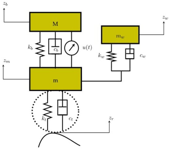
Figure 1.
Active suspension system for an EV with embedded in-wheel motors.
In the mathematical formulation of the suspension system, the subscripts b, w, and t are used to denote quantities related to the car body, the motor wheel, and the tire, respectively. The parameters and m represent the masses of the car body (sprung mass), the in-wheel motor assembly, and the tire (unsprung mass in contact with the road), respectively. The symbols k and c correspond to the stiffness and damping coefficients that characterize the elastic and dissipative properties of the suspension components. Specifically, and denote the stiffness and damping between the car body and the motor, and refer to those between the motor and the wheel, and and represent the stiffness and damping between the wheel and the road interface. Here, is the control input provided by the actuator.
Performance Requirements
For an active suspension to work effectively, the following requirements should be met:
- (i)
- Suspension deflection: The bound of the suspension stroke should not be greater than its maximum permissible value, i.e., .
- (ii)
- Road holding: To achieve sufficiently stable road holding, the dynamic load should be low when compared to the static load, i.e., , with gravity constant .
- (iii)
- Ride comfort: To achieve sufficient comfort during drives, the vertical body acceleration, , should be minimized.
Keeping these constraints in mind, the state vector, control output vector, and measurement output vector are taken, respectively, to be
= ,
= , and
= .
Thus, the following state-space equations are obtained:
where A = , = , = , , , , and .
3. Non-Fragile Observer
In order to estimate the states of system (2), a non-fragile observer is given as follows:
where is the state estimate vector, is the output estimate vector, L is the observer gain, and is the additive perturbation (in which , where M and N are real known constant matrices and J is the unknown matrix satisfying ).
Controller Design
In this work, a controller in faulty condition is to be investigated. The state feedback controller with the considered actuator fault parameter is designed as
where K is the controller gain to be designed and is the time-varying delay, whose derivative is bounded. The expression for this time-varying delay is explicitly stated in the simulation section. Moreover, the fault model is usually discussed in three cases:
- Case(1)
- When , the actuator force becomes completely zero, and thus, the active suspension turns into a passive one.
- Case(2)
- When , there occurs a partial fault in the actuator; in real applications, this case is the most common.
- Case(3)
- When , there exists no fault in the actuator, indicating ideal actuator performance, which is unnecessary to discuss here.
In this work, Case(2) is taken for study, and thus, replacing the actual control force will result in
The error is framed as , and the corresponding error system is given as
Definition 1.
By [24], if and are given matrices, then the closed-loop system (6) becomes dissipative if the following condition holds under a zero initial condition:
with the energy supply function and as dissipative index, where and are symmetric matrices and .
Remark 1.
By changing the values of the weight matrices and , the conventional control frameworks can be deduced as special cases:
- 1.
- If and , then dissipativity becomes performance;
- 2.
- If and , then dissipativity becomes passive performance;
- 3.
- If and , then dissipativity turns into mixed passive and performance, with .
Assumption 1.
The time-varying delay term has the boundary conditions and its derivative , where and φ are positive constants.
Remark 2.
In many existing studies, the lower bound of the time delay is typically assumed to be zero for mathematical simplicity. However, to more accurately replicate practical scenarios where delays are inherently non-negligible, this work considers a nonzero lower bound for the delay term, thereby offering a more realistic and robust modeling framework.
4. Main Results
Before moving to further discussions, let us define some vector notations for upcoming derivations. the block matrices , , , , , .
Lemma 1
([25]). For any matrix , along with the vector and a constant , if the matrix satisfies
then the following inequality holds true:
where
Lemma 2
([26]). For any scalars h and j with and for any symmetric matrix , along with a differentiable vector function , the following holds:
where
The following theorem will be applied to dissipativity and stability analysis of the closed-loop system.
Theorem 1.
The closed-loop quarter-vehicle ASS (6) with the proposed non-fragile observer (3) and the observer based controller (4) attains -dissipative stability if, for given positive scalars and , and given controller and observer gain matrices K and L, there ∃ symmetric positive matrices and , for , and any matrix of appropriate dimension, such that
, , the following LMI conditions hold:
where
Proof.
Construct the Lyapunov functional candidate as
where is the quadratic LKF and is the improved LKF, which are given as
By calculating the time derivative from (12) to (17) and employing Assumption 1, we obtain
Now, by Lemma 1, the integral term in (22) can be estimated as
where are defined in Lemma 1. Moreover, from Lemma 2, we can say that
The zero equation presented below holds for any matrices :
where .
By summing (18) to (26), we obtain
By adding to both sides, we get
where and the other vectors are as defined in Theorem 1.
By virtue of the Schur complement, if , then, from (28), we have
for any , which is guaranteed in the LMI (9). Under zero initial conditions, it is evident that
Thus, by Definition 1, dissipativity is satisfied. Unless , we get
This proves the asymptotic stability of the system. Next, the derivation of hard constraints (ii) and (iii) for the performance requirements follows. From (30), we have
where ,. Assuming , the following inequality can be obtained:
If , then, by the Schur complement, the constraints (ii) and (iii) are guaranteed in view of the LMI (10), which completes the proof. □
The following theorem helps to determine the controller and observer gain by means of appropriate transformation.
Theorem 2.
The closed-loop quarter vehicle ASS (6) with the proposed non-fragile observer (3) and the observer-based controller (4) attains - dissipative stability if, for given positive scalars , there ∃ symmetric positive matrices and , for , and any matrix with appropriate dimension, such that , , then the following LMI conditions hold:
where
Moreover, the gain matrices are given by and .
Proof.
Now take , and define , . Assuming , , follow the same procedure as in Theorem 1, and then left-multiply and right-multiply the LMI (9) by and its transpose on both sides to yield (34); similarly, left- and right-multiply the LMI (10) by and its transpose on both sides to yield (35). □
5. Simulation Results
In this section, numerical simulations are carried out to validate the effectiveness and robustness of the proposed non-fragile observer-based dissipative control strategy. The simulations are performed using MATLAB/Simulink with the system parameters, controller gains, observer gains, and scalar values described earlier. The system matrices are constructed based on the quarter-car model of the active suspension system integrated with the in-wheel motor dynamics, as detailed in Section 2. The physical parameters as taken from [27], such as mass, damping, and stiffness coefficients, are given in Table 1. The time-varying delay is given as , from which we get the respective upper and lower bounds. The designed state feedback controller gain K and observer gain L are obtained by solving the formulated Linear Matrix Inequalities (LMIs) ensuring -dissipativity. Furthermore, the scalar values associated with the LMI conditions are chosen as respectively, to ensure the feasibility and conservativeness of the stability conditions.
By solving Theorem 1, we obtain the corresponding controller and observer gain matrices:
The values of , M, N, and J are calculated as , and .

Table 1.
Description of the parameter values.
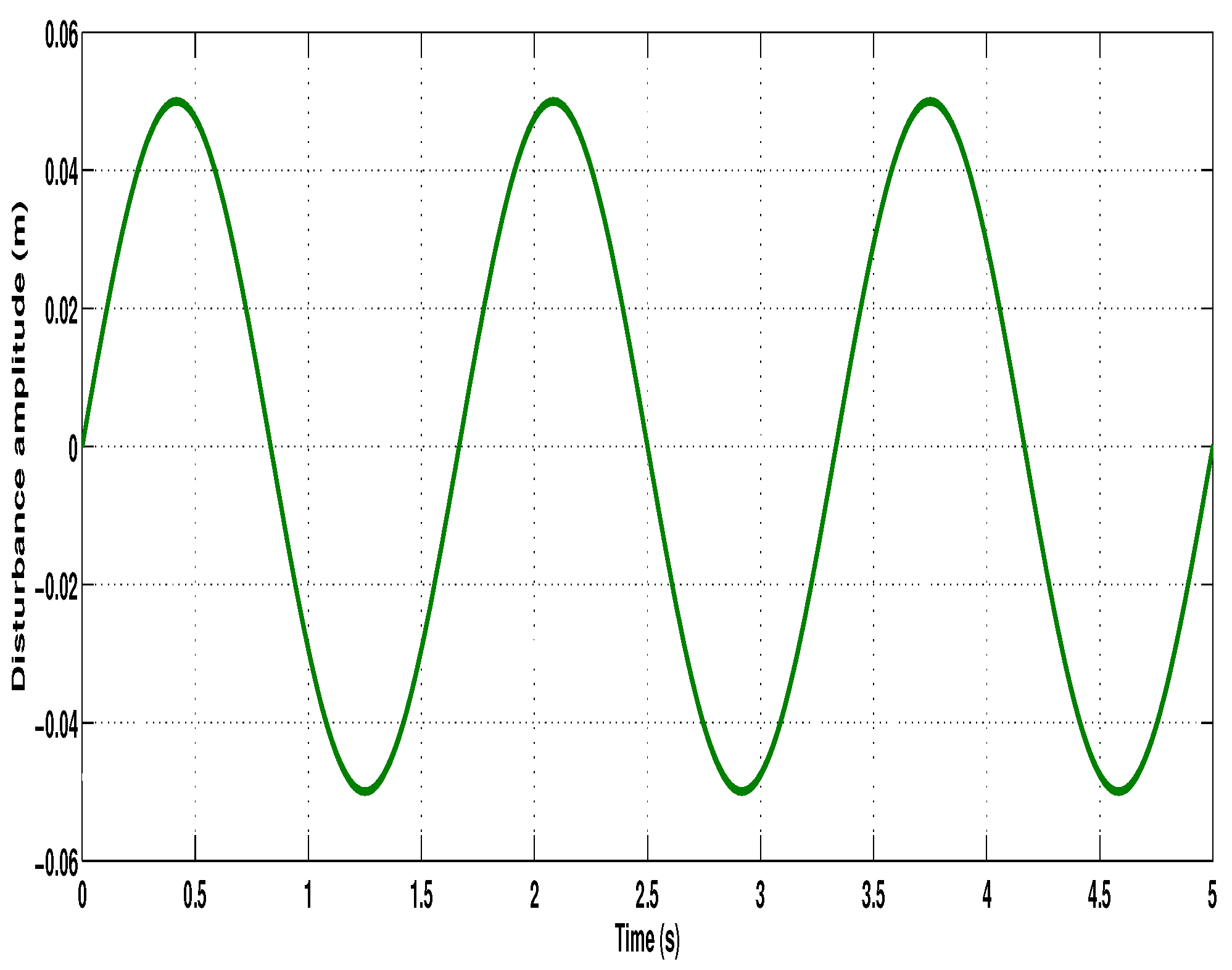
To evaluate the disturbance rejection capability of the suspension system, a bumpy road profile is considered. The road disturbance is modeled as a smooth bump of finite width and height, defined by a continuous piecewise function, given in Figure 2.
where r = 5 m, a = 0.1 m, and q = 30 km/h. The bump profile simulates a realistic road irregularity scenario commonly encountered during vehicle operation. The plot of the bump input shows a smooth rise and fall over a finite time horizon, which introduces transient dynamics into the suspension system. This input is critical in examining how effectively the suspension mitigates sudden external disturbances to maintain ride comfort and road holding.
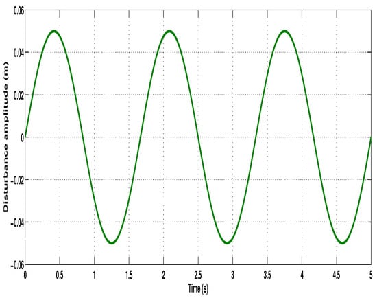
Figure 2.
Disturbance input.
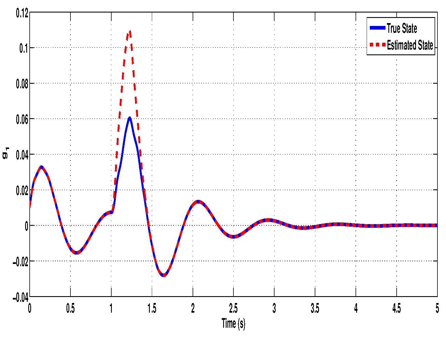
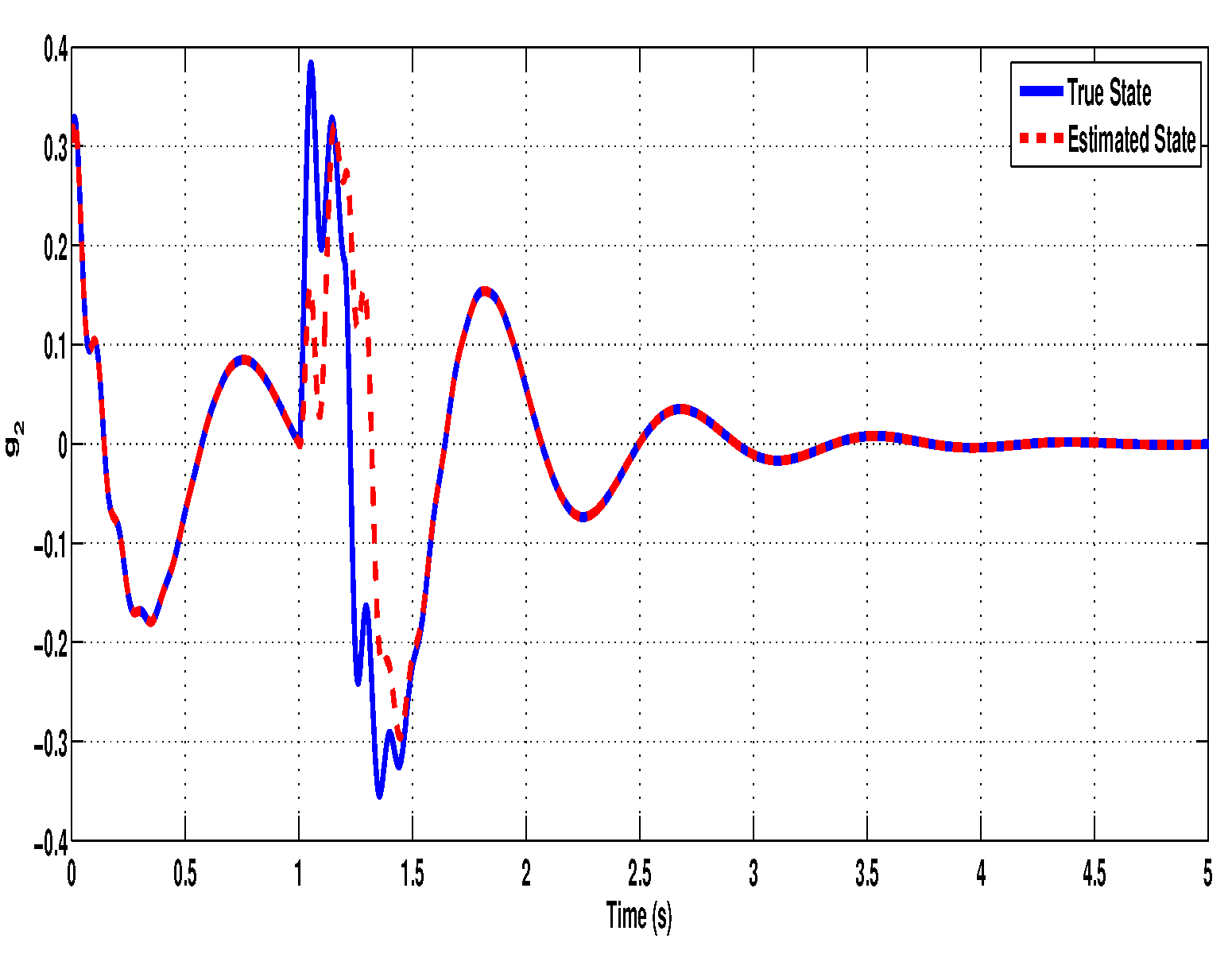
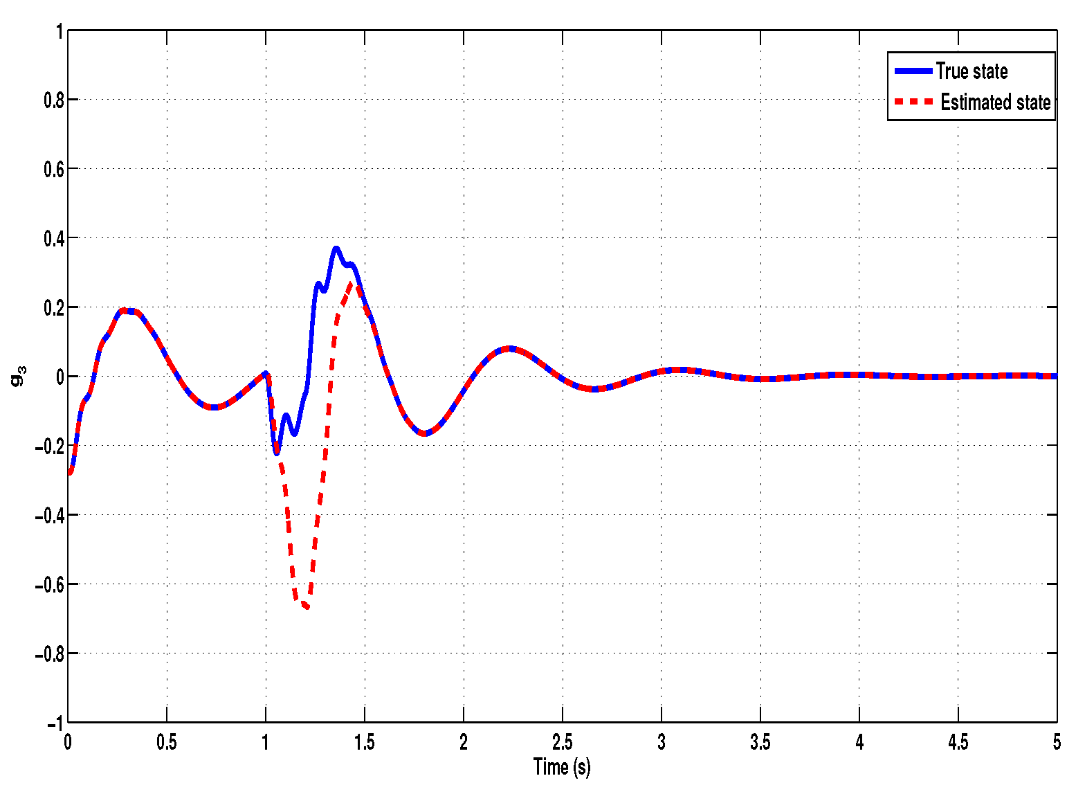
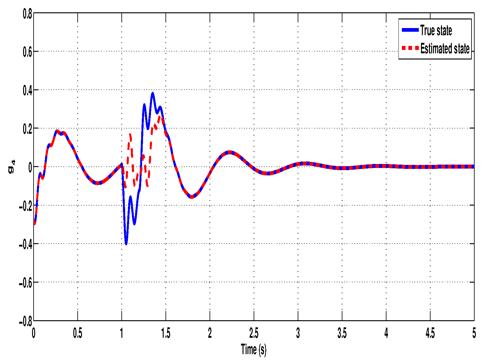
Further, the effectiveness of the proposed non-fragile observer is evaluated by comparing the true states of the system with the estimated states. Figure 3, Figure 4, Figure 5, Figure 6, Figure 7 and Figure 8 illustrate the time-domain performance of the proposed non-fragile observer in estimating the six key states of the quarter-car active suspension system integrated with an in-wheel motor. In Figure 3, the true and estimated trajectories of , representing the car body velocity, show near-perfect alignment, demonstrating the observer’s ability to reconstruct fast-changing dynamics with high fidelity. Figure 4 displays the comparison for , the relative displacement between the car body and the motor, where the observer accurately tracks suspension deflection, which is a critical metric for maintaining mechanical limits. Figure 5 corresponds to , the wheel velocity, and shows that the estimate closely follows the true dynamics, ensuring accurate feedback for road handling assessment. In Figure 6, the observer estimates the relative motion between the wheel and motor mass through state , again maintaining close agreement throughout the simulation. Figure 7 examines , the velocity of the motor mass, where the estimated response exhibits precise transient behavior and rapid convergence despite observer gain uncertainties. Finally, Figure 8 presents the estimation of , the displacement between the motor mass and the road profile, showing that the observer effectively captures external disturbance effects. Across all figures, the negligible estimation error and rapid convergence highlight the robustness and accuracy of the observer design, even under time-varying delays and additive perturbations in the gain matrix. To further assess the estimation performance, although the error state responses (defined as the difference between the true and estimated states) are not explicitly plotted, it is observed that the estimation errors converge rapidly toward zero. This behavior highlights the observer’s robustness and accuracy in reconstructing the full state vector necessary for feedback control.
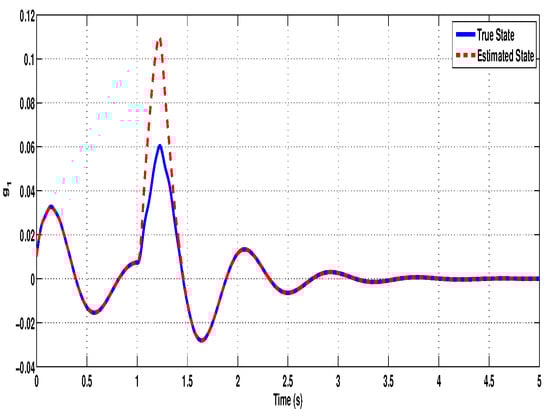
Figure 3.
Original and estimated responses of the state .
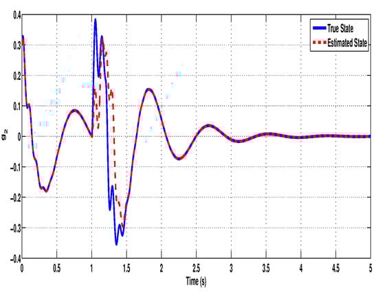
Figure 4.
Original and estimated responses of the state .

Figure 5.
Original and estimated responses of the state .
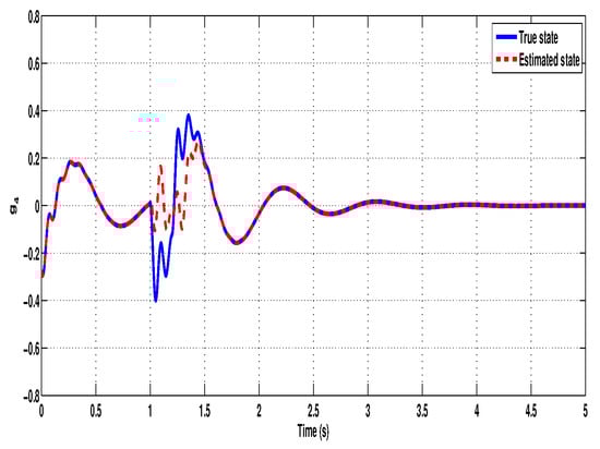
Figure 6.
Original and estimated responses of the state .
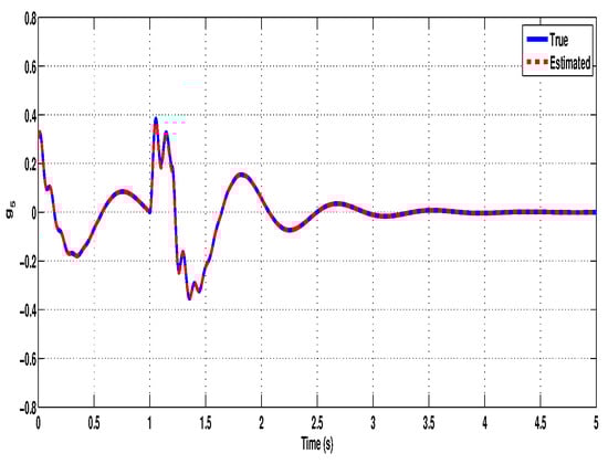
Figure 7.
Original and estimated responses of the state .
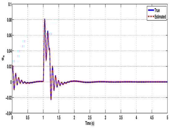
Figure 8.
Original and estimated responses of the state .
5.1. Effects of Uncertainty in Responses
To further assess the robustness of the proposed non-fragile observer-based control strategy, additional scenarios were simulated to evaluate the system’s performance in the presence and absence of uncertain conditions. In particular, the effects of observer gain perturbations and input delay were closely examined and simulated.
5.1.1. In the Presence of
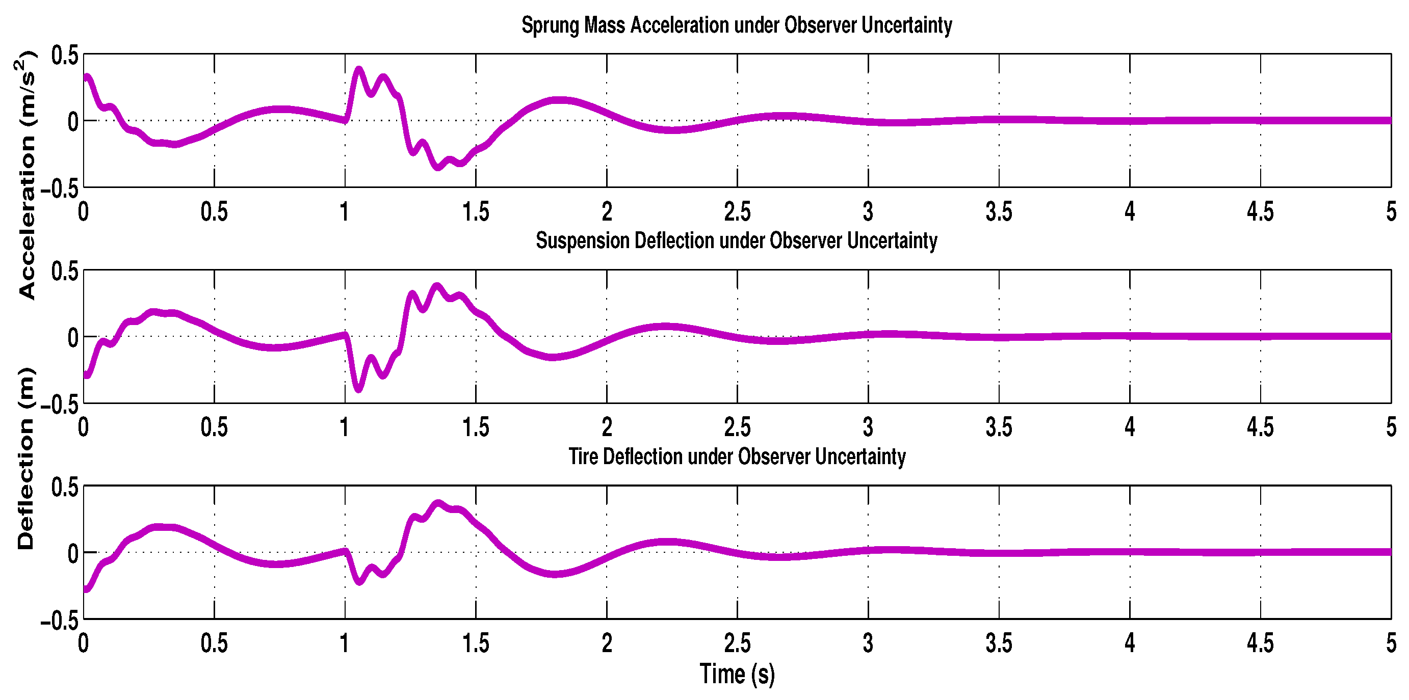
To analyze the robustness of the proposed design under uncertainty, a scenario involving intentional perturbations in the observer gain matrix was considered. Specifically, additive uncertainties were introduced into the nominal observer gain to evaluate the non-fragile nature of the proposed observer-based control strategy. Figure 9 illustrates the system’s output responses—such as sprung mass acceleration, suspension deflection, and tire deflection—under these uncertain observer gains. Compared to the nominal case shown in Figure 10, the system exhibits slight deviations in transient performance, including an increase in overshoot by approximately and a marginal increase in settling time by about 0.3 s. Despite these variations, the system maintains overall stability and acceptable dynamic behavior, with no signs of divergence or instability. These results validate the robustness of the proposed non-fragile design, confirming its effectiveness in tolerating observer gain perturbations and ensuring reliable performance under practical modeling uncertainties.
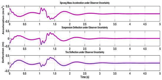
Figure 9.
Responses of the output in the presence of uncertain perturbation.
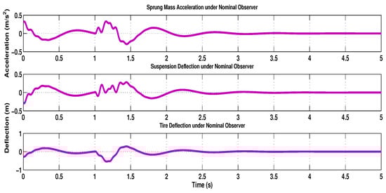
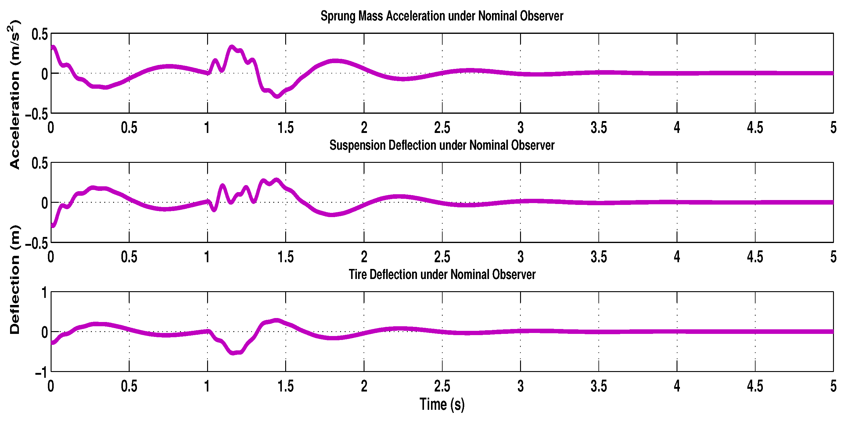
Figure 10.
Responses of the output in the absence of uncertain perturbation.
5.1.2. In the Absence of
For comparison, the system’s behavior under the nominal observer gain—i.e., in the absence of any uncertainty or perturbation—was also analyzed to establish a performance baseline. The output responses, presented in Figure 10, exhibit smooth dynamics with rapid convergence, minimal overshoot, and superior disturbance rejection across all measured states. These results highlight the optimal transient characteristics achievable with an accurately tuned observer, including tighter state estimation and improved control precision. Compared to the uncertain observer scenario (Figure 9), the nominal case demonstrates a more responsive system with reduced oscillations and faster settling, thereby underscoring the performance benefit of an ideal observer configuration. This comparison reinforces the value of robust observer design while also illustrating the upper performance bound under ideal conditions, validating both the non-fragile robustness and the optimality potential of the proposed approach.
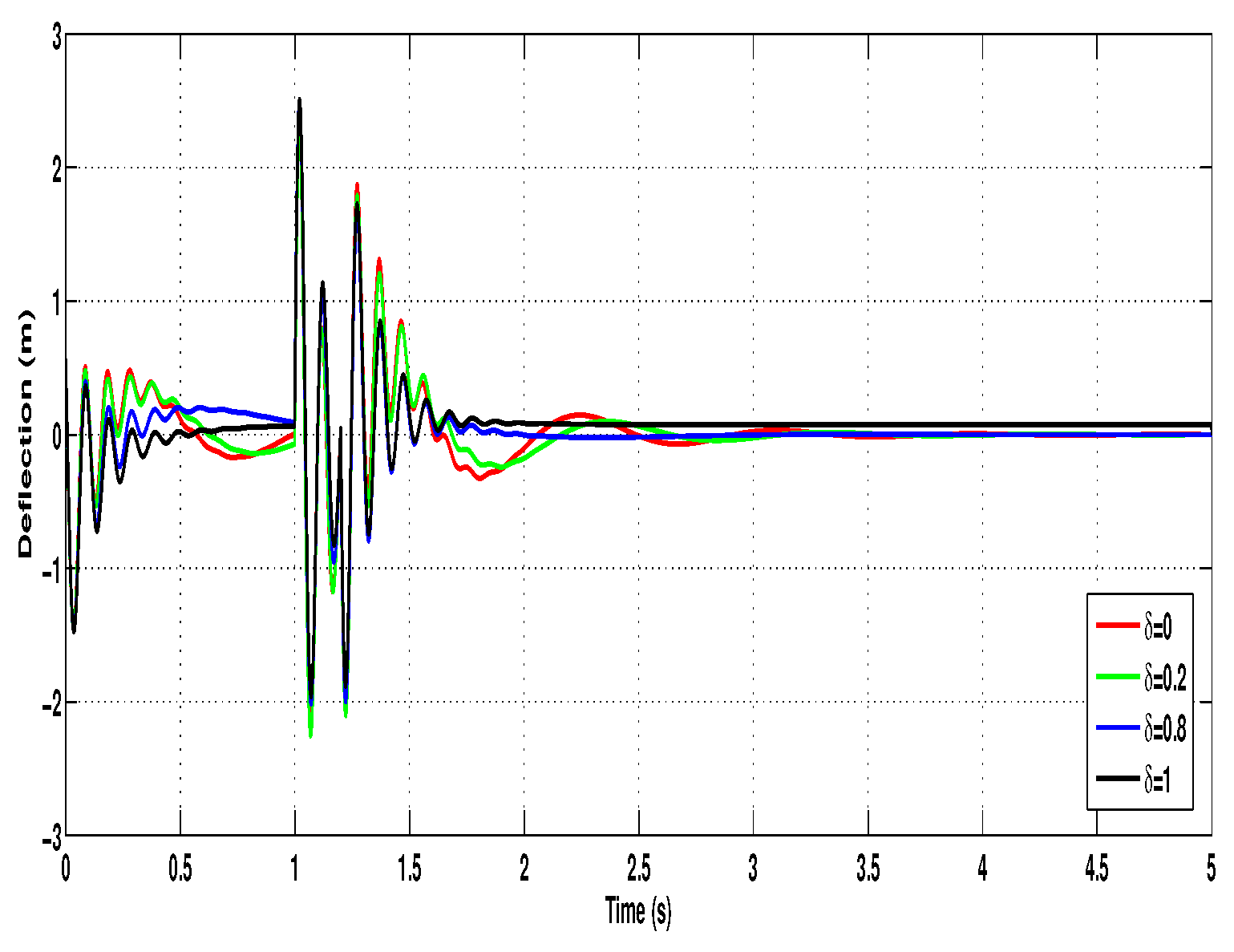
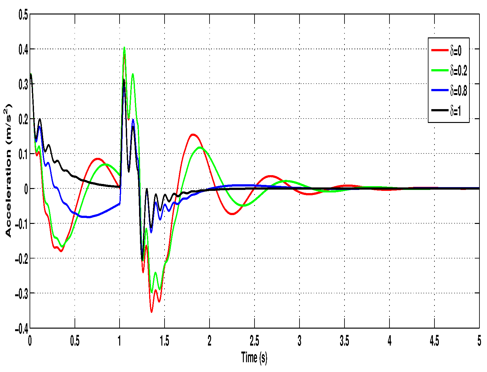
5.2. Fault Scenario Analysis
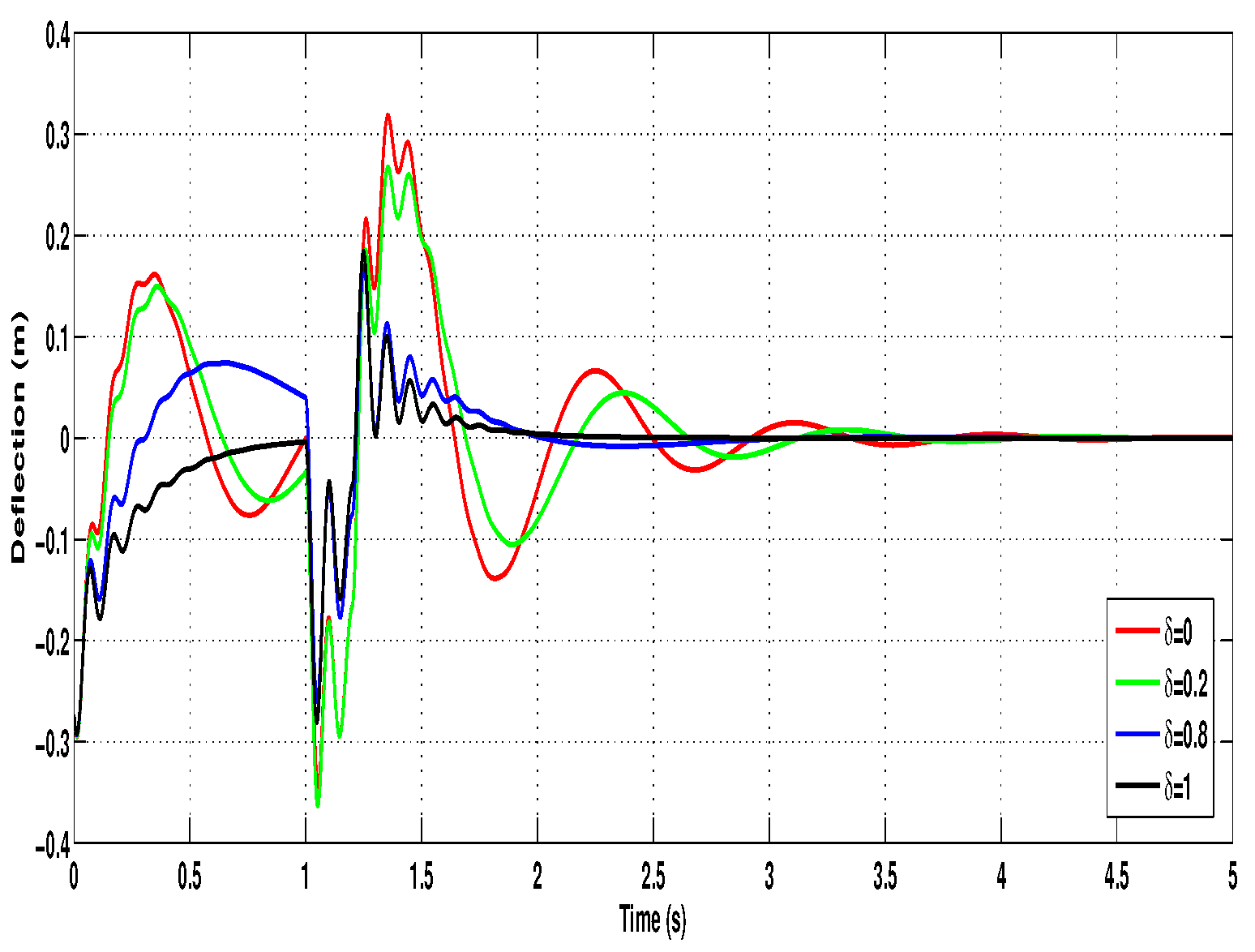
Finally, the impact of different levels of actuator faults on system behavior is investigated. The fault parameter is varied across four values:
- When , the actuator force becomes zero, effectively rendering the system a passive suspension system without any active control input;
- For and , the system experiences partial actuator faults, representing realistic scenarios where actuators lose effectiveness to varying degrees;
- When , the actuator operates with full effectiveness, corresponding to a fully healthy active suspension system.
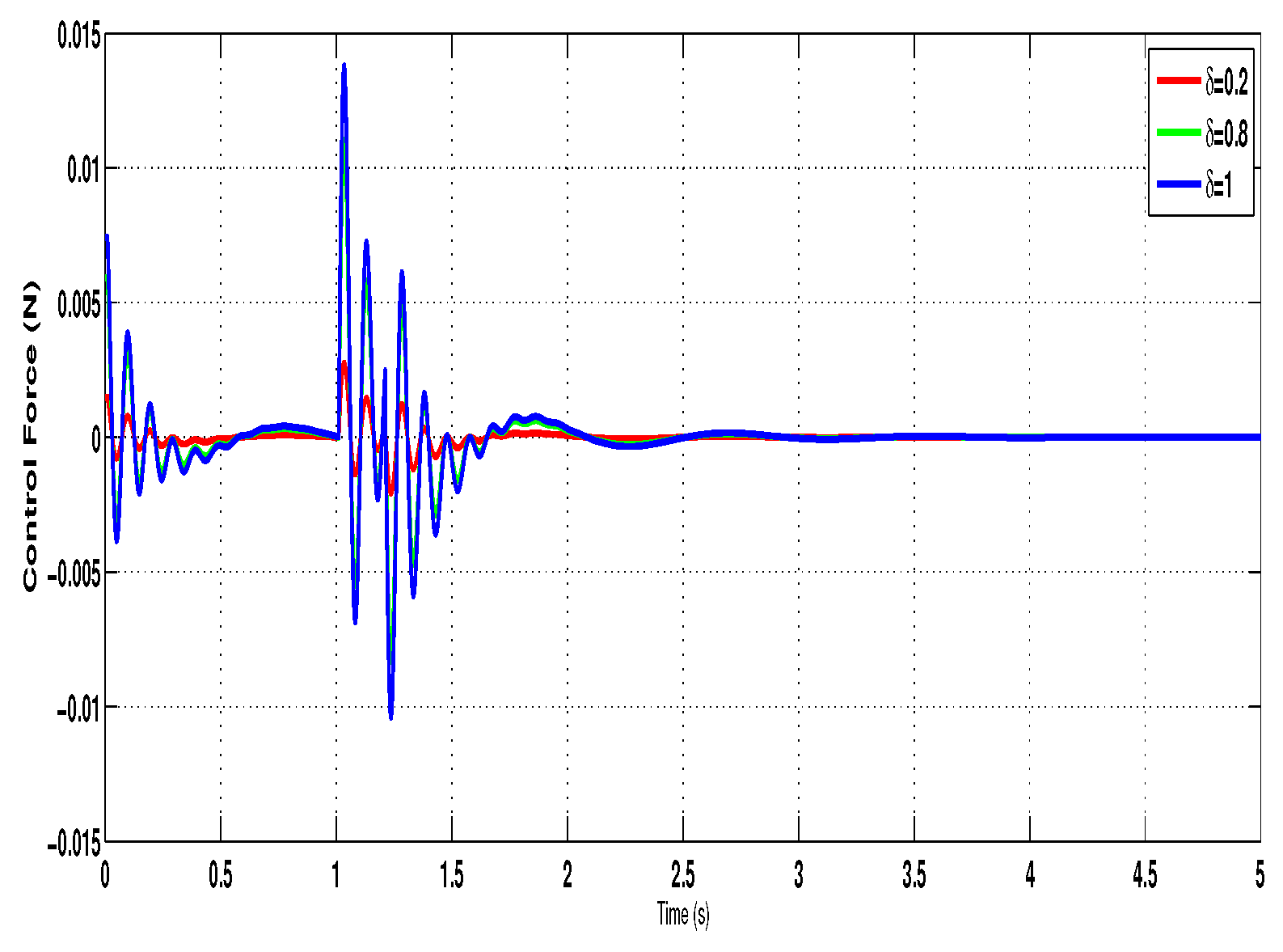
Figure 11, Figure 12 and Figure 13 display the output responses corresponding to each value. As expected, the passive system () exhibits reduced ride comfort and increased body displacement, highlighting the benefits of active suspension. Partial faults () introduce degraded but still stable performance, whereas the system maintains optimal performance in the case of a healthy actuator (). Additionally, the control input trajectories for , , and are plotted in Figure 14. The plots show that the control force magnitude adapts according to the fault severity, decreasing for lower values due to reduced actuator capability. Nevertheless, the system remains operational and stabilizes the vehicle body effectively under all fault scenarios, demonstrating the fault-tolerant nature of the proposed control scheme.
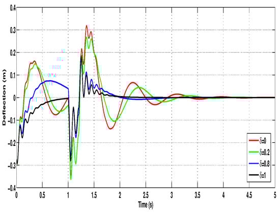
Figure 11.
Suspension deflection under different fault cases.
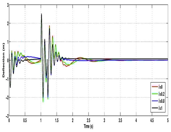
Figure 12.
Tire deflection under different fault cases.
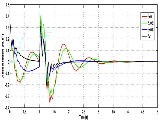
Figure 13.
Sprung mass acceleration under different fault cases.

Figure 14.
Control input under different fault cases.
6. Conclusions
This work has proposed a robust observer-based control framework for active EV suspensions that explicitly considers nonzero delays, actuator faults, and observer gain uncertainties. A novel dissipativity-based formulation was developed and integrated into an LMI framework to ensure stability and performance. The observer design enables reliable state estimation under perturbations, while the controller maintains the desired ride dynamics. The use of integral inequality techniques further reduces conservatism in the stability analysis. Simulation results confirms the approach’s effectiveness, showing rapid convergence and strongly fault-tolerant behavior. This framework offers a practical, resilient solution for advanced EV suspension systems.
Author Contributions
Conceptualization, A.S., R.R. and S.V.K.; Methodology, A.S. and R.R.; Software, A.S., J.A. and M.N.; Validation, A.S., R.R. and M.N.; Formal analysis, A.S., R.R. and M.N.; Investigation, A.S., J.A. and S.V.K.; Resources, J A., S.V.K. and M.N.; Data curation, A.S., J.A., S.V.K. and M.N.; Writing—original draft, A.S. and R.R.; Writing—review & editing, A.S., R.R., J.A., S.V.K. and M.N.; Visualization, J.A., S.V.K. and M.N.; Supervision, R.R.; Project administration, R.R.; Funding acquisition, J.A. and M.N. All authors have read and agreed to the published version of the manuscript.
Funding
This article was written with the joint partial financial support of RUSA Phase 2.0 Grant No. F 24–51/2014-U; Policy (TN Multi-Gen), Dept. of Edn. Govt. of India, PM-USHA Phase 3.0; DST-PURSE Phase 2 programme vide letter No. SR/PURSE Phase 2/38 (G); and DST (FIST-level I) 657876570 Grant No. SR/FIST/MS-I/2018/17.
Data Availability Statement
Data sharing is not applicable to this article as no new data were created or analyzed in this study.
Acknowledgments
J. Alzabut is thankful to Prince Sultan University for their help and support.
Conflicts of Interest
The authors declare that they have no conflicts of interest.
References
- Jin, X.; Wang, J.; Yang, J. Development of Robust Guaranteed Cost Mixed Control System for Active Suspension of In-Wheel-Drive Electric Vehicles. Math. Probl. Eng. 2022, 5, 4628539. [Google Scholar] [CrossRef]
- Shao, X.; Naghdy, F.; Du, H.; Li, H. Output feedback H∞ control for active suspension of in-wheel motor driven electric vehicle with control faults and input delay. ISA Trans. 2019, 92, 94–108. [Google Scholar] [CrossRef]
- Meng, Q.; Qian, C.; Sun, Z.-Y.; Chen, C.-C. A homogeneous domination output feedback control method for active suspension of intelligent electric vehicle. Nonlinear Dyn. 2021, 103, 1627–1644. [Google Scholar] [CrossRef]
- Jin, X.; Wang, J. Modeling and µ Synthesis Control for Active Suspension System of Electric Vehicle. In Proceedings of the 5th CAA International Conference on Vehicular Control and Intelligence (CVCI), Tianjin, China, 29–31 October 2021; pp. 1–6. [Google Scholar]
- Pang, H.; Liu, X.; Shang, Y.; Yao, R. A Hybrid Fault-Tolerant Control for Nonlinear Active Suspension Systems Subjected to Actuator Faults and Road Disturbances. Complexity 2020, 23, 1874212. [Google Scholar] [CrossRef]
- Xiong, J.; Chang, X.; Park, J.H.; Li, Z.-M. Nonfragile fault-tolerant control of suspension systems subject to input quantization and actuator fault. Int. J. Robust Nonlinear Control 2020, 30, 20–43. [Google Scholar] [CrossRef]
- Choi, H.D.; Ahn, C.K.; Lim, M.T.; Song, M.K. Dynamic output-feedback H∞ control for active half-vehicle suspension systems with time-varying input delay. Int. J. Control Syst. 2016, 14, 59–68. [Google Scholar] [CrossRef]
- Ji, G.; Li, S.; Feng, G.; Li, Z.; Shen, X. Time-delay compensation control and stability analysis of vehicle semi-active suspension systems. Mech. Syst. Signal Process. 2025, 228, 112414. [Google Scholar] [CrossRef]
- Mahmoodabadi, M.J.; Nejadkourki, N.; Ibrahim, M.Y. Optimal fuzzy robust state feedback control for a five DOF active suspension system. Results Control. Optim. 2024, 17, 2666–7207. [Google Scholar] [CrossRef]
- Wong, P.K.; Li, W.; Ma, X.; Yang, Z.; Wang, X.; Zhao, J. Adaptive event-triggered dynamic output feedback control for nonlinear active suspension systems based on interval type-2 fuzzy method. Mech. Syst. Signal Process. 2024, 212, 111280. [Google Scholar] [CrossRef]
- Zeng, Q.; Zhao, J. Dynamic event-triggered-based adaptive finite-time neural control for active suspension systems with displacement constraint. IEEE Trans. Neural Netw. Learn. Syst. 2024, 35, 4047–4057. [Google Scholar] [CrossRef]
- Mrazgua, J.; Tissir, E.H.; Ouahi, M.; Tadeo, F. Reliable H∞ fuzzy control for fault-tolerant actuator failures of active suspension system. IFAC J. Syst. Control 2024, 27, 100258. [Google Scholar] [CrossRef]
- Gao, X.; Du, Y.; Han, S.; Zhao, W.; Zhou, J.; Zhang, T.; Chen, C.L.P. Multi-agent reinforcement learning for vibration control of regenerative active suspension. Eng. Appl. Artif. Intell. 2025, 153, 110809. [Google Scholar] [CrossRef]
- Shen, Y.; Li, Z.; Tian, X.; Ji, K.; Yang, X. Vibration Suppression of the Vehicle Mechatronic ISD Suspension Using the Fractional-Order Biquadratic Electrical Network. Fractal Fract. 2025, 9, 106. [Google Scholar] [CrossRef]
- Li, H.; Li, Y.; Zhang, S.; Zhang, P.; Deng, Z.; Wang, L.; Sun, Y. Optimization of Suspension Damping in High-Temperature Superconducting Maglev Based on Combined Skyhook-Groundhook Control. IEEE Trans. Appl. Supercond. 2025, 35, 3600205. [Google Scholar] [CrossRef]
- Allotta, B.; Pugi, L.; Colla, V.; Bartolini, F.; Cangioli, F. Design and optimization of a semi-active suspension system for railway applications. J. Mod. Transp. 2011, 19, 223–232. [Google Scholar] [CrossRef]
- Stephen, A.; Cao, Y.; Raja, R.; Alzabut, J.; Niezabitowski, M.; Lim, C.P. Globally asymptotic stability and synchronization analysis of uncertain multi-agent systems with multiple time-varying delays and impulses. Int. J. Robust Nonlinear Control 2022, 32, 737–773. [Google Scholar]
- Stephen, A.; Raja, R.; Alzabut, J.; Zhu, Q.; Niezabitowski, M.; Bagdasar, O. Mixed Time-Delayed Nonlinear Multi-agent Dynamic Systems for Asymptotic Stability and Non-fragile Synchronization Criteria. Neural Process. Lett. 2022, 54, 43–74. [Google Scholar] [CrossRef]
- Ye, Z.; Ni, H.; Xu, Z.; Zhang, D. Sensor fault estimation of networked vehicle suspension system with deny-of-service attack. IET Intell. Transp. Syst. 2020, 14, 455–462. [Google Scholar] [CrossRef]
- Wang, K.; He, R.; Li, H.; Tang, J.; Liu, R.; Li, Y.; He, P. Observer-based control for active suspension system with time-varying delay and uncertainty. Adv. Mech. Eng. 2019, 11, 11–13. [Google Scholar] [CrossRef]
- Zhang, W.; Fan, X. Observer-based event-triggered control and application in active suspension vehicle systems. Syst. Sci. Control. Eng. 2022, 10, 282–288. [Google Scholar] [CrossRef]
- Parvizian, M.; Khandani, K.; Majd, V.J. An H∞ non-fragile observer-based adaptive sliding mode controller design for uncertain fractional-order nonlinear systems with time delay and input nonlinearity. Asian J. Control. 2019, 23, 423–431. [Google Scholar] [CrossRef]
- Stephen, A.; Raja, R.; Alzabut, J.; Zhu, Q.; Niezabitowski, M.; Lim, C.P. A Lyapunov–Krasovskii Functional Approach to Stability and Linear Feedback Synchronization Control for Nonlinear Multi-Agent Systems with Mixed Time Delays. Math. Probl. Eng. 2021, 1–20. [Google Scholar] [CrossRef]
- Choi, H.D.; Kim, S.-K. Delay-Dependent State-Feedback Dissipative Control for Suspension Systems With Constraints Using a Generalized Free-Weighting-Matrix Method. IEEE Access 2021, 9, 145573–145582. [Google Scholar] [CrossRef]
- Stephen, A.; Rajakopal, K.; Raja, R.; Srinidhi, A.; Thamilmaran, K.; Agarwal, R.P. Non-fragile reliable control for multi-agent systems with actuator faults using an improved L-K functional. Nonlinear Dyn. 2025, 113, 6645–6669. [Google Scholar] [CrossRef]
- Fang, F.; Ding, H.; Liu, Y.; Park, J.H. Fault tolerant sampled-data H∞ control for networked control systems with probabilistic time-varying delay. Inf. Sci. 2021, 544, 395–414. [Google Scholar] [CrossRef]
- Jin, X.; Wang, J.; Sun, S.; Li, S.; Yang, J.; Yan, Z. Design of Constrained Robust Controller for Active Suspension of In-Wheel-Drive Electric Vehicles. Mathematics 2021, 9, 249. [Google Scholar] [CrossRef]


Disclaimer/Publisher’s Note: The statements, opinions and data contained in all publications are solely those of the individual author(s) and contributor(s) and not of MDPI and/or the editor(s). MDPI and/or the editor(s) disclaim responsibility for any injury to people or property resulting from any ideas, methods, instructions or products referred to in the content. |
© 2025 by the authors. Licensee MDPI, Basel, Switzerland. This article is an open access article distributed under the terms and conditions of the Creative Commons Attribution (CC BY) license (https://creativecommons.org/licenses/by/4.0/).