Controlling of Multichannel Objects with Non-Square Transfer Function

Abstract

The control of multichannel objects is an independent section of cybernetics. Traditionally, objects are considered in which the number of inputs coincides with the number of outputs, but there are separate publications devoted to cases when the number of inputs does not coincide with the number of outputs. Even for this purpose, special terminology has been invented. If traditionally the mathematical model of an object is a square matrix transfer function, then in this case the term “non-square matrix transfer function” is used. This term is unsuccessful, as shown in this article, since it combines problems that are simplified in comparison with traditional ones, and problems that are, strictly speaking, unsolvable. This article demonstrates that an additional number of object inputs is not only not a problem, but also offers additional opportunities, while an excess number of outputs is an insurmountable problem: one can only abandon the problem of controlling redundant outputs. This situation should not be confused with the situation of the presence of additional outputs of sensors of the controlled variable or intermediate values, which also serve to simplify the solution of the problem and not to complicate it. If output signals are understood as independent output values that should be independently controlled, then the number of outputs should never exceed the number of inputs, although this situation can easily be confused with some other similar situations. This article also shows an example of how additional signals, sometimes mistakenly called additional outputs, can be used, and gives recommendations for various situations.

1. Introduction

The control of objects with multiple inputs and multiple outputs (MIMO) is relevant in robotics, transport, industry and science [1,2,3,4,5,6,7,8,9,10,11,12,13,14,15,16,17,18,19,20]. Often, an object has several operating parameters, which we will generally call output signals, as well as several possible ways to influence them, which we will call input signals. In addition, any object is also affected by uncontrolled and unmeasured influences, called disturbances.

In the scalar case, the signals in the object and in the system as a whole are described as functions of time, and Laplace transforms are used to describe the relationships between them in the form of equations and to calculate the regulator. Transfer functions are used to describe each element that transforms the signal, including for the mathematical model of the object and the regulator, i.e., the ratio of the output signals to the input signals in the Laplace transform domain. In the multidimensional case, the signals are described by column vectors and the transfer functions are described by matrices; all of this is also in the Laplace transform domain. In particular, the equation of the object in this case has the form

$$X(s)=\left[\begin{array}{c}{x}_1\left(s\right)\\ \dots \\ x_n\left(s\right)\end{array}\right]=\left[\begin{array}{ccc}{w}_{11}\left(s\right)& \dots & w_{1n}\left(s\right)\\ \dots & w_{ij}\left(s\right)& \dots \\ w_{n1}\left(s\right)& \dots & w_{nn}(s)\end{array}\right]\times \left[\begin{array}{c}{u}_1\left(s\right)\\ \dots \\ u_n\left(s\right)\end{array}\right]=W(s)U(s)$$

Here $X(s)$ is the output signal of the object in the form of a vector, that is, a set of output signals; $U\left(s\right)$ is similarly a vector of input signals, that is, a set of possible impacts on the object; and $W(s)$ is a matrix of the influences of the corresponding inputs on the corresponding outputs.

The task of controlling an object is to ensure that the vector of output signals of the object $X(s)$ becomes as close as possible to the vector of the task $V(s)$ that is fed to the input of the system.

To control the object, the control error is calculated $E(s)$, which is then converted into a control vector $U(s)$ using a regulator. In this case, the error calculator equation describes the corresponding number of subtractors:

$$E(s)=\left[\begin{array}{c}{e}_1\left(s\right)\\ \dots \\ e_n\left(s\right)\end{array}\right]=V(s)-X(s)=\left[\begin{array}{c}{v}_1(s)-x_1(s)\\ \dots \\ v_n(s)-x_n(s)\end{array}\right].$$

The controller equation is described through the product of the controller matrix transfer function $R(s)$ as follows:

$$U(s)=\left[\begin{array}{c}{u}_1\left(s\right)\\ \dots \\ u_n\left(s\right)\end{array}\right]=\left[\begin{array}{ccc}{r}_{11}\left(s\right)& \dots & r_{1n}\left(s\right)\\ \dots & r_{ij}\left(s\right)& \dots \\ r_{n1}\left(s\right)& \dots & r_{nn}\left(s\right)\end{array}\right]\times \left[\begin{array}{c}{e}_1\left(s\right)\\ \dots \\ e_n\left(s\right)\end{array}\right]=R(s)E(s).$$

It is natural to assume that the number of input values coincides with the number of output values, and therefore that the controller matrix and the object matrix are square matrices of dimension $n\times n$. The matrix $n\times m$ will not be square if the number of rows $n$ does not coincide with the number of columns $m$. For a matrix transfer function, the number of rows $n$ corresponds to the number of outputs, and the number of columns $m$ corresponds to the number of inputs of the element. The column vector of input signals is multiplied on the matrix transfer function from the right; it must have as many rows as there are columns in the transfer function, otherwise multiplication from the right is impossible.

Recently, speculative articles have begun to appear that discuss the control of an object described by a non-square matrix transfer function [11]. There have even been dissertations on this topic, where the problem of controlling such an object is put forward as extremely urgent, declared complex, and then, using examples taken out of context, it is supposedly successfully solved [12].

But in science, every statement must be proven, or at least confirmed. Control of a multichannel object is traditionally understood as autonomous control, that is, solving the problem of independent control of each output value of this object separately. If, for example, two output values are controlled, and the third output value is dependent on these two values, then this third value, of course, also changes, but this change is not controlled. If the problem is set as reducing three values to zero, and the third value is an algebraic sum of two other values or their derivatives, then, provided that these two values are equal to zero, the third value will also become equal to zero. In this case, only the appearance is created that all three values have been reduced to zero. In fact, only two values are reduced to zero by control methods, and the third value becomes zero automatically as a result of the successful control of these two main values. Concealing this fact by manipulating the equations does not make this result any more new, significant, or essential for science; it does not make this result any more of a proof of the possibility of control in the case when there are fewer input values than output values, that is, when the dimension of the vector $U(s)$ is less than the dimension of the vector $X(s)$ and the vector $V(s)$.

Let us denote the dimension of the vectors $X(s)$ and $V(s)$ by $n$, and the dimension of the vector $U(s)$ by $m$. Here $n$ is the number of outputs of the object and $m$ is the number of inputs of the object.

The standard situation is in the relation $n=m$. In this case, the matrices of the transfer functions of the object and the controller are square. The matrix transfer function of the object is not square if $n\ne m$. To declare the solution of the problem for the case of a non-square matrix transfer function of an object as a relevant research topic means to combine two fundamentally different cases.

The first case $n<m$ is not a problem, as this article will demonstrate. If $n=1$, the object is called MISO, which means that it has many inputs and a single output [13,14].

The second case, when $n>m$, does not provide the possibility of solving the problem in the form in which such a problem is traditionally understood. If in this case $m=1$, the object is called SIMO, which means that it has a single input and multiple outputs. Control traditionally involves ensuring that each of the output signals, which are called the outputs of the object, can be controlled independently of the other output signals. All other options are not control. But maintaining all deviations at zero is an easier task than autonomous control. For this reason, there are equilibrists who manage to maintain a structure with many degrees of freedom in equilibrium for some time, although in fact, when balancing, equilibrists use more than two degrees of freedom to control the balance. Indeed, it seems that an equilibrist can move a stand with a pyramid of cylinders only in two directions—forward–backward and right–left. In fact, the equilibrist also uses up–down movement, as well as a complex action in the form of movement along a short arc, for example, sharply forward–down and then forward–up, which has a stronger effect on the upper elements of the pyramid than on its lower elements. And even in this case, the equilibrist can only maintain balance for a short time and would not be able, for example, to return only one element to a state of equilibrium without disturbing the balance of the others, or to move some element to a new position without moving the other elements.

It should also be noted that even the traditional case, when $n=m$, is not always a solvable problem. It is advisable to distinguish the cases as follows: (a) cases where it is impossible to solve the problem in principle; (b) those with the impossibility of solving the problem in the class of static stationary solutions.

This article does not consider the issue of the solvability of the control problem in the case of a square matrix transfer function of an object; this issue is beyond the scope of the stated goals. However, we can briefly say the following.

There is no need to determine the rank of a square matrix when using numerical optimization methods: if the rank of a matrix transfer function coincides with its dimension, this is a necessary but not sufficient condition for the possibility of solving the stated problem of controlling such an object. The matrix of the transfer function may be singular: (a) in the strict sense of this concept; (b) in the static mode. The first option is extremely unlikely, since the matrix consists of functions and it will be singular in the strict sense of this formulation only if, for example, one of the rows is completely linearly dependent on the other rows in the entire frequency range. Option (b) is that this functional matrix may be singular in the region of zero frequencies. This is a more probable case, and it is not fatal—control of such an object is still possible—but this is a special case that is not considered in this article. Solving the problem using the numerical optimization method reveals all possible problems with an object that has a square matrix transfer function, including the problem that the rank of a square matrix will be less than its dimension.

But this article is not devoted to objects with a square matrix transfer function. The article is devoted to the problems of controlling objects with a non-square matrix transfer function. This article does not propose using, for example, the Riccati equation [21,22,23], which gives an expression for the controller matrix through the inverse matrix of the object. If this were applied, then the analysis of the rank of the square matrix would make sense. But this article does not invert the matrix transfer function of the object. This analytical method is also not used for the reason that it cannot be applied if the object model has a pure delay. In addition, if the number of inputs is greater than the number of outputs, analytical methods do not provide a method for using all the advantages of all the inputs of the object, they can only recommend ignoring the extra inputs. Such a method, apparently, can be developed for some special cases, but this is not relevant, since the numerical optimization technique successfully solves this problem, and it does not require a preliminary analysis of the rank of the functional matrix transfer function of the object and other complexities. Therefore, within the framework of this article there is no need to discuss the necessary conditions for the solvability of a problem if there is a method for checking and using sufficient conditions for its solvability.

2. Statement of the Problem

The task is to study the content of the problem of controlling objects with square and non-square matrix transfer functions using specific examples [1,2,3,4,5,6,7,8,9,10,11,12,13,14,15,16,17,18,19,20,24,25,26,27,28,29]. In this case, square matrix transfer functions are used only for comparison; the main goal of this study is precisely objects with a non-square matrix transfer function.

For this purpose, convincing justification and formulation of estimates of the complexity of the problem for the cases $n=m$, $n<m$ and $n>m$ are necessary.

3. The Method for Solving the Problem

Transfer functions are best suited for describing the mathematical model of a linear object, whereas the mathematical models of nonlinear objects are more adequate in the area of functions in the time domain rather than in the frequency domain. VisSim V5.0e software, which is best suited for the tasks of modeling and optimizing such systems, seamlessly uses both types of these mathematical models together, which facilitates its use for these purposes [30,31].

The apparatus of Laplace transfer functions, as well as Laplace–Carlson, and the Duhamel integral are widely used in analytical methods for calculating regulators and analyzing systems. The peculiarity of analytical methods is that they deal with analytical relationships, in particular with transfer functions, and use mathematical transformations of these relationships to obtain the desired result. These methods can currently be called obsolete when applied to problems of regulator synthesis. The reason for this is that regulators can only be designed using analytical methods for objects whose mathematical models do not contain pure delay links. If the object does contain pure delay links, then either they must be neglected or they must be approximated, for example, using the Padé approximation. In both cases, the result is unreliable and its use does not give the desired result. If the model of the object does not contain pure delay links, then, based on many theoretical and experimental studies, the author undertakes to assert that this model is insufficiently detailed. That is, such a model does not contain those details that most affect the correspondence of the calculation results with the results of applying this calculation in practice. Thus, analytical methods are either extremely complex, but at the same time not accurate enough or simply unsuitable. For this reason, this article does not consider analytical methods. For the same reason, we do not attempt an analytical approach, which preliminarily requires determining the rank of the matrix transfer function of the object. It is impossible to determine the rank of a matrix in general, but we can say for sure that the rank of a rectangular matrix is not greater than the smallest dimension of this matrix. This statement is sufficient for further theoretical reasoning.

The use of numerical modeling allows us to not only effectively calculate regulators for the most complex objects, but also to demonstrate the characteristic transient processes in the resulting system. An additional advantage of this software product is its adequacy, which consists of a fairly accurate match between the modeling result and the result of using the result in practice with real objects and real regulators, but this adequacy is achieved only if a number of modeling and numerical optimization rules are followed. These rules are quite simple, but for a successful solution to the problems of controlling multichannel objects, it is desirable to bring them together.

VisSim software (each versions) contains three optimization methods integrated into it to find the minimum of the objective function, and one more optimization method to find the zero of the objective function. We used only the minimum search, in which case the objective function is called the cost function or simply “Cost”. The Powell, Polak–Ribiere and Fletcher–Reeves methods were used. Many years of experience show that the Powell method always works better when solving regulator optimization problems. This is manifested in the fact that sometimes other methods do not demonstrate convergence, that is, the optimization procedure ends with a message that the optimization could not be performed since one of the quantities reached an unacceptably large value, that is, ${10}^{38}$.

The convergence of the numerical optimization procedure depends on many factors. First of all, there is a whole class of problems where convergence is fundamentally impossible. For example, the problem of optimizing a PID controller for a second-order plant without delay and the problem of finding a PI controller for a first-order plant without delay cannot have convergence. But if the plant model has a delay, and if the target functions recommended in this article are used, then convergence is most often ensured by using the Powell method for controller optimization. This method is one of three built-in methods in the VisSim program. The other two methods work slightly worse. The “procedure convergence” condition is not the only condition that ensures a good result. The procedure may converge, but the resulting solution will not satisfy the designer. In this case, the designer must change the optimization conditions. This may be an increase in the modeling time, a decrease in time discretization, a change in the weighting coefficients in the cost function, the introduction of additional terms in the cost function, or even a change in the controller structure. The arsenal of these methods constitutes the qualification and art of the designer. To present all these methods, it would be necessary to write a whole textbook. Such a textbook has been written and published by the author, but the issues considered in this article are not in it, since these are new results that have not been published anywhere before. Some issues are also discussed in detail in the articles [14,30,31].

4. Results of the Problem Consideration

In the case that $n=m$, we have a square matrix

$$W(s)=\left[\begin{array}{ccc}{w}_{11}\left(s\right)& \dots & w_{1n}\left(s\right)\\ \dots & w_{ij}\left(s\right)& \dots \\ w_{n1}\left(s\right)& \dots & w_{nn}\left(s\right)\end{array}\right].$$

The analytical solution to the control problem is given by the Riccati equation, which contains the inverted matrix of the object [21,22,23]. It is obvious from this that if the matrix is singular, it cannot be inverted. That is, a square matrix should not have proportional rows or proportional columns. Formally, the determinant of the matrix should be determined. If it is equal to zero, the matrix is singular. Consequently, in this case, the problem has no solution.

But this reasoning is too formal. Moreover, it is not suitable for the situation with a non-square matrix. Although in the case of a non-square matrix the reasoning can be reduced to simple mathematical reasoning: if the matrix is non-square, the rank of the matrix should be determined, and in this case the number of outputs that can be controlled is equal to the rank of this matrix. In this case, for example, if the matrix has dimensions $2\times 3$ or $3\times 2$, in any case the rank of such a matrix is not greater than 2, so in this case it will not be possible to control more than two output signals of the object, and even then only if it is possible in the specified matrix to select a non-singular matrix of dimension $2\times 2$.

Let us explain with examples.

4.1. Example 1

Let the matrix transfer function of the object have the following form:

$$W(s)=\left[\begin{array}{cc}{\displaystyle \frac{4}{1+3s}}& {\displaystyle \frac{3}{1+5s}}\\ {\displaystyle \frac{8}{1+3s}}& {\displaystyle \frac{6}{1+5s}}\end{array}\right]=\left[\begin{array}{cc}{w}_{11}\left(s\right)& w_{12}\left(s\right)\\ {2w}_{11}\left(s\right)& {2w}_{12}\left(s\right)\end{array}\right]$$

Let us write down what the column vector of output signals of such an object is equal to.

$$X(s)=W(s)U(s)=\left[\begin{array}{cc}{w}_{11}\left(s\right)& w_{12}\left(s\right)\\ {2w}_{11}\left(s\right)& {2w}_{12}\left(s\right)\end{array}\right]\times \left[\begin{array}{c}{u}_1\left(s\right)\\ u_2\left(s\right)\end{array}\right]=\left[\begin{array}{c}{x}_1\left(s\right)\\ {2x}_1\left(s\right)\end{array}\right]$$

Here

$$x_1(s)=w_{11}(s)u_1(s)+w_{12}(s)u_2(s),$$

$${x_2(s)=2x}_1(s)={2w}_{11}(s)u_1(s)+2w_{12}(s)u_2(s),$$

Thus, we obtain the key constraint:

$${x_2(s)=2x}_1(s)$$

In this case, autonomous control is impossible by any means; that is, it is impossible to obtain arbitrary different values for $x_1(s)$ and $x_2(s)$. These are not two independent values, but two strictly dependent values.

For example, a ship in the ocean can be moved arbitrarily in two coordinates, one of which sets the latitude and the other sets the longitude. But if the ship is in a riverbed, which can be conventionally represented as a winding line on the globe, then it can only move along this line, movement in latitude will also determine movement in longitude. Thus, the presence of a connection deprives the ability to control one of the output values; they both cannot change arbitrarily at the operator’s discretion. In this case, we also note the following property: if we control one output value, then the second output value will also change according to some pattern. For example, if we want to bring a ship to a certain port, then it is enough for us to move along the riverbed to this port. In this case, we will control both movement in latitude and movement in longitude. If we reformulate our requirement, which consists of moving the ship to the port, as corresponding movements in latitude and longitude, then we can mistakenly interpret the situation as if we were changing both the latitude and longitude of the ship’s location exactly as we should. But this is self-deception. In fact, we control a single coordinate of movement, the ship, and the other coordinate changes depending on the change in this coordinate and in accordance with the existing relationships between these coordinates. In this sense, we cannot claim that we have two quantities controlled by us. We have only one independently controlled quantity, and another quantity that we do not directly control as it changes in accordance with existing laws.

4.2. Example 2

Let the matrix transfer function of the object have the following form:

$$W(s)=\left[\begin{array}{cc}{\displaystyle \frac{4}{1+3s}}& {\displaystyle \frac{3}{1+5s}}\\ {\displaystyle \frac{8}{1+2s}}& {\displaystyle \frac{6}{1+4s}}\end{array}\right].$$

Strictly speaking, this matrix is not singular. Therefore, it is possible to control such an object. But here it is appropriate to introduce the term “statically singular matrix”, which describes the statement that when $s=0$ the determinant of this matrix is equal to zero, and its rank is equal to one, i.e., one less than its dimension:

$$detW(0)=0, rangW(0)=1.$$

That is, the matrix is $W(0)$ “statically singular”, which means that the matrix is singular in the static regime when $s=0$. Consequently, some standard equilibrium regimes cannot be achieved in this case. Namely, if it is required that the output values of the object described by such a matrix take some constant steady-state value, then this requirement cannot be met by static control; that is, the control vector cannot consist of constants such that they would ensure independent constant values of the output vector.

In other words, in the static (established equilibrium) case we have

$$X(0)=W(0)U(0)=\left[\begin{array}{cc}{w}_{11}\left(0\right)& w_{12}\left(0\right)\\ {2w}_{11}\left(0\right)& {2w}_{12}\left(0\right)\end{array}\right]\times \left[\begin{array}{c}{u}_1(0)\\ u_2(0)\end{array}\right]=\left[\begin{array}{c}{x}_1(0)\\ {2x}_1(0)\end{array}\right].$$

If the input signals are constant, then the output signals are strictly related:

$${x_2(0)=2x}_1(0).$$

But this does not mean that autonomous control of such an object is strictly impossible. Autonomous control is possible, but only at the price that the input signals must change over time even if the output signals are required to be constant. But constant change in control signals is not always possible; it is possible only in very rare cases, in exceptional cases.

For example, if we want to transfer a spaceship from one orbit to another, then we must give it acceleration, but after the ship is in the desired orbit and has the required speed, it will then move under the action of inertia and gravity. In a stationary orbit, control signals are not required; that is, the engines can and should be turned off. This situation does not require an effect on the object in a static mode. That is, the control signals in an equilibrium state are zero.

If we want, for example, to lift a load to a certain height, then we must not only apply force to the rope on which the load is suspended, but also maintain this force unchanged in the equilibrium state. This situation describes static control signals in the equilibrium static state of the object.

But the case under consideration is different in that we cannot achieve the required equilibrium state of the object in a static mode using constant control signals. In order for the object to remain in the desired equilibrium state, we need to ensure a constant change in at least one of the control signals. This is reminiscent of the statement from the book by mathematician Lewis Carroll, Through the Looking Glass, which says, “You have to run as fast as you can just to stay in the same place”. For example, if a load slides down an oiled rope at a certain constant speed, then in order for the load to remain in its place, it is necessary to lift the rope at exactly the same speed, that is, to wind it onto some reel. It is clear that such a situation is almost never satisfactory in the task of controlling an object.

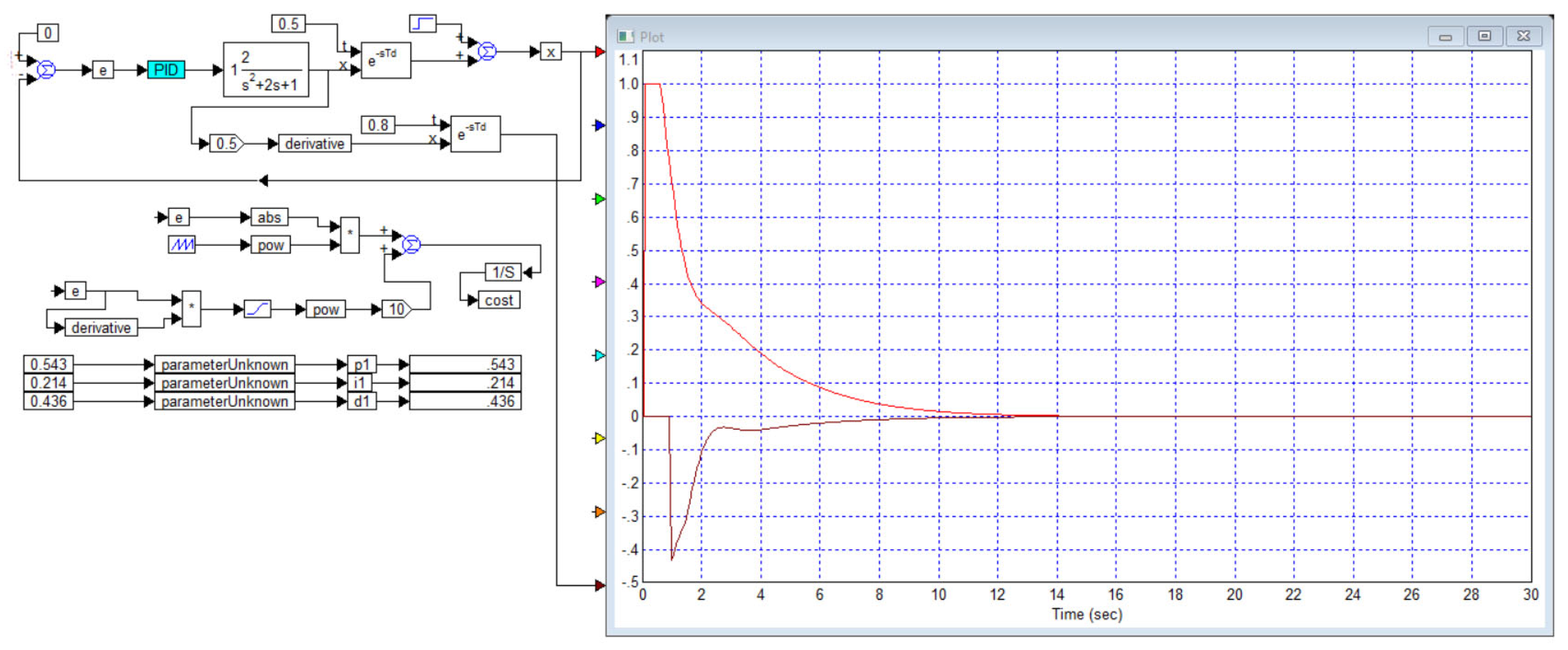
4.3. Example 3

Let us consider the problem of designing a controller for an object of dimension $2\times 2$ in the transfer function of which there are elements in the form of a third-order filter and a pure delay link connected in series with it.

$$W(s)=\left[\begin{array}{cc}{\displaystyle \frac{4}{1+s+s^2}}\mathrm{e}\mathrm{x}\mathrm{p}(-0.5s)& {\displaystyle \frac{3}{1+10s+10s^2}}\mathrm{e}\mathrm{x}\mathrm{p}(-0.5s)\\ {\displaystyle \frac{8}{1+2s+2s^2}}\mathrm{e}\mathrm{x}\mathrm{p}(-0.6s)& {\displaystyle \frac{6+6s}{1+10s+10s^2}}\mathrm{e}\mathrm{x}\mathrm{p}(-0.6s)\end{array}\right].$$

Here the delay link is described, as is traditional, in the Laplace transform domain by an exponential, in which the factor in front $s$ characterizes the delay time in seconds.

It is necessary to provide autonomous control of the object. The most common approach to solving this problem is to try to design a two-channel PID controller, the equation of which is as follows:

$$R(s)=\left[\begin{array}{cc}{P}_1+{\displaystyle \frac{I_1}{s}}+D_{1}s& P_2+{\displaystyle \frac{I_2}{s}}+D_{2}s\\ P_3+{\displaystyle \frac{I_3}{s}}+D_{3}s& P_4+{\displaystyle \frac{I_4}{s}}+D_{4}s\end{array}\right].$$

Different design methods consist of different ways of calculating the coefficients in this controller.

We propose a method of numerical optimization in the VisSim program Demo. In this case, a system is simulated, to which two different test signals are supplied:

$$v_1(t)=\sigma (t-2∆t)=\left\{\begin{array}{c}0,\forall t<2∆t\\ 1,\forall t\ge 2∆t\end{array}\right.,$$

$$v_2(t)=\sigma (t-0.5T)=\left\{\begin{array}{c}0,\forall t<0.5T\\ 1,\forall t\ge 0.5T\end{array}.\right.$$

Here $∆t$ is the discrete time step during modeling, $T$ is the modeling time and $\sigma (t-\tau )$ is a step function with a shift by a time interval $\tau .$

The cost function for optimization is calculated as the integral of two sums:

$$F(T)={\int }_0^T[{\sum }_{i=1}^2{e}_i(t)t^2+k_w{\sum }_{j=1}^2\mathrm{m}\mathrm{a}\mathrm{x}\{e_j(t){\displaystyle \frac{d{e}_j(t)}{dt}},0\}]dt.$$

Here $k_w$ is a positive weighting function, $e_i(t)=v_i(t)-x_i\left(t\right)$ is the error in each channel and a limiting function is used that zeroes out the negative component of the input signal, which is described by the following relationship:

$$\max \{A,0\}=\left\{\begin{array}{c}A,\forall A\ge 0\\ 0,\forall A<0\end{array}\right..$$

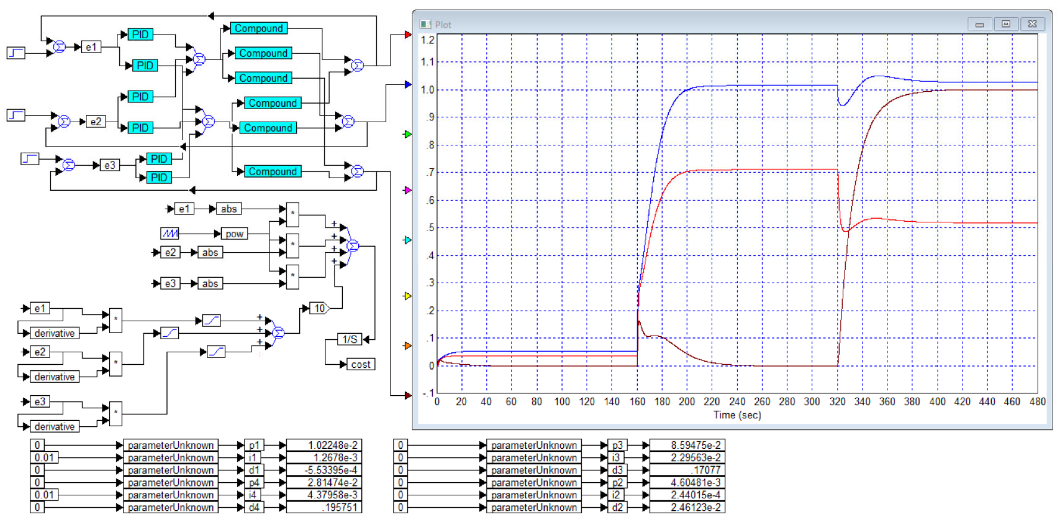
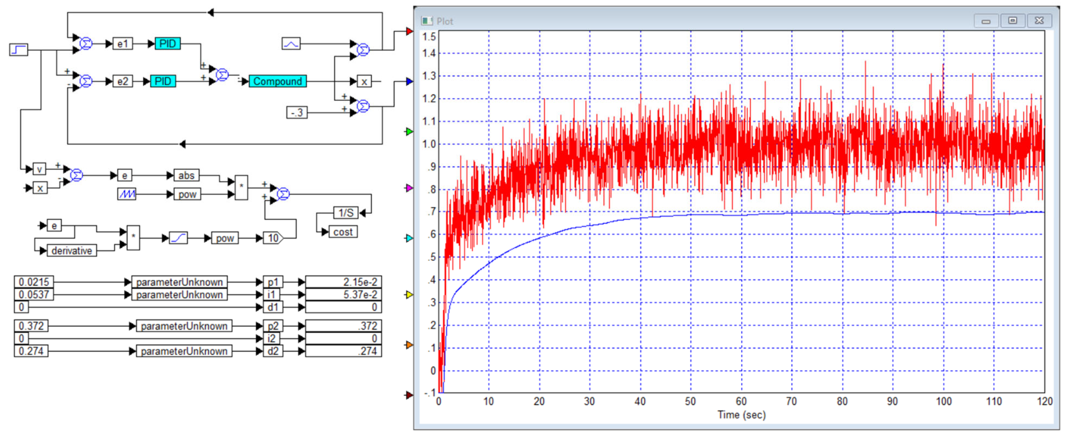
The project for optimizing the controller for this case using the specified method is shown in Figure 1. The resulting controller coefficients are recorded in the corresponding monitors. The resulting transient processes are shown on the oscilloscope on the right.

It is clear that we have partially succeeded in achieving separate control of the object, but this result is not yet actual autonomous control in the full sense of this meaning. If the task had been solved successfully, then the red beam would have reached a unit value quite quickly in accordance with the prescribed signal $v_1(t)$, and the blue beam would have shown a zero value for half the duration of the process, changing to a unit value at the moment $t=160 \mathrm{s}$. It is also highly desirable that these processes have minimal overshoot and minimal oscillation amplitude, and that these oscillations quickly damp out. The biggest problem in these processes is that the steady-state values do not coincide with the task.

However, these graphs show partial success in that the output signals are much closer to the setpoint (at the 80% level) and less dependent on the setpoint at the other input (at the level of no more than 25%). This result can be further developed by using more innovative approaches to controller design to bring this result to the desired one. However, the problem in this system is the shape of the control signals, the appearance of which is shown in Figure 2.

As we see, in order for the output signals of the object (and they are also the output signals of the system) to be approximately constant, it is necessary that the input signals of the object change at an approximately constant rate. But the input signals cannot increase or decrease indefinitely; therefore, in such a system it will not be possible to maintain constant prescribed levels for any length of time that would be independent of the tasks at other inputs. We propose to classify this as the impossibility of autonomy in a static mode with static control signals. The degeneracy of the object matrix in a static mode is the original problem to which one has to pay attention because in this case in practical it makes it impossible to solve the problem of the separate control of such objects.

If all the elements of the main diagonal of the transfer function of the object are much larger in absolute value than other elements in the matrix transfer function, this significantly simplifies the design of a multichannel controller. Even in the problem under consideration, when the matrix transfer function $s=0$ becomes stable, the predominance of diagonal elements can take place in the region of, for example, medium frequencies due to differentiating terms, which are manifested in the fact that the polynomial in the numerator has terms not only in the zero degree, but also in the first degree.

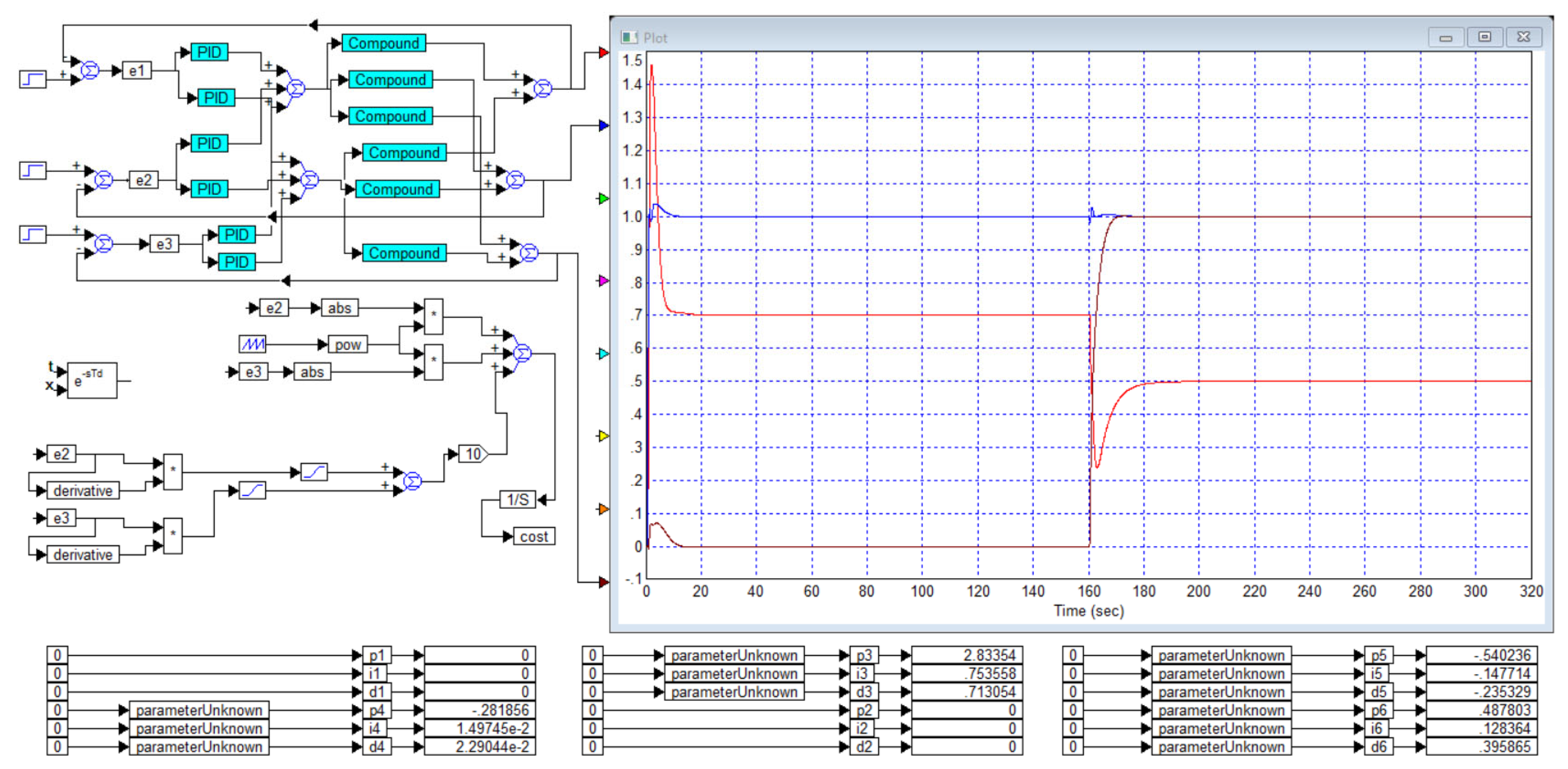
4.4. Example 4

Let us consider an object with a modified matrix transfer function:

$$W(s)=\left[\begin{array}{cc}{\displaystyle \frac{4+6s}{1+4s+4s^2}}\mathrm{e}\mathrm{x}\mathrm{p}(-0.5s)& {\displaystyle \frac{3}{1+10s+10s^2}}\mathrm{e}\mathrm{x}\mathrm{p}(-0.5s)\\ {\displaystyle \frac{8}{1+10s+10s^2}}\mathrm{e}\mathrm{x}\mathrm{p}(-0.6s)& {\displaystyle \frac{6+6s}{1+5s+5s^2}}\mathrm{e}\mathrm{x}\mathrm{p}(-0.6s)\end{array}\right]$$

In this transfer function the condition is preserved $detW(0)=0$.

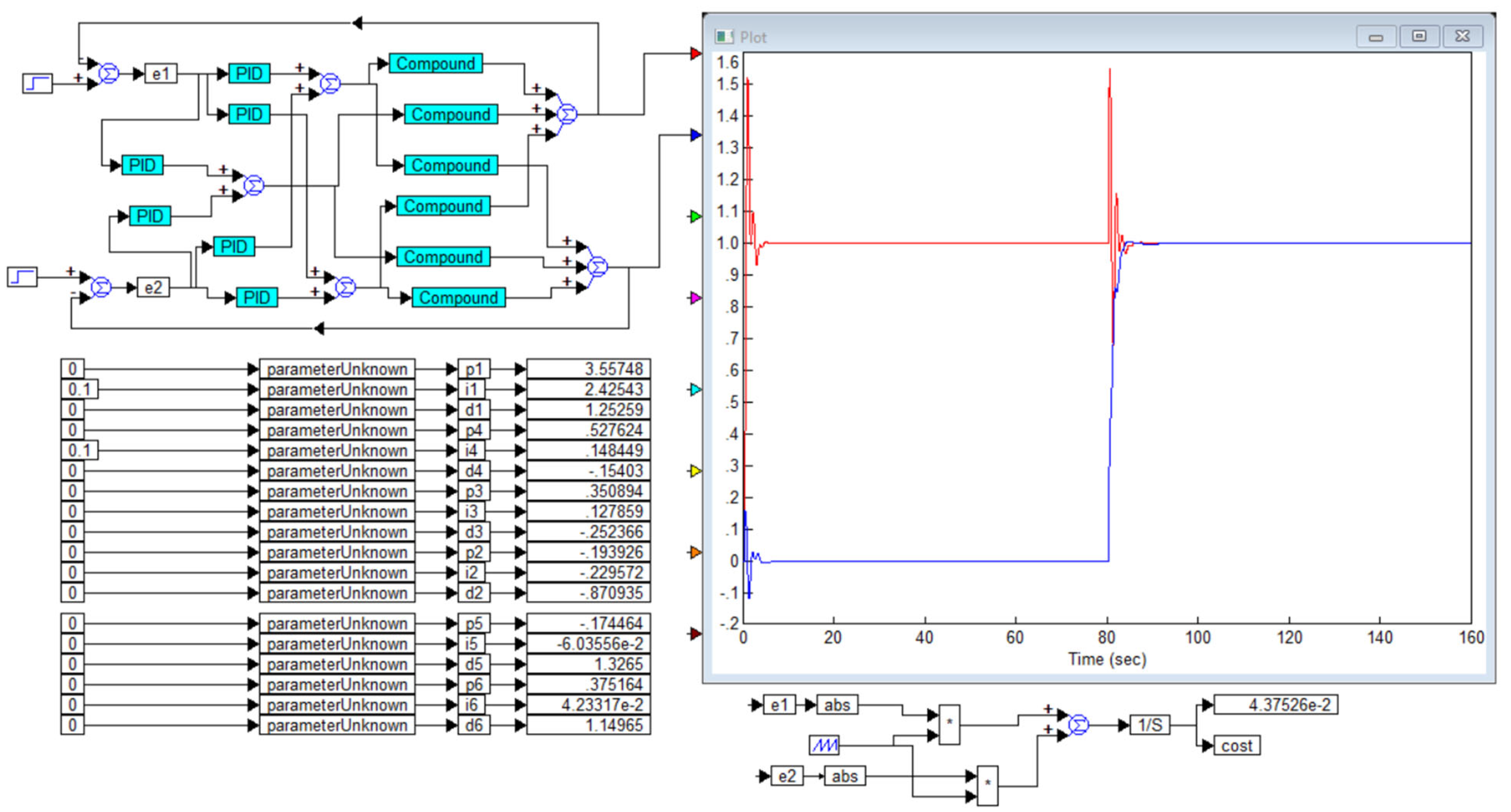
The numerical optimization method in this case also does not allow us to achieve the desired result. Figure 3 shows a project for optimizing a PID controller for such an object and it also shows the transient process in the resulting system, as well as the obtained controller coefficients. In this case, partial independent control is also achieved, but the control result remains insufficient, since in the second channel, instead of the zero equilibrium state, on the first interval of the process it takes a value of about 0.1 instead of the required zero value, and on the second interval it takes a value of about 0.96 instead of 1.0. In this case, it would also be possible to try to improve the result through innovative controller structures, but again a major problem with control signals would arise.

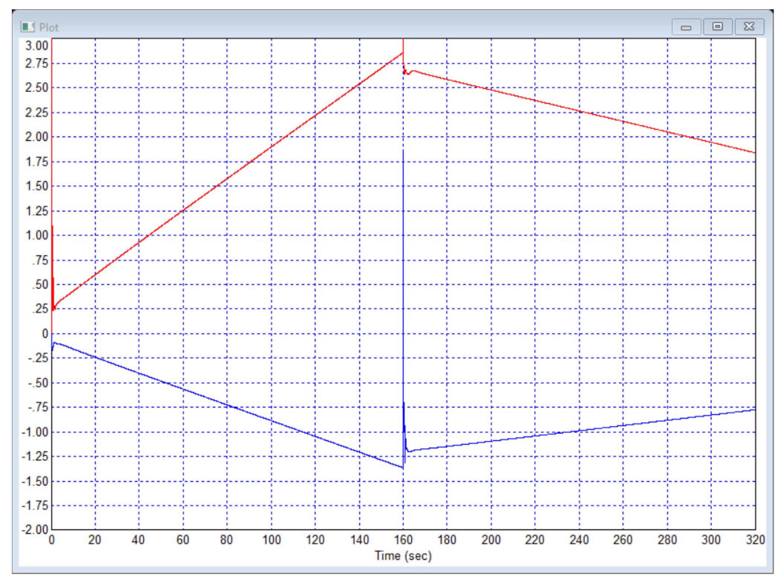
Figure 4 shows the type of control signals in this system. It is evident that these control signals do not tend to a constant equilibrium value over time but linearly increase or decrease in the section where the output signals are in an equilibrium state.

It is enough to at least slightly violate the property of “static degeneracy” of the matrix transfer function of the object, and its control becomes much easier after doing so.

4.5. Example 5

Let us consider an object with a modified matrix transfer function:

$$W(s)=\left[\begin{array}{cc}{\displaystyle \frac{6+4s}{1+4s+4s^2}}\mathrm{e}\mathrm{x}\mathrm{p}(-0.5s)& {\displaystyle \frac{3}{1+10s+10s^2}}\mathrm{e}\mathrm{x}\mathrm{p}(-0.5s)\\ {\displaystyle \frac{8}{1+10s+10s^2}}\mathrm{e}\mathrm{x}\mathrm{p}(-0.6s)& {\displaystyle \frac{6+6s}{1+5s+5s^2}}\mathrm{e}\mathrm{x}\mathrm{p}(-0.6s)\end{array}\right]$$

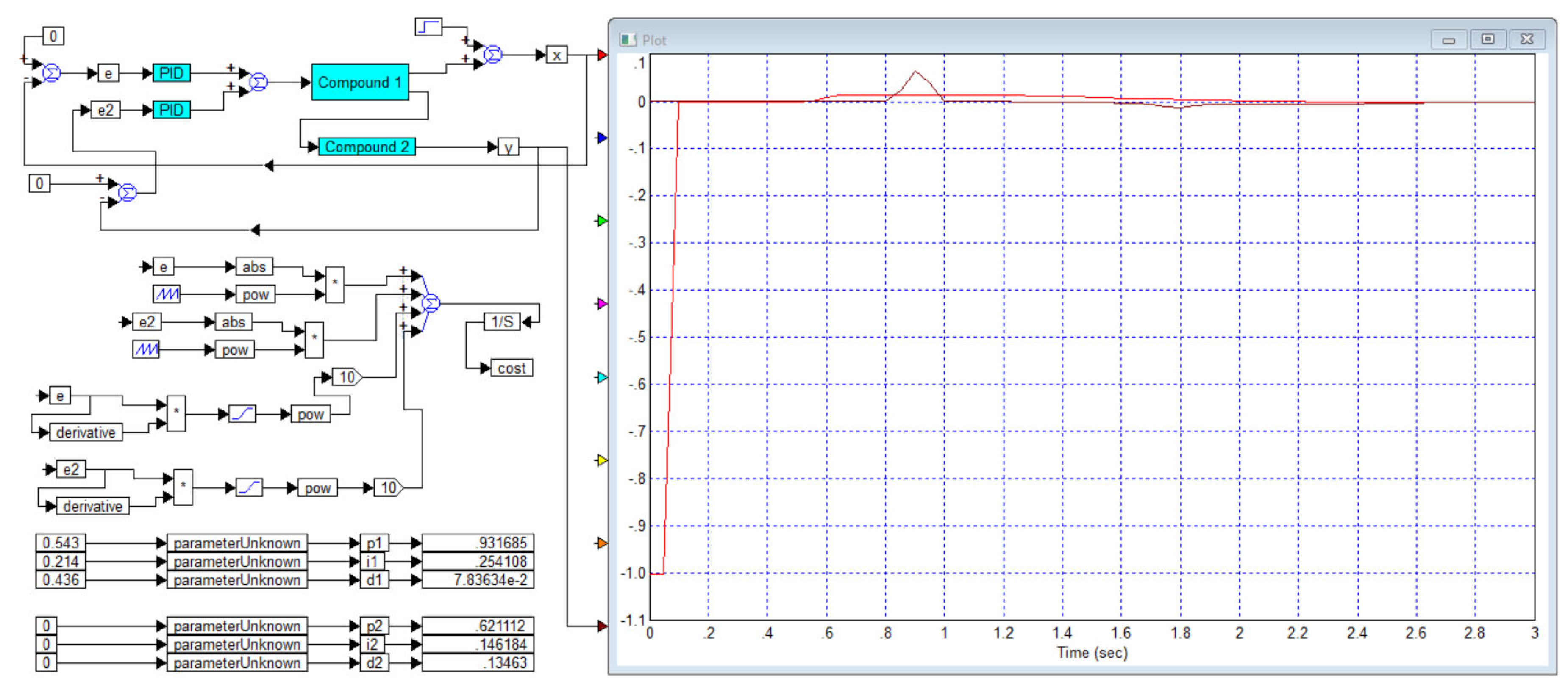
Here, in the upper left element in the numerator, in comparison with Example 4, the polynomial $4+6s$ is used instead of the $6+4s$ polynomial. This eliminates the static degeneracy of this matrix. The numerical optimization of the system with this object provides successful control. The project for optimization and the results are shown in Figure 5. In this Figure, after obtaining the exact values of the coefficients, they are all rounded to three significant digits, which ensures the result is checked for roughness. The system is rough, that is, no increased sensitivity to a negligible change in the coefficients are revealed, which proves the possibility of the practical application of the obtained result. Figure 6 shows the control signals in the system with these controller coefficients. These signals do not demonstrate a continuous increase in magnitude in those intervals where the output signals take the required values prescribed by the task signals. Therefore, the property of the obtained system is confirmed, consisting of the absence of the need for a constant increase or decrease in the control signals according to a law that is close to linear. This property, together with the sufficiently high quality achieved for the transient process, confirms the possibility of using the calculated regulator for the object of this example in practice.

This example demonstrates how undesirable the property of the static degeneracy of the object matrix is, and how much easier the task of controlling the object is if the matrix transfer function of the object does not have this undesirable property.

4.6. Example 6

Let us consider an object with a non-square matrix transfer function of dimension $2\times 3$, i.e., two rows and three columns:

$$W(s)=\left[\begin{array}{ccc}{\displaystyle \frac{2}{1+2s+s^2}}\mathrm{e}\mathrm{x}\mathrm{p}(-0.5s)& {\displaystyle \frac{3}{1+5s+s^2}}\mathrm{e}\mathrm{x}\mathrm{p}(-0.3s)& {\displaystyle \frac{0.5}{1+4s+2s^2}}\mathrm{e}\mathrm{x}\mathrm{p}(-0.7s)\\ {\displaystyle \frac{2}{1+6s+3s^2}}\mathrm{e}\mathrm{x}\mathrm{p}(-0.8s)& {\displaystyle \frac{4}{1+6s+{3s}^2}}\mathrm{e}\mathrm{x}\mathrm{p}(-0.3s)& {\displaystyle \frac{4}{1+4s+2.5s^2}}\mathrm{e}\mathrm{x}\mathrm{p}(-0.4s)\end{array}\right].$$

In this case, there are three inputs, each of which influences two outputs, and two output quantities that must be controlled.

Solving the problem of controlling such an object does not present any problem, if only for the reason that the developer can simply ignore any of the three inputs of the object. Mathematically, this means deleting any column in the given matrix. It is logical to delete the most undesirable column, that is, to leave two such columns, so that the resulting matrix would be, firstly, not degenerate even in its static version, and secondly, so that, if possible, the elements of the main diagonal would be greater in absolute value than the elements of the secondary diagonal.

But we will demonstrate that there is another way, which consists of using all three inputs and doing something extremely simple: calculating all the coefficients of such a regulator with a dimension $3\times 2$ using the numerical optimization method according to the procedure already demonstrated earlier.

Figure 7 shows the design and the results of optimization using a simplified cost function in which the last two terms are missing, namely

$$F(t)={\int }_0^T[{\sum }_{i=1}^2{e}_i(t)t^2]dt.$$

In this case, the problem is solved relatively successfully, except for the fact that there is significant overshoot in the processes, more than 50%. It is precisely to reduce overshoot that the last two terms in the cost function are intended.

Figure 8 shows the design and the result of controller optimization using the full cost function, into which the square root is additionally introduced according to the following relationship:

$$F(t)={\int }_0^T[{\sum }_{i=1}^2{e}_i(t)t^2+k_w\sqrt{{\sum }_{j=1}^2\mathrm{m}\mathrm{a}\mathrm{x}\{e_j(t){\displaystyle \frac{d{e}_j(t)}{dt}},0\}}]dt.$$

The introduction of the square root allows us to increase the influence of extremely small values on the cost function, which effectively suppresses not only the largest overshoot values but also small ones. In this case, the weight function $k_w=100$.

As can be seen from the result, in the second channel the overshoot is completely eliminated and in the first channel it does not exceed 10%. However, in this case, the duration of the transient process in the second channel is too long compared to the result shown in Figure 7. Therefore, it is advisable to try optimization with a smaller value of the weighting coefficient. Figure 9 shows the result using the value $k_w=10$.

This result is quite satisfactory. However, we will show that this solution is not the only possible one. In particular, we can swap the feedback; namely, instead of closing the feedback from the first output through the first input and replacing the feedback from the second output through the second input, we will try to do it differently. Figure 10 shows the project and the result when the signal from the first output of the object is fed into the subtractor at the second input of the system and the signal from the second output of the object is fed onto the subtractor of the first input of the system.

This is equivalent to a simple replacement of the numbering of the object outputs, and in this case the matrix transfer function of the object takes a new form:

$$W(s)=\left[\begin{array}{ccc}{\displaystyle \frac{2}{1+6s+3s^2}}\mathrm{e}\mathrm{x}\mathrm{p}(-0.8s)& {\displaystyle \frac{4}{1+6s+{3s}^2}}\mathrm{e}\mathrm{x}\mathrm{p}(-0.3s)& {\displaystyle \frac{4}{1+4s+2.5s^2}}\mathrm{e}\mathrm{x}\mathrm{p}(-0.4s)\\ {\displaystyle \frac{2}{1+2s+s^2}}\mathrm{e}\mathrm{x}\mathrm{p}(-0.5s)& {\displaystyle \frac{3}{1+5s+s^2}}\mathrm{e}\mathrm{x}\mathrm{p}(-0.3s)& {\displaystyle \frac{0.5}{1+4s+2s^2}}\mathrm{e}\mathrm{x}\mathrm{p}(-0.7s)\end{array}\right].$$

The numerical optimization project and its result for this case are shown in Figure 10. As we can see, this result is also quite satisfactory.

Overshoot in all channels does not exceed 3%. The application of this system is not at all more difficult, it is just that the second input of the system should now be used to control the first object output, and the first input of the system should be used to control the second object output.

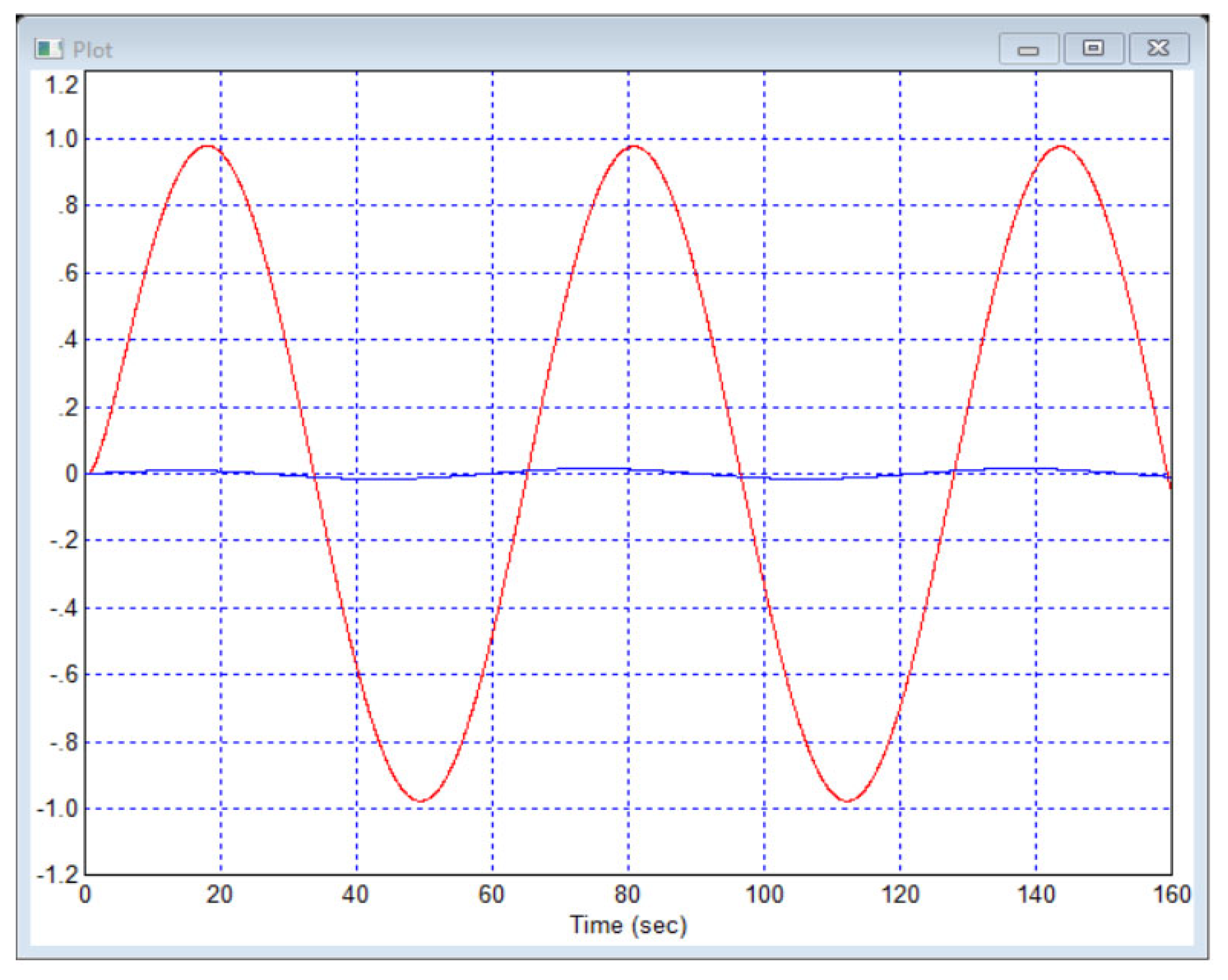
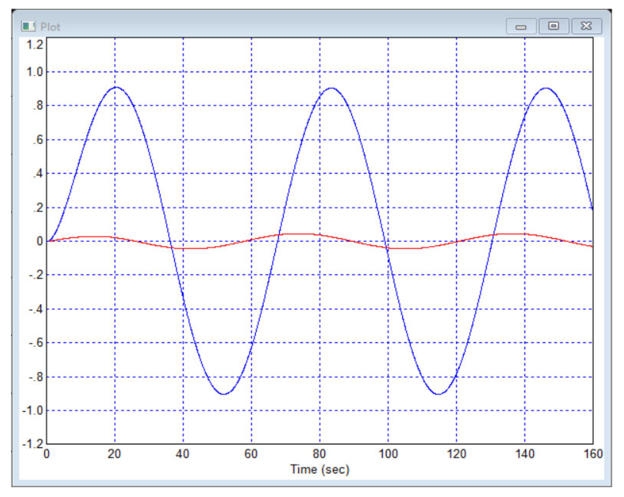
Figure 11 shows the system response to step interference of unit amplitude, which sequentially affects the first and second channels of the object. While the interference is applied to the outputs through a summing link, they are not filtered by the properties of the object. Figure 12 shows the output signals when a harmonic signal in antiphase is received at the inputs of the system. Figure 13 and Figure 14 show the output signals of the object when only one input is fed with a harmonic signal and the second input is fed with a zero reference signal.

Thus, as we see in the example, confirming the theoretical forecast, the additional inputs of the object are not a problem; they are, at least, an optional feature. If the developer prefers a method based on refusing to use one of the inputs of the object, it is recommended to give preference to those inputs that do not have nonlinearity, have a smaller delay or are not prone to oscillations. If the developer has difficulty choosing, they can either use the demonstrated method or alternately examine the result when refusing to use one of the inputs; that is, they can use one of three possible transfer functions:

$$W_1(s)=\left[\begin{array}{cc}{\displaystyle \frac{2}{1+2s+s^2}}\mathrm{e}\mathrm{x}\mathrm{p}(-0.5s)& {\displaystyle \frac{3}{1+5s+s^2}}\mathrm{e}\mathrm{x}\mathrm{p}(-0.3s)\\ {\displaystyle \frac{2}{1+6s+3s^2}}\mathrm{e}\mathrm{x}\mathrm{p}(-0.8s)& {\displaystyle \frac{4}{1+6s+{3s}^2}}\mathrm{e}\mathrm{x}\mathrm{p}(-0.3s)\end{array}\right].$$

$$W_2(s)=\left[\begin{array}{cc}{\displaystyle \frac{2}{1+2s+s^2}}\mathrm{e}\mathrm{x}\mathrm{p}(-0.5s)& {\displaystyle \frac{0.5}{1+4s+2s^2}}\mathrm{e}\mathrm{x}\mathrm{p}(-0.7s)\\ {\displaystyle \frac{2}{1+6s+3s^2}}\mathrm{e}\mathrm{x}\mathrm{p}(-0.8s)& {\displaystyle \frac{4}{1+4s+2.5s^2}}\mathrm{e}\mathrm{x}\mathrm{p}(-0.4s)\end{array}\right].$$

$$W_3(s)=\left[\begin{array}{cc}{\displaystyle \frac{3}{1+5s+s^2}}\mathrm{e}\mathrm{x}\mathrm{p}(-0.3s)& {\displaystyle \frac{0.5}{1+4s+2s^2}}\mathrm{e}\mathrm{x}\mathrm{p}(-0.7s)\\ {\displaystyle \frac{4}{1+6s+{3s}^2}}\mathrm{e}\mathrm{x}\mathrm{p}(-0.3s)& {\displaystyle \frac{4}{1+4s+2.5s^2}}\mathrm{e}\mathrm{x}\mathrm{p}(-0.4s)\end{array}\right].$$

In addition, it is possible to combine inputs. For example, to control the first output, you can use the first and second inputs of the object, to control the second output, you can use the second and third inputs of the object, and so on. In total, there are ten options: (a) Three options for using two inputs to control the first output, and three further options for each option for using two inputs to control the second output; this is nine options in total. (b) Three options with a refusal to use one of the inputs to control the first output while using all three inputs to control the second output, and three mirrored options with a refusal to use one of the inputs to control the second output, for a total of six options. (c) An option using all three outputs. This sums to a total of ten options.

When using only two channels, it should be taken into account that if the delays in one channel are small and they are large in the other channel, then the quality of the transient processes is determined by the channel with the worst delay, since it is not possible to ensure autonomous control if at least one of the channels cannot compensate for the influence of the other channel.

With regard to the possibility of controlling three outputs using two inputs, the forecast is negative in advance; however, to be convincing, it is necessary to demonstrate what a formal attempt to solve this problem leads to.

4.7. Example 7

Let us consider an object with a non-square matrix transfer function of dimension $3\times 2$, i.e., three rows and two columns, for which we simply transpose the matrix from Example 6:

$$W(s)=\left[\begin{array}{cc}{\displaystyle \frac{2}{1+2s+s^2}}\mathrm{e}\mathrm{x}\mathrm{p}(-0.5s)& {\displaystyle \frac{2}{1+6s+3s^2}}\mathrm{e}\mathrm{x}\mathrm{p}(-0.8s)\\ {\displaystyle \frac{3}{1+5s+s^2}}\mathrm{e}\mathrm{x}\mathrm{p}(-0.3s)& {\displaystyle \frac{4}{1+6s+{3s}^2}}\mathrm{e}\mathrm{x}\mathrm{p}(-0.3s)\\ {\displaystyle \frac{0.5}{1+4s+2s^2}}\mathrm{e}\mathrm{x}\mathrm{p}(-0.7s)& {\displaystyle \frac{4}{1+4s+2.5s^2}}\mathrm{e}\mathrm{x}\mathrm{p}(-0.4s)\end{array}\right].$$

If we do not take into account the theoretical statement about the impossibility of solving this problem, we should try to create a PID controller of the dimensions of the system design ($2\times 3$) and, having compiled the corresponding cost function, try to calculate the coefficients of this controller using the numerical optimization method.

The specified experiment was carried out, and its results are shown in Figure 15. It is possible to ignore the error on any of the three channels and set the goal of controlling only two output values. In this case, these two selected channels become fully controllable, but the remaining channel is not controllable; therefore, the output signal on it has an arbitrary form, such as will be obtained regardless of the prescription. Figure 16 shows the result when the third channel is ignored, Figure 17 shows the result with the second channel ignored and Figure 18 shows the result with the first channel ignored.

If the output of a channel is ignored, we cannot call it an “output”, because in the problem of controlling an object, the output is the signal that needs to be controlled. An output, the signal through which the system is not controlled, is not called an output in the theory of automatic control. It is simply a reference value available for measurement and nothing more. Therefore, any article that seriously discusses systems in which there are more outputs than inputs demonstrates either a lack of understanding of the essence of control by the authors, a deliberate ignorance of scientific approaches and scientific interpretation of the concept of “achieving a result” or authors who use their own unfounded terminology, meaning something completely different, different from the concept of controlling a multichannel object or an object with many inputs and many outputs.

For example, we can consider not only the output signal as such, but also its derivative, or even two derivatives—the first and the second. These signals are interconnected. Of course, if we can reduce the output signal to zero by means of feedback and maintain it in this state for some time, then automatically all the derivatives of this signal will also be equal to zero. On this basis, of course, we could claim that a single feedback allows us to reduce several signals to zero, but in this case this is not at all the control of many quantities. This is the control of a single quantity, and the derivatives of this quantity are not controlled, they take their corresponding values due to the value that the quantity itself takes.

4.8. Example 8

Let us consider an object whose control consists of reducing both of its output signals to zero, but only one input is available for influencing the object.

The object can be described by a non-square matrix transfer function of the following form:

$$W(s)=\left[\begin{array}{c}{\displaystyle \frac{2}{1+2s+s^2}}\mathrm{e}\mathrm{x}\mathrm{p}(-0.5s)\\ {\displaystyle \frac{s}{1+2s+s^2}}\mathrm{e}\mathrm{x}\mathrm{p}(-0.8s)\end{array}\right].$$

Nothing is fed to the input, i.e., the task is zero. A single-step effect is fed into the first output in the form of interference.

It is possible, without paying attention to the fact that the problem is formally unsolvable, to model the given conditions and find the best regulator of the dimension using numerical optimization methods $1\times 2$. Figure 19 shows a project for solving this problem and the optimization result.

As we can see, a solution is found; therefore, formally there are grounds to assert that, even in the case when the number of inputs is less than the number of outputs, it is possible to solve the problem. But this is only an apparent refutation of our assertion. In fact, the second output is not independent. Although formally it is a different function, this function is not independent of the function that describes the transfer function from the input to the first output. It differs only in the dynamic coefficient and delay. If the output of the first object is reduced to zero, then the output of the second object will also be reduced to zero. There are two factors at play here: firstly, the connection of the transfer functions from the input to the first output and from the input to the second output, and secondly, the fact that the requirement under the conditions of the problem is only to reduce the output signals to zero.

In this case, the second controller is not necessary. To prove this fact, we optimize a simpler system in which the second PID controller is missing but the objective function still includes both control “errors”. The result is shown in Figure 20.

We could ignore the error in the “control” of the second “output” of the object. We put these terms in quotes because there is, strictly speaking, no second output and no control of this second output. Let us show this. We simply control the first output in order to reduce the first output signal to zero, and we simply neglect the changes in the signal at the second “output”. The result is shown in Figure 21. In this case, we obtained an error that was larger in magnitude, but the second “output” the error, although larger in duration, was smaller in magnitude, only −0.42 in peak value versus −1.0 as a result of applying the cost function to both output signals. Thus, it is shown that the problem is solved automatically even if no attention is paid to the second output.

5. The Advisability of SIMO Systems in Exceptional Cases

Let us consider examples of the feasibility of controlling an object with two outputs and one input. Such a task is called SIMO, which means that the object has a single input and multiple outputs.

Usually, in automatic control tasks, an output signal is used that is considered by default to be measurable. But in practice, this is almost never the case; the output signal itself is not available as an electrical signal, it can only be measured using a sensor. There are no ideal sensors. Some sensors are characterized by high zero-level stability, but they have a limited frequency band. Other sensors, for example, may have a high level of additive high-frequency interference. Still other sensors may have a large zero-level offset.

Example 9

Consider an object whose output can only be measured by one of two types of imperfect sensors. Let one sensor have high-frequency noise and let the other sensor have a zero-level offset.

The mathematical model of the object is given in the form of a transfer function which has the form

$$W(s)=\left[{\displaystyle \frac{2}{1+2s+s^2}}\mathrm{e}\mathrm{x}\mathrm{p}(-0.5s)\right].$$

Gaussian noise with a variance of 0.1 is mixed into the output of the first sensor.

The offset of the second sensor is −0.3; that is, the output signal of the second sensor differs from the input value it measures by this value.

If only the first sensor is used, then the control result will have an excessively large noise component. If only the second sensor is used, then as a result of control the output value will be shifted upward by 0.3 units; that is, instead of the prescribed value equal to $v(t)=1$, a shifted value will be obtained at the output, equal to $x\left(t\right)\approx 1.3$.

The solution to this problem is to use the output of each sensor, optimizing the controller so that the actual output signal of the object would be as close as possible to the task; that is, as an error during optimization, we calculate and use the true error of the output value. To simplify the problem, in the PID controller using the output of the noisy sensor, that is, the first output, we will not use the channel with the derivative and we will set this coefficient to be equal to zero by default. In the second PID controller, we will set the integrator coefficient to be equal to zero since this connection will obviously work incorrectly. The constant offset is especially sensitive to the integrator input.

Figure 22 shows the result of optimization in this case. Figure 23 shows the true output signal of the object, regardless of the shortcomings of each individual sensor. This output signal has neither offset nor significant noise.

6. Discussion

Based on the theoretical discussion and the experiments with numerical modeling, a general classification of the problems of controlling multichannel objects can be given.

The following options can be distinguished in the classification:

• A square matrix, non-singular for $s=0$. This is the most typical situation, since most researchers simply do not consider other variants of MIMO systems. This problem has a chance of being solvable. It is impossible to claim that it is necessarily solvable, since the solution of the problem may be hampered by negative coefficients in the polynomials of the denominators of individual transfer functions, as well as some insurmountable types of nonlinearities and other problems. In practice, insurmountable problems are rare, and sometimes problems that seem insurmountable can be overcome by using smart structures of regulators, but this is not the topic of this article.
• A square matrix, degenerate at $s=0$ but not degenerate at $s\ne 0$. This is the most atypical situation, but in principle, control of such an object is possible, although there are many features and the result may not satisfy the developer because the control signals do not remain stationary with a stationary assignment. This problem may be solvable, as in Example 4, but most often this turns out to be too high a price for controlling the object. Such problems can be called conditionally solvable.
• A non-square matrix of “more inputs than outputs”, MITO. This situation makes the object easier to control. Such a problem is almost always solved, or at least it has a higher chance of being solvable as it is much simpler than the previous two [14].
• Non-square matrix of “fewer inputs than outputs”, FITO. This problem is unsolvable in the formulation in which it is posed.
  • The outputs are not connected by a dependency relationship. This situation does not allow for the full control of the object: it is necessary to abandon the task of controlling excess outputs; it is possible to control the number of outputs that are equal to the number of inputs, provided that the corresponding matrix transfer function is not degenerate. The developer will come to an obvious failure.
  • The outputs are related by a dependency relation; for example, they are derivatives, integrals or other results of the dynamic transformation of other outputs. In this case, it is possible to simulate control in some special cases, for example, in the case of reducing the initial conditions to an equilibrium state in which all or many output signals must be equal to zero. The developer may mistakenly believe that the problem is solved, but this is a misconception, since it is not possible to achieve the stabilization of all the output values but only such a number of them as is equal to the number of inputs; the behavior of the remaining output signals is not controllable.
• A non-square matrix with more outputs than inputs, provided that the extra outputs are actually the outputs of other sensors that measure the same output values as the object but in a different frequency range or with different sensor properties, such as the presence or absence of various noises, drifts, constant offset, etc. In this case, we should not talk about extra outputs but about additional possibilities of measuring the same outputs. This situation can also be assessed as additional possibilities; it does not represent a difficulty. This problem is solvable, and its successful solution will provide a better result than ignoring signals from additional sensors. This situation is described in the literature [30].

In addition, this article demonstrated in detail how the numerical optimization algorithm works in practice, for example, in the case of using the VisSim program, and also provided explanations, illustrated with examples, of what modifications of the cost function (the objective function during optimization) are advisable to use—what test signals of the task—and how to make sure that the resulting system is rough (which allows it to be used in practice).

Regarding the convergence of optimization algorithms, the following can be stated. Zero-order algorithms work more reliably than first-order algorithms, i.e., algorithms that use the derivative of the objective function with respect to the arguments. To determine the full derivative, it is necessary to determine all partial derivatives with respect to all arguments, which requires trial tests in the amount equal to the number of arguments of the cost function. As a result, it is possible to obtain a gradient vector associated with the direction and magnitude of the greatest decrease in the cost function. Obviously, moving in the direction of this vector would be the best solution. But in this problem, this method is ineffective, firstly because it will require many tests just to determine the point of the next test, which is nonsensical. Zero-order methods allow one to directly calculate the point of a new test from a previously obtained set of tests, i.e., the full coordinates of the points in the space of the parameters being optimized and the values of the cost functions at these points. As we approach the minimum point, the gradient method becomes less and less effective, since the gradient value becomes smaller and smaller, and possible noise and calculation errors become increasingly significant hindrances compared to the gradient value. In addition, when the objective function is given as an analytical dependence in the form of an integral, then calculating the gradient is easier than calculating the cost function since the gradient is a derivative of the integral, that is, an integrand. But in our problem, there is no analytical expression for the dependence of the cost function on the arguments. The cost function is an integral of the error, and the error is not associated with any analytical explicit dependence on the controller parameters, it is only indirectly related, very indirectly, and this connection cannot be expressed by any known analytical relationship. If such a relationship existed, then numerical methods would not be required; the problem could be solved analytically.

The designer does not have to decide whether the algorithm converges or not. If the algorithm is stable, then after a certain number of tests the desired minimum point of the cost function will be found, and as a result the designer will know the desired regulator coefficients. If the algorithm is not stable, then the other two algorithms can be tried. But experience shows that the Powell algorithm works best, so it is recommended to start with it, and that using other algorithms is inappropriate. It is better to use one of the following approaches:

Modify the cost function by adding additional terms to it.

Increase the simulation time.

The cost function must meet the following requirements.

-

Dependence on all parameters: It must depend on all optimized parameters, at least indirectly.

-

Justification: It should take on the corresponding minimum value precisely when the requirements imposed on the system are achieved to the best degree.

-

The absence of point (awl-shaped) dips or peaks: Any smooth function satisfies this requirement (this is the name of a function that has continuous derivatives at all points), but this is not necessary. It is enough for the derivative to be finite; even the non-coincidence of the derivative on the left and the derivative on the right at one point is acceptable: this will lead to a sharp break in this function, which is acceptable. Even if the derivative is not finite, optimization may be possible if the second derivative is finite.

-

For the VisSim program it is necessary that the cost function be positive and bounded: $0<F(T)<{10}^{38}$.

The most effective way to ensure stability and the rapid attenuation of errors in the system is to use a term in the cost function proportional to the integral of the error modulus multiplied by the time from the start of the transient process. For even greater efficiency of this term, the error modulus can be used under the root and/or the time can be squared. It is also possible to increase the weighting coefficient before this term or decrease the weighting coefficients before all the other terms.

The most effective way to suppress overshoot, as well as inverse overshoot and the non-monotonicity of the transient process, is to use a term based on the integral of the positive part of the product of the error and its derivative. For greater efficiency in this term, this positive part can be taken under the root or the weight coefficient before this term can be increased.

The requirements of high speed (i.e., rapid error reduction) and low overshoot are in conflict, so the designer has to find a compromise solution that ensures the fulfillment of both these requirements.

For this reason, the task of designing a regulator is a task of double optimization: first, the coefficients are optimized according to the cost function proposed by the designer; second, the mathematical expression, weight coefficients and simulation time are also optimized to obtain the best solution, but this optimization is performed by the designer based on a visual assessment of the transient process graphs. After each change in at least one parameter of the cost function, the developer starts the automatic optimization procedure, and the obtained result is compared with the previously obtained results, for which it is recommended to save the sets of obtained coefficients. This allows the designer to simultaneously obtain several transient processes on the graph and select the best one, or to decide how to further change the cost function to obtain the best transient process.

There are situations when even with very significant changes in the cost function, the resulting system remains almost the same, which is evident from the values of the obtained regulator coefficients and from the type of the obtained transient process. This indicates that it is impossible to find a better solution with this regulator structure. In this case, you should either put up with the result, if it is satisfactory, or try to use another, more complex regulator structure. Such more-complex structures include, for example, two-loop systems. In this case, an object with a regulator is considered as a new object, the coefficients of this regulator are fixed, and a new external loop with negative feedback and a new sequential regulator is created around this new object. This method is quite effective in controlling SISO scalar objects; there are no examples of its use with multichannel MIMO objects in the literature, but at the current stage of development of software and hardware control tools, such a system is not unrealizable; it has the right to exist, at least for objects with two inputs and two outputs.

7. Conclusions and Findings

This article comprehensively studies the problem of the control of multichannel objects and pays special attention to situations where the number of inputs and the number of outputs do not match. Such cases, which are also sometimes called in the literature situation with a non-square matrix transfer function of the object, are considered in many articles, but a unified classification of all such situations based on the solvability of such control problems cannot be found in the literature. For this reason, there is erroneous interpretation and unfounded speculation in this area.

Experience has shown that the theoretical refutation of such erroneous statements as, for example, the statement about the possibility of controlling $m$ outputs using $n$ inputs under the condition $m>n$ is not enough; illustrative examples and extremely clear reasoning based on logic and mathematics are required. For example, it is obvious that the statement “a straight line can always be drawn through any three points” would be incorrect. Examples of three points through which a straight line can be drawn can also be given. But this statement is erroneous. A straight line can be drawn only through three points lying on the same straight line. In exactly the same way, the statement that it is possible to control an object that has more outputs than inputs is incorrect, although it is possible to invent and give examples of how it is possible to artificially (erroneously or intentionally) invent examples of such objects, using which it is possible to demonstrate something that outwardly resembles control, especially if the control consists of the task of reducing all output values to zero. From a theoretical point of view, this is equivalent to the statement that it is possible to find $n$ unknown values from any equations $m$ under the condition $m>n$. But this is not true. It is possible to find $m$ unknown values from $m$ equations. Here we do not discuss special cases where this is violated, such as when some equations are linear combinations of other equations. We argue that if there are more equations than quantities, then, in general, it is impossible to find all the quantities for which all the equations will hold, since there are more equations than quantities. Likewise, if there are fewer equations than quantities, then it is possible to find many variants or combinations of quantities for which all these equations will hold. This theoretical statement may be incomprehensible to some students and even some scientists, but it is easier to explain and prove with examples.

The theoretical statements presented here are formulated and published for the first time, since the author not only failed to find anything similar in the literature, but, on the contrary, can confirm with references the fact that there are incorrect classifications of objects as “objects with a non-square matrix function” and that articles have been written and successfully published on this topic, which would be equivalent to developing a direction in mathematics related to solving systems of equations in which the number of unknown quantities does not coincide with the number of equations.

Thus, this article aims to clarify the typical mistakes of many authors; this is its contribution and novelty, based on the proposed theoretical statements.

This article, based on theory and supported by practical examples, provides a well-founded classification of such situations.

The article also substantiates and demonstrates the need to check the obtained solutions for correctness. This check consists of the fact that all regulator coefficients obtained as a result of numerical optimization must necessarily be rounded to three significant digits, after which the system is re-simulated. The resulting transient processes in this case should not differ significantly from those processes obtained by the numerical optimization method.

This article does not consider the adaptive control method, but some results in this area have been obtained previously. In particular, one effective method is to change the gain of the controller according to the harmonic law with subsequent synchronous detection of the control error. This method, as it turns out, even by itself increases the stability of the system, and the feedback changing this coefficient additionally increases the stability of the system. This method was successfully tested on a single-channel SISO system, it can apparently be extended to control problems with multichannel objects in MIMO systems.

The author is extremely grateful to the reviewers for their valuable comments that helped improve this article.