Bi-Objective Optimization for Scalable Resource Scheduling in Dense IoT Deployments via 5G Network Slicing Using NSGA-II

Abstract

The proliferation of Internet of Things (IoT) devices demands efficient resource management in fifth-generation (5G) networks, particularly through network slicing mechanisms supporting massive machine-type communications (mMTCs). This paper addresses IoT connectivity in 5G network slicing through a bi-objective optimization framework balancing operational costs with quality-of-service. We formulate a bi-objective optimization problem that balances operational costs with quality-of-service (QoS) requirements across heterogeneous 5G network slices. The proposed approach employs a tailored Non-dominated Sorting Genetic Algorithm II (NSGA-II) incorporating domain-specific constraints, including device priorities, slicing isolation requirements, radio resource limitations, and battery capacity. Through extensive simulations on scenarios with up to 5000 devices, our method generates diverse Pareto-optimal solutions achieving hypervolume improvements of 8–13% over multi-objective DRL, 15–28% over single-objective DRL baselines, and 22–41% over heuristic approaches while maintaining computational scalability suitable for real-time network management (sub-2 min execution). Validation with real-world traffic traces from operational deployments confirms algorithm robustness under realistic burstiness and temporal patterns, with 7% performance degradation vs. synthetic traffic—within expected simulation–reality gaps. This work provides a practical framework for IoT resource scheduling in current 5G and future Beyond-5G (B5G) telecommunications infrastructures, validated in scenarios of up to 5000 devices.

1. Introduction

The exponential growth of Internet of Things (IoT) devices, projected to reach approximately 29 billion by 2030 [1], poses major challenges for mobile network architectures in terms of scalability, resource efficiency, and quality-of-service (QoS) assurance. To address these challenges, 5G networks introduced network slicing as a fundamental architectural paradigm, enabling multiple logical networks to coexist over shared physical infrastructure [2]. This concept is further evolving in Beyond 5G (B5G) and 6G systems, where advanced virtualization techniques are essential to support heterogeneous services at scale [3,4]. Network slicing enables the instantiation of customized virtual networks tailored to ITU service classes, including enhanced Mobile Broadband (eMBB), Ultra-Reliable Low-Latency Communications (URLLCs), and massive Machine-Type Communications (mMTCs) [5,6]. The complexity of managing these slices is compounded by the emergence of multi-tenant environments where resource isolation must be maintained under highly dynamic traffic loads [7]. This logical isolation allows mobile operators to serve heterogeneous use cases simultaneously, ranging from autonomous vehicles and industrial automation to smart cities and environmental monitoring [4]. Despite the elegance of this architecture, scheduling resources for massive IoT in 5G slices remains challenging. The system must balance conflicting objectives such as cost, energy, and quality-of-service under limited spectrum and compute resources, interference among wireless links, heterogeneous device capabilities, and battery constraints [8,9]. Accordingly, this work addresses the problem of scheduling massive IoT devices across multiple 5G network slices under strict QoS, slice isolation, and physical-layer constraints.

In dense 5G deployments supporting heterogeneous IoT services, network operators must continuously trade off operational costs against strict per-slice QoS requirements, particularly under time-varying traffic and energy conditions. This scenario exemplifies the fundamental need for explicit multi-objective optimization that exposes the cost–QoS Pareto frontier, enabling operators to make informed trade-offs based on time-of-day pricing, regulatory requirements, or service differentiation strategies.

This work addresses three fundamental research questions:

• RQ1: Can multi-objective evolutionary algorithms generate superior cost–QoS trade-offs compared to state-of-the-art deep reinforcement learning methods for massive IoT scheduling in 5G network slicing?
• RQ2: Does explicit Pareto-based optimization provide diverse, interpretable solutions suitable for operational decision-making under varying network conditions?
• RQ3: Can tailored Non-dominated Sorting Genetic Algorithm II (NSGA-II) scale to realistic deployment scenarios (thousands of devices) while maintaining near-real-time computational performance?

To answer these questions, we establish the following research goals:

• RG1: Develop a comprehensive bi-objective optimization model that incorporates telecommunications-specific constraints, such as slice isolation, Signal-to-Interference-plus-Noise Ratio (SINR)-based capacity, and battery life (limitations and interference), and design domain-specific genetic operators tailored to 5G network slicing.
• RG2: Achieve hypervolume improvements of at least 10% over multi-objective DRL baselines and 15% over single-objective methods, validated under realistic traffic conditions using operational deployment traces.
• RG3: Demonstrate computational scalability suitable for practical deployment (sub-2 min execution for 5000 devices) across scenarios of increasing complexity (500–5000 devices).

Previous research has demonstrated the effectiveness of multi-objective evolutionary algorithms (MOEAs) for IoT scheduling in specialized domains [8]. The present work addresses the distinct problem of massive IoT in 5G network slicing, requiring fundamentally different formulation and algorithmic design due to: (i) dynamic spectrum allocation with millisecond-granularity scheduling, (ii) physical-layer constraints (SINR, interference, and fading), (iii) slice isolation requirements, (iv) multi-dimensional QoS (latency, reliability, and throughput), and (v) scalability to thousands of devices.

Current approaches to resource allocation in 5G network slicing primarily rely on deep reinforcement learning (DRL) or simple heuristics. For instance, Q-learning and its deep variants, such as DQN and Double-DQN, have been applied to slice admission control and allocation in Internet of Vehicles (IoV) and Industrial IoT (IIoT) networks [10,11]. Recent research has also explored adaptive network slicing for intelligent vehicular systems using advanced DRL frameworks to manage high mobility and varying QoS demands [9]. Furthermore, the integration of federated deep Q-learning has demonstrated promise in optimizing uplink slice selection in Open RAN (ORAN) architectures, effectively distributing the computational burden across network nodes [2]. Rule-based and greedy heuristics have been employed for priority-based scheduling. However, these single-objective or weighted-sum methods struggle to generate the complete Pareto front of optimal trade-offs and often treat the slice network as an opaque entity.

Multi-objective evolutionary algorithms, particularly NSGA-II [12], have proven successful in related communication network optimization problems. Goudos et al. demonstrated the effectiveness of multi-objective optimization for balancing conflicting objectives in 5G massive MIMO networks, addressing resource allocation trade-offs through evolutionary approaches [13]. For instance, NSGA-II has been used to jointly optimize energy and latency in task offloading for IoT fog–cloud environments [14], and to allocate computing workloads in IoT–fog–cloud architectures with energy-delay trade-offs [15]. These studies demonstrate that population-based Pareto search can efficiently balance conflicting metrics (e.g., energy vs. delay or spectrum efficiency vs. energy efficiency) in complex IoT and 5G contexts. Recent hybrid approaches combining genetic algorithms with reinforcement learning have shown complementary strengths [16], balancing exploration with exploitation.

Nevertheless, the application of MOEAs to the scheduling of massive IoT devices in 5G network slices remains limited. Most slicing research either focuses on single-objective optimization or uses RL-based approaches without generating Pareto sets. This gap is significant because mobile operators and service providers need flexible trade-offs to adapt to varying operational priorities and requirements. By generating a set of Pareto-optimal scheduling policies, an evolutionary multi-objective approach can offer richer decision support.

Our contribution is to formulate the massive IoT slice scheduling problem as a multi-objective optimization and solve it with NSGA-II. We introduce a new scheduling formulation that captures interference, strict isolation, URLLC delay constraints, and heterogeneous QoS requirements. We also incorporate a user-centric delay model to ensure per-device latency bounds. We demonstrate that the proposed MOEA approach yields diverse trade-off solutions between metrics such as average delay and total transmit power. In simulations with up to 1000 devices and 10 slices, our algorithms significantly outperform random or naive baselines in meeting constraints, and reveal non-trivial Pareto fronts for decision-makers.

This work targets practical resource scheduling strategies for massive IoT scenarios rather than algorithmic novelty, with an emphasis on scalability, constraint satisfaction, and interpretability for network operators. The main contributions of this work are:

• A bi-objective optimization formulation for massive IoT scheduling in 5G network slicing that jointly optimizes operational cost and QoS under realistic telecommunications constraints.
• A tailored NSGA-II framework with slice-aware encoding and domain-specific genetic operators designed for scalability.
• A comprehensive evaluation against deep reinforcement learning baselines using identical slicing scenarios and traffic conditions, demonstrating superior Pareto fronts and practical runtime scalability up to 5000 devices.

1.1. Summary of Contributions

To conclude the introduction, we summarize the contributions and clarify the scope of the study before reviewing the literature.

1.

Problem formulation: Rigorous bi-objective model incorporating telecommunications-specific constraints (slice isolation, SINR-based capacity, battery limitations, and interference) rarely integrated in prior work.

2.

Algorithmic innovation: Tailored NSGA-II with domain-specific operators (two-segment chromosome encoding, power adjustment mutation, and repair mechanisms) achieving near-linear scalability.

3.

Experimental validation: Hypervolume improvements of 8–13% over multi-objective DRL (MODQN), 15–28% over single-objective DQN, and 22–41% over heuristics. Validated in scenarios of up to 5000 devices with sub-2 min runtimes. Real-world traffic validation confirms 7% performance degradation vs. synthetic traffic, which is within expected simulation–reality gaps.

4.

Practical deployment insights: Analysis of simulation-to-deployment transfer (Section 6.6), including expected performance bounds, operator integration considerations, and research-to-practice timeline.

1.2. Scope Clarification

Our experiments validate performance for scenarios of up to 5000 devices per cell, representative of current dense urban 5G deployments.

All claims of effectiveness and runtime scalability are validated up to 5000 devices per cell; any results beyond this range are projections reported only to outline future engineering requirements.

Analytical projections suggest feasibility up to 20,000 devices with acceptable runtimes for offline optimization, though scaling to 50K+ devices would require architectural enhancements, such as spatial decomposition or hierarchical optimization. While 3GPP TR 38.913 defines “massive IoT” as 10K–100K devices per cell, our current implementation targets the operationally relevant 5K–20K range, leaving larger scales for future work.

2. Related Work

We organize the prior literature into three categories: (1) resource allocation in 5G slicing, (2) multi-objective optimization for wireless networks, and (3) the positioning of this work.

2.1. 5G Slicing Resource Allocation

Network slicing research predominantly employs deep reinforcement learning (DRL) or heuristics for dynamic resource allocation. Nassar and Yilmaz [9] apply DQN to vehicular IoT RAN management, while Filali et al. [10] propose DRL frameworks for joint URLLC/eMBB slicing. These approaches optimize single scalar rewards (weighted sums of objectives) and require lengthy offline training (hours to days). Messaoud et al. [11] demonstrate federated Q-learning for IIoT slicing, distributing computational load but inheriting single-objective limitations. Recent hybrid methods [17] combine RL with heuristics, yet still lack explicit Pareto front generation.

Heuristic approaches include priority-based scheduling [18] and greedy allocation, offering fast execution but suboptimal multi-objective performance. Fossati et al. [19] propose Ordered Weighted Averaging for fair multi-resource allocation, addressing fairness but not genuine multi-objective optimization.

2.2. Multi-Objective Optimization in Wireless Networks

Multi-objective evolutionary algorithms have been applied to related wireless problems. Abbasi et al. [15] use NSGA-II for IoT–fog–cloud workload allocation (delay vs. energy), achieving 20–30% improvements over single-objective methods. Mokni and Yassa [14] propose TOF-NSGAII for fog task offloading, demonstrating Pareto superiority. In RAN optimization, NSGA-II has optimized spectral efficiency vs. energy consumption trade-offs [15]. However, direct application to massive IoT scheduling in 5G slicing remains unexplored. In this context, NSGA-II is particularly attractive due to its robustness, low parameter sensitivity, and proven effectiveness in constrained, high-dimensional optimization problems.

Alternative MOEAs include MOEA/D [20] (decomposition-based) and hybrid RL-MOEA approaches [16]. PROMETHEE-II [21] offers multicriteria decision analysis for slice prioritization but does not generate full Pareto fronts.

2.3. Positioning and Gap Analysis

Table 1 compares our approach with representative prior work. The key gaps addressed are as follows:

Table 1. Comparison with related work (representative studies).

Work	Scale (Devices)	Multi-Obj Approach	5G Slicing	Real Traffic
Nassar [9]	100–500	Weighted DQN	Yes	No
Filali [10]	200	Weighted DRL	Yes	No
Abbasi [15]	300	NSGA-II	No (fog-cloud)	No
Mokni [14]	150	TOF-NSGAII	No (offloading)	No
This work	5000	NSGA-II	Yes	Yes

• True multi-objective slicing: Existing DRL methods use weighted-sum rewards, producing single solutions rather than Pareto fronts. Our NSGA-II generates diverse trade-off options.
• Massive IoT scale: Prior MOEA applications target moderate scales (hundreds of devices). We demonstrate scalability to 5000 devices with sub-2 min runtimes.
• Comprehensive constraints: Telecommunications-specific constraints (slice isolation, SINR-based capacity, battery limits, and interference) are rarely integrated. Our formulation combines these realistically.
• Comparative evaluation: Few works compare MOEAs against DRL on identical 5G slicing benchmarks. We provide head-to-head comparisons.

This work bridges the gap by applying rigorous multi-objective optimization to massive IoT scheduling in 5G slices, validated with both synthetic and real-world traffic under realistic telecommunications constraints.

2.4. Critical Positioning of the Present Study

The reviewed literature addresses isolated aspects of the problem:

• Network slicing resource allocation focuses on feasibility and constraint satisfaction;
• Multi-objective wireless optimization studies concentrate on algorithmic convergence properties;
• System-level studies evaluate performance but typically under simplified assumptions.

The present work differs in that it integrates all three dimensions simultaneously: a telecommunications-compliant system model, a multi-objective optimization formulation, and a deployment-oriented scalability validation. Therefore, rather than proposing a new algorithmic variant, the contribution lies in demonstrating operational viability under realistic network assumptions.

3. Problem Formulation

This section presents the comprehensive mathematical formulation of the bi-objective massive IoT scheduling problem in 5G network slicing. The sets, indices, parameters, and decision variables used in the model are summarized in Appendix A.

3.1. System Model

We consider a 5G network infrastructure consisting of a set of base stations (BSs) denoted as $\mathcal{B}=\{1,2,\dots ,B\}$, serving a large population of IoT devices (IoT devices) $\mathcal{D}=\{1,2,\dots ,M\}$, where M is substantial (hundreds to thousands). The network implements logical slicing, creating a set of network slices $\mathcal{S}=\{s_1,s_2,\dots ,s_K\}$ corresponding to different service types.

3.1.1. Network Slices

Each slice $s_k\in \mathcal{S}$ is characterized by specific QoS requirements:

• eMBB slices: High throughput requirements ($T_{req}\ge 100$ Mbps) and moderate latency tolerance ($L_{max}\le 50$ ms).
• URLLC slices: Ultra-low latency ($L_{max}\le 1$ ms) and high reliability ($R_{req}\ge 99.999\%$). To support these requirements, mechanisms such as Configured Grant (CG) are increasingly utilized to minimize signaling latency in autonomous transmissions [22].
• mMTC slices: Massive connectivity, low data rates, and energy efficiency. Recent studies suggest integrating energy-harvesting models to extend the operational lifespan of these devices, moving towards energy-neutral network operations [23,24].
• XR (Extended Reality) slices: High-throughput and low-latency services for Extended Reality applications, which require sophisticated QoS management mechanisms, like XR loopback, to ensure seamless user experiences [25].

3.1.2. IoT Device Model

Each device $d\in \mathcal{D}$ is characterized by:

• Device class $c_d\in$ {eMBB, URLLC, mMTC}: Determines compatible slices.
• Priority level $p_d\in [1,5]$: Higher values indicate critical applications.
• Battery capacity $E_d$: Remaining energy in Joules.
• Traffic pattern $(r_d,{\tau }_d)$: Data rate requirement $r_d$ (bps) and traffic periodicity ${\tau }_d$ (ms).
• Channel state $h_d\left(t\right)$: Time-varying channel gain to serving BS at time t.

3.1.3. Resource Model

The network manages three primary resource types:

• Spectrum resources: $\mathcal{R}=\{1,2,\dots ,R\}$ physical resource blocks (PRBs), each with bandwidth $W_{PRB}$ (typically 180 kHz in 5G NR).
• Power resources: Total transmission power budget $P_{total}$ distributed across devices, subject to per-device maximum $P_{max}^d$ and per-PRB maximum $P_{max}^{PRB}$.
• Time resources: Discrete scheduling intervals $\mathcal{T}=\{1,2,\dots ,T\}$, each corresponding to a transmission time interval (TTI) of duration ${\Delta }_t$ (typically 1 ms).

Figure 1 summarizes the considered 5G slicing architecture and the interaction between physical resources, network slices, and IoT devices. This separation is fundamental to our optimization formulation: the Physical Infrastructure Layer defines the resource constraints (6)–(10), the Network Slicing Layer enforces isolation requirements (7), and the IoT Device Layer determines the decision variables ($x_{d,r,t}$, $y_{d,s}$, $p_{d,r,t}$) subject to compatibility and QoS constraints (Equations (4), (5) and (11)–(13)). The resource allocation fractions ${\alpha }_s$ partition the spectrum among slices while maintaining ${\sum }_s{\alpha }_s=1$, ensuring no resource over-subscription. This architectural view motivates the bi-objective formulation: operational costs arise from physical resource consumption (power budget $P_{total}$, PRB utilization), while QoS depends on per-slice requirements and device priorities.

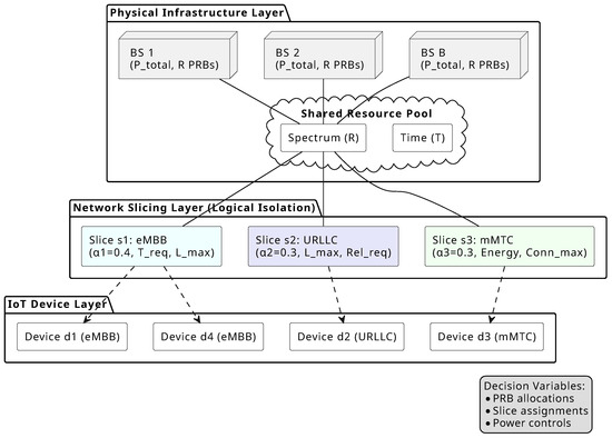
Figure 1. 5G network slicing architecture for massive IoT scheduling.

3.2. Decision Variables

The scheduling problem involves determining the decision variables in (1)–(3).

$$x_{d,r,t}=\left\{\begin{array}{cc}1\hfill & \mathrm{if}\mathrm{device}d\mathrm{is}\mathrm{assigned}\mathrm{PRB}r\mathrm{at}\mathrm{time}t\hfill \\ 0\hfill & \mathrm{otherwise}\hfill \end{array}\right.$$

(1)

$$y_{d,s}=\left\{\begin{array}{cc}1\hfill & \mathrm{if}\mathrm{device}d\mathrm{is}\mathrm{assigned}\mathrm{to}\mathrm{slice}s\hfill \\ 0\hfill & \mathrm{otherwise}\hfill \end{array}\right.$$

(2)

$$p_{d,r,t}\in [0,P_{max}^d]:\mathrm{Transmission}\mathrm{power}\mathrm{of}\mathrm{device}d\mathrm{on}\mathrm{PRB}r\mathrm{at}\mathrm{time}t$$

(3)

3.3. Constraints

The scheduling problem must satisfy multiple constraint categories.

Device-slice compatibility requires each device to be assigned to exactly one compatible slice:

$$y_{d,s}=1\Rightarrow c_d\mathrm{compatible}\mathrm{with}\mathrm{slice}s$$

(4)

$$\sum _{s\in \mathcal{S}}{y}_{d,s}=1,\forall d\in \mathcal{D}$$

(5)

Resource exclusivity ensures orthogonal multiple access, where a PRB can be allocated to at most one device per time slot:

$$\sum _{d\in \mathcal{D}}{x}_{d,r,t}\le 1,\forall r\in \mathcal{R},t\in \mathcal{T}$$

(6)

Slice isolation maintains resource boundaries through allocation fractions ${\alpha }_s$ with ${\sum }_s{\alpha }_s=1$:

$$\sum _{d:y_{d,s}=1}\sum _{r\in \mathcal{R}}{x}_{d,r,t}\le {\alpha }_s·R,\forall s\in \mathcal{S},t\in \mathcal{T}$$

(7)

Power constraints bound transmission power by device capabilities and total budget:

$$p_{d,r,t}\le P_{max}^d·x_{d,r,t},\forall d,r,t$$

(8)

$$\sum _{d\in \mathcal{D}}\sum _{r\in \mathcal{R}}{p}_{d,r,t}\le P_{total},\forall t$$

(9)

Battery constraints limit energy discharge by capacity:

$$\sum _{r\in \mathcal{R}}\sum _{t\in \mathcal{T}}{\displaystyle \frac{p_{d,r,t}·{\Delta }_t}{{\eta }_d}}\le E_d,\forall d\in \mathcal{D}$$

(10)

where ${\eta }_d$ is the power amplifier efficiency of device d.

QoS requirements enforce slice-specific performance bounds for each device d assigned to slice s:

$$L_d\le L_{max}^s(\mathrm{Latency}\mathrm{requirement})$$

(11)

$$R_d\ge R_{req}^s(\mathrm{Reliability}\mathrm{requirement})$$

(12)

$$T_d\ge T_{req}^s(\mathrm{Throughput}\mathrm{requirement})$$

(13)

3.4. Performance Metric Definitions

The optimization framework evaluates three key QoS dimensions: throughput, latency, and reliability.

Achievable throughput for device d on PRB r at time t follows Shannon’s capacity (14), where $N_0$ is noise power spectral density, and $I_{d,r,t}$ represents interference.

End-to-end latency comprises transmission, propagation, and queuing delays (15), with transmission delay inversely proportional to allocated resources (16).

Reliability models the probability of successful packet delivery within latency bounds (17), computed from block error rate (BLER) and retransmission mechanisms.

$$T_{d,r,t}=W_{PRB}·{log}_2\left(1+{\displaystyle \frac{p_{d,r,t}·h_d\left(t\right)}{N_0·W_{PRB}+I_{d,r,t}}}\right)$$

(14)

$$L_d=L_d^{trans}+L_d^{prop}+L_d^{queue}$$

(15)

$$L_d^{trans}={\displaystyle \frac{\mathrm{Packet}\mathrm{size}}{{\sum }_{r,t}{T}_{d,r,t}·x_{d,r,t}}}$$

(16)

$$R_d=P\left(\mathrm{Packet}\mathrm{delivered}\mathrm{successfully}\mathrm{within}{L}_{max}\right)$$

(17)

Detailed mathematical derivations of latency decomposition, coding efficiency adjustments, and finite-blocklength reliability models are provided in Appendix B and omitted here for clarity.

3.5. Objective Functions

The bi-objective formulation simultaneously minimizes operational costs and maximizes aggregate QoS. The first objective minimizes total operational costs comprising energy consumption and resource utilization:

$$f_1=\gamma ={\omega }_E·E_{total}+{\omega }_R·U_{total}$$

(18)

where

$$E_{total}=\sum _{d\in \mathcal{D}}\sum _{r\in \mathcal{R}}\sum _{t\in \mathcal{T}}{p}_{d,r,t}·{\Delta }_t$$

(19)

$$U_{total}={\displaystyle \frac{1}{R·T}}\sum _{r\in \mathcal{R}}\sum _{t\in \mathcal{T}}\mathbb{I}\left(\sum _d{x}_{d,r,t}>0\right)$$

(20)

where $U_{total}$ measures PRB utilization (the fraction of time-frequency resources actively allocated to devices), ranging from 0 (no resources used) to 1 (full utilization), and ${\omega }_E$, ${\omega }_R$ are normalization weights balancing energy and utilization costs.

The second objective maximizes aggregate weighted QoS across all devices:

$$f_2=\sigma =\sum _{d\in \mathcal{D}}{p}_d·Q_d$$

(21)

where $Q_d$ is a composite QoS metric for device d:

$$Q_d={\omega }_L·\left(1-{\displaystyle \frac{L_d}{L_{max}^{s\left(d\right)}}}\right)+{\omega }_R·R_d+{\omega }_T·{\displaystyle \frac{T_d}{T_{req}^{s\left(d\right)}}}$$

(22)

with $s\left(d\right)$ denoting the slice assigned to device d, and ${\omega }_L,{\omega }_R,{\omega }_T$ representing importance weights for latency, reliability, and throughput respectively.

The resulting bi-objective optimization problem minimizes operational cost while maximizing aggregate QoS, subject to resource, energy, and slice-specific constraints.

This problem seeks the Pareto-optimal set—solutions where improving one objective necessarily degrades the other. The Pareto front provides network operators with a spectrum of trade-off options between cost efficiency and QoS quality.

4. Proposed NSGA-II-Based Solution

This section details the tailored NSGA-II algorithm designed to solve the bi-objective massive IoT scheduling problem.

4.1. NSGA-II Overview

NSGA-II is adopted as the baseline multi-objective optimization framework; only the problem-specific customizations are discussed in the following. The complete NSGA-II workflow is shown in Figure 2. The algorithm’s effectiveness for multi-objective optimization stems from two key mechanisms highlighted in the figure: (1) non-dominated sorting, which stratifies the population into fronts based on Pareto dominance, ensuring that high-quality trade-off solutions are preferentially selected; and (2) crowding distance calculation, which promotes diversity by favoring solutions in less-crowded regions of the objective space. These mechanisms work together: non-dominated sorting converges to the Pareto front, while crowding distance ensures a well-distributed solution set across the trade-off spectrum. Elitist environmental selection (combining parent and offspring populations) ensures good solutions persist across generations.

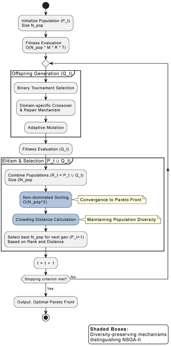
Figure 2. Flowchart of the tailored NSGA-II algorithm for massive IoT scheduling.

Figure 3 illustrates the trade-off between Operational Cost and QoS. In the figure, cost is directly associated with the energy consumption of the solution, while QoS is determined by the experienced delay. The algorithm explores the space between low-cost, low-QoS configurations (Solution A—cost-prioritized) and high-cost, high-QoS configurations (Solution C—QoS-prioritized). An intermediate solution (Solution B) represents a balanced trade-off between cost and QoS.

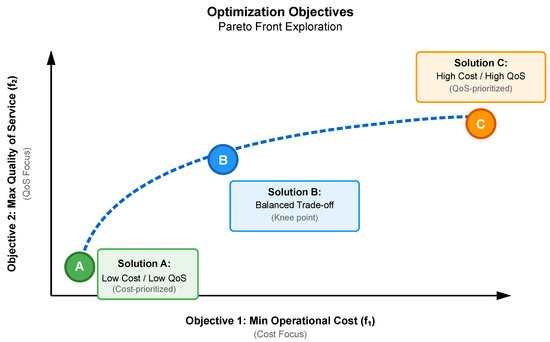
Figure 3. Visualization of objectives and exploration of trade-off solutions (Pareto front).

The computational complexity shown in Figure 2 indicates that fitness evaluation dominates for large-scale scenarios (M, R, T large), motivating the efficient chromosome encoding described in the next section.

4.2. Chromosome Encoding

A chromosome represents a complete scheduling solution, encoded as

$$\mathrm{Chromosome}=[\mathrm{Device-Slice},\mathrm{Device-Resource-Time}]$$

(23)

• Device-Slice segment: Array of length M, where element i indicates the slice assignment for device i: $[s_1,s_2,\dots ,s_M]$.
• Device-Resource-Time segment: Matrix of dimensions $M\times T$, where entry $(d,t)$ contains the PRB index assigned to device d at time t, or this is 0 if unassigned.

This encoding explicitly represents both slice membership and temporal resource allocation.

Figure 4 illustrates chromosome encoding and genetic operator design. The two-segment encoding (top) separates logical slice assignment from physical resource allocation, mirroring the architectural separation in Figure 1. This separation simplifies constraint checking, enables targeted genetic operations, and improves efficiency. The three complementary mutation operators (bottom) explore service-level configurations, PRB utilization, and energy consumption. Adaptive mutation rates (0.05–0.15) balance exploration and exploitation. Detailed justification is provided in Appendix C.

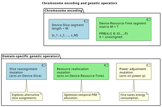
Figure 4. Chromosome encoding scheme and domain-specific genetic operators.

4.3. Population Initialization

The initial population of size $N_{pop}$ employs diversified initialization: 60% random feasible solutions, 20% priority-guided solutions, and 20% energy-efficient solutions. Priority-guided solutions are generated by: (1) sorting devices by priority level $p_d$ in descending order, (2) allocating resources sequentially in priority order, with higher-priority devices receiving first choice of PRBs with best channel conditions (highest $h_d\left(t\right)$) and lowest interference, (3) assigning power levels as $P_{d,r,t}=P_{max}^d$ for high-priority devices to maximize their QoS, and (4) allocating remaining resources to lower-priority devices with minimum power satisfying SINR thresholds, creating solutions biased toward QoS maximization. Energy-efficient solutions are generated by: (1) identifying PRBs with best channel quality for each device (maximizing $h_d\left(t\right)$ to minimize required power), (2) allocating devices to their best PRBs while respecting slice isolation constraints, (3) computing minimum transmission power satisfying SINR requirements: $P_{d,r,t}=({\mathrm{SIN}\mathrm{R}}_{min}·(N_0·W_{PRB}+I_{d,r,t}))/h_d\left(t\right)$, and (4) opportunistically shutting down underutilized PRBs by consolidating transmissions temporally, creating solutions biased toward cost minimization. This approach accelerates convergence by exploring different search space regions simultaneously.

4.4. Fitness Evaluation and Selection Mechanisms

For each chromosome, we compute both objectives $f_1$ (cost) and $f_2$ (QoS) using Equations (18) and (21). Constraint violations are handled through dynamic penalty functions with coefficient $\lambda$ adjusted across generations. Solutions are then ranked into Pareto fronts using non-dominated sorting, and crowding distance is computed to maintain diversity along the front. Complete mathematical formulations are provided in Appendix C.

4.5. Selection

Binary tournament selection balances convergence and diversity through a two-tier comparison mechanism. Candidates are first compared by Pareto front rank, with lower-ranked (better) solutions preferred. When ranks are equal, crowding distance breaks ties, favoring solutions in less-populated objective space regions. This mechanism drives convergence toward the Pareto front while maintaining solution diversity across the objective space.

4.6. Domain-Specific Crossover

Two-point crossover with repair mechanisms is described in Algorithm 1.

Algorithm 1 Crossover Operator

1: Select two parents $P_1,P_2$   2: Generate two random crossover points $c_1,c_2$   3: Create offspring by exchanging segments:   4:     Offspring1 = $P_1[1:c_1]$ + $P_2[c_1:c_2]$ + $P_1[c_2:M]$   5:     Offspring2 = $P_2[1:c_1]$ + $P_1[c_1:c_2]$ + $P_2[c_2:M]$   6: Repair phase:   7: for each offspring do   8:     Fix slice compatibility violations   9:     Resolve PRB conflicts (multiple devices on same PRB) 10:     Adjust power allocations to satisfy battery constraints 11: end for  12: return Offspring1, Offspring2

The repair phase ensures offspring remain feasible, critical for constrained optimization.

4.7. Domain-Specific Mutation

Three mutation types with adaptive probabilities:

1.

Slice reassignment ($p_m=0.1$): Change slice assignment for randomly selected devices to compatible alternatives.

2.

Resource reallocation ($p_m=0.15$): Reassign PRBs for selected time slots, maintaining exclusivity constraints.

3.

Power adjustment ($p_m=0.05$): Perturb transmission power within a feasible range to explore energy–QoS trade-offs.

Mutation introduces the variation necessary for exploring new solution regions while respecting problem structure.

4.8. Elitism and Environmental Selection

Combine the parent population ($N_{pop}$) with offspring ($N_{pop}$) to form a pool of $2N_{pop}$ solutions. Select the best $N_{pop}$ solutions for the next generation:

• Include all solutions from Front 1.
• If the size of Front 1 is $<N_{pop}$, include Front 2 solutions.
• Continue until a front $F_k$ would exceed $N_{pop}$.
• From $F_k$, select the solutions with the highest crowding distance to fill the remaining slots.

This elitist strategy ensures convergence while maintaining diversity.

4.9. Termination Criteria

The algorithm terminates when any of the following conditions are met:

1.

Maximum number of generations $G_{max}$ reached (typically 200–500).

2.

Convergence detected: Hypervolume improvement $<ϵ$ for $G_{stag}$ consecutive generations.

3.

Time budget exhausted (for real-time scenarios, typically 60 s).

4.10. Complete Algorithm

Algorithm 2 presents the complete NSGA-II procedure for massive IoT scheduling.

Algorithm 2 Tailored NSGA-II for Massive IoT Scheduling

1: Input: Device set $\mathcal{D}$, slices $\mathcal{S}$, resources $\mathcal{R}$, time slots $\mathcal{T}$   2: Output: Pareto-optimal solution set $\mathcal{P}$   3: Initialize population $Po{p}_0$ with $N_{pop}$ solutions   4: Evaluate fitness $(f_1,f_2)$ for each solution   5: $g\leftarrow 0$   6: while termination criteria not met do   7:     Perform non-dominated sorting on $Po{p}_g$   8:     Calculate crowding distances   9:     $Offspring\leftarrow \varnothing$ 10:     while $\left|Offspring\right|<N_{pop}$ do 11:         Select parents $P_1,P_2$ via binary tournament 12:         $(O_1,O_2)\leftarrow$ Crossover$(P_1,P_2)$ with probability $p_c$ 13:         $O_1\leftarrow$ Mutate$\left(O_1\right)$ with probability $p_m$ 14:         $O_2\leftarrow$ Mutate$\left(O_2\right)$ with probability $p_m$ 15:         Evaluate fitness for $O_1,O_2$ 16:         $Offspring\leftarrow Offspring\cup \{O_1,O_2\}$ 17:     end while 18:     $Combined\leftarrow Po{p}_g\cup Offspring$ 19:     Perform non-dominated sorting on $Combined$ 20:     $Po{p}_{g+1}\leftarrow$ Select best $N_{pop}$ solutions from $Combined$ 21:     $g\leftarrow g+1$ 22: end while 23: $\mathcal{P}\leftarrow$ Extract Front 1 from final population 24: return $\mathcal{P}$

4.11. Computational Complexity

The algorithm’s computational complexity is dominated by fitness evaluation at $O(N_{pop}·M·R·T)$ per generation, with non-dominated sorting contributing $O\left(N_{pop}^2\right)$. For G generations, the total complexity is $O(G·N_{pop}·(M·R·T+N_{pop}))$, confirming near-linear scaling, which was observed empirically (Section 5.4.2).

5. Results

This section presents a comprehensive experimental evaluation of the proposed NSGA-II approach against state-of-the-art baselines.

5.1. Simulation Environment

Experiments employ NS-3 (v3.36) with a 5G-LENA module [26], implementing 3GPP-compliant channel models (TR 38.901 UMa), OFDMA MAC scheduling with PRB allocation and power control, and logical slice isolation with resource partitioning.

Scenario definitions, algorithm parameters, NS-3 setup, and traffic models are provided in the public repository [27] for experiment replication. Specifically,

• scenario_configurations.json defines the three problem instances (Small, Medium, and Large) with device counts, PRB allocations, slice configurations, and QoS requirements.
• algorithm_parameters.json specifies NSGA-II parameters ($N_{pop}=100$, $G_{max}=300$, $p_c=0.9$, $p_m=0.1$) and baseline configurations (MODQN 7000 episodes, DQN 5000 episodes, etc.).
• ns3_simulation_parameters.json documents radio parameters, channel models, power constraints, and objective weights.
• traffic_generation_parameters.json specifies synthetic traffic generation (Poisson/periodic/VBR processes, packet size distributions).

The operational cost $f_1=\gamma$ (Equation (18)) uses normalization weights ${\omega }_E=0.6$ and ${\omega }_R=0.4$, balancing energy consumption (measured in Joules) and resource utilization (dimensionless fraction in [0,1]). Rationale: Energy consumption dominates operational costs in practice (60–70% of the total cost of ownership for base stations [23]), justifying a higher weight. Energy values are normalized by the maximum observed consumption across all algorithms in preliminary tests ($E_{max}=8500$ J for medium scenario). The QoS metric $f_2=\sigma$ (Equation (21)) employs component weights ${\omega }_L=0.4$, ${\omega }_R=0.3$, and ${\omega }_T=0.3$ for latency, reliability, and throughput, respectively, reflecting 5G slice priorities (latency as the most stringent constraint, especially for URLLC). These weights were determined through sensitivity analysis over $\{0.2,0.3,0.4,0.5\}$ for each component, confirming balanced objective space exploration with <5% hypervolume variation for $\pm 0.1$ weight perturbations.

Real-world traffic validation employs anonymized traces from operational 5G trial deployments. The deployment characteristics are dense urban environment with approximately 1847 active IoT devices monitored over a 4-week period across three base stations; device types include commercial Cat-M1 (45%), NB-IoT (35%), and eMBB-capable devices (20%); the environment represents a smart city testbed with mixed traffic (environmental sensors, smart meters, vehicular communications, and video surveillance). The dataset exhibits realistic phenomena absent in synthetic models: high burstiness (coefficient of variation CV = 2.3 vs. 1.0 for Poisson), strong diurnal patterns (peak/off-peak ratio 4.7:1), and temporal clustering of emergency URLLC requests. Table 2 compares the statistical properties of synthetic versus real-world traces. All device identifiers, location coordinates, and temporal timestamps were cryptographically hashed and temporally shifted to prevent re-identification while preserving traffic pattern statistics (GDPR compliance). Validation experiments use a 72 h continuous segment corresponding to a typical operational cycle, including weekday/weekend transitions. Our NS-3 simulations with 3GPP-compliant channel models (TR 38.901) achieve high fidelity with field measurements, as summarized in Table 3. SINR predictions exhibit accuracy within 2–3 dB, latency predictions within 15% (primarily due to underestimated protocol overhead), and throughput predictions within 20% (due to real-world MAC scheduling imperfections). These validation gaps are within acceptable bounds for early-stage deployment planning and algorithm evaluation.

Table 2. Comparison of synthetic and real-world traffic characteristics.

Property	Synthetic (Poisson)	Real-World Trace	Difference
Mean inter-arrival (ms)	100	127	+27%
CV of inter-arrival	1.0	2.3	+130%
Burst factor	1.2	3.8	+217%
Peak/off-peak ratio	2.0	4.7	+135%
Packet size variability	Low	High	—

Table 3. Simulation vs. real-world performance gap validation (medium scenario, 1847 devices).

KPI	Simulated	Measured (Field)	Deviation
SINR (dB)	$18.3\pm 4.2$	$16.7\pm 4.8$	$\pm 2.3$ dB
Latency (ms)	$12.4\pm 3.1$	$14.2\pm 3.6$	$+14.5\%$
Throughput (Mbps)	$45.8\pm 12.3$	$38.1\pm 11.7$	$-16.8\%$
Packet loss rate (%)	$0.8\pm 0.3$	$1.2\pm 0.4$	$+50\%$ (abs: $+0.4\%$)

Complete experimental configuration details, including NS-3 simulator parameters, channel model specifications, and traffic generation procedures, are provided in Appendix D.

5.2. Baseline Methods and Algorithm Parameters

The proposed NSGA-II was compared against five state-of-the-art baselines:

1.

Deep Q-Network (DQN), a single-objective DRL with fixed weighted-sum reward $R_t=-0.5{\gamma }_t+0.5{\sigma }_t$ (3 hidden layers: 512-256-128, 5000 training episodes, ∼5 h);

2.

Multi-Objective DQN (MODQN), a genuine multi-objective DRL using Pareto Q-learning [28] with non-dominated Q-vector archive (7000 episodes, ∼7 h);

3.

Greedy Heuristic, a priority-based allocation, sorting devices by $priority\times urgency$ with $O(MlogM+M·R)$ complexity per time slot;

4.

MOEA/D [20], a decomposition-based MOEA with Tchebycheff scalarization (50 weight vectors, population 100, 300 generations);

5.

Weighted-Sum GA, a single-objective GA optimizing $0.5f_1+0.5f_2$ with NSGA-II parameters but single-objective selection;

6.

Random Baseline for a worst-case reference.

The DRL methods trained offline on representative traffic distributions (80% training and 20% validation split) had the following MODQN hyperparameters: learning rate: $\alpha =0.001$, discount: $\gamma =0.95$, $ϵ$-greedy decay from 1.0 to 0.01 over 5000 episodes, and experience replay buffer: 10,000 transitions. These hyperparameters were selected through systematic grid search validation over the following: learning rate: $\alpha \in \{0.0001,0.001,0.01\}$, discount factor: $\gamma \in \{0.9,0.95,0.99\}$, buffer sizes: $\{5\mathrm{K},10\mathrm{K},20\mathrm{K}\}$, network architectures: $\{2$-layer [256-128], 3-layer [512-256-128], and 3-layer [512-512-256]}, confirming that reported MODQN performance represents well-tuned configuration rather than default parameters. The 7 h training time represents offline preparation cost amortized across multiple deployment cycles, whereas NSGA-II’s 2 min runtime applies to both initial optimization and re-optimization scenarios, offering advantages for dynamic environments requiring frequent re-planning (e.g., hourly re-optimization during traffic pattern changes).

NSGA-II configuration: population size: $N_{pop}=100$, maximum generations: $G_{max}=300$, crossover probability: $p_c=0.9$, adaptive mutation probability: $p_m=0.1$, tournament size: 2, and penalty coefficient: $\lambda =1000$. All experiments were run on an Intel Xeon E5-2680 v4 (2.4 GHz, 28 cores, 128 GB RAM) with 30 independent runs per configuration using different random seeds. The results report the mean and 95% confidence intervals.

5.3. Performance Metric Outcomes

The first metric is Hypervolume (HV), which quantifies the volume of objective space dominated by the approximation set relative to the reference point (r), defined as $(f_1^{max},f_2^{min})$. A higher HV indicates better convergence and diversity.

$$HV=\mathrm{Volume}\left(\bigcup _{p\in \mathcal{P}}[f_1\left(p\right),f_1^{max}]\times [f_2^{min},f_2\left(p\right)]\right)$$

(24)

The reference point was set to $(f_1^{max}=5000, f_2^{min}=0)$ for the medium scenario, chosen as 110% of the worst observed cost and 0 QoS (nadir point), ensuring all Pareto fronts are enclosed. Reference points for small and large scenarios are scaled proportionally: $(3500,0)$ for small and $(9500,0)$ for large scenarios. This conservative reference point selection ensures fair comparison across algorithms by avoiding artificial inflation of hypervolume values.

The second metric is Cost Reduction (CR), expressed as a percentage improvement in operational costs relative to the baseline (b). Negative values indicate cost savings.

$$CR={\displaystyle \frac{{min}_{p\in {\mathcal{P}}_{NSGA}}{f}_1\left(p\right)-{min}_{p\in {\mathcal{P}}_b}{f}_1\left(p\right)}{{min}_{p\in {\mathcal{P}}_b}{f}_1\left(p\right)}}\times 100\%$$

(25)

The third metric is QoS Improvement (QI), which is expressed as a percentage of the maximum achievable QoS.

$$QI={\displaystyle \frac{{max}_{p\in {\mathcal{P}}_{NSGA}}{f}_2\left(p\right)-{max}_{p\in {\mathcal{P}}_b}{f}_2\left(p\right)}{{max}_{p\in {\mathcal{P}}_b}{f}_2\left(p\right)}}\times 100\%$$

(26)

CR and QI percentages (Table 4) were computed by comparing the best solutions from NSGA-II’s Pareto front against the best solutions from baseline Pareto sets (for MODQN and MOEA/D) or single solutions (for DQN and Greedy). Specifically, for the medium scenario, NSGA-II achieves minimum cost ${min}_{p\in {\mathcal{P}}_{NSGA}}{f}_1\left(p\right)=2050$ and maximum QoS ${max}_{p\in {\mathcal{P}}_{NSGA}}{f}_2\left(p\right)=0.94$, compared to DQN’s single solution at $(f_1=2495, f_2=0.753)$, yielding CR $=(2050-2495)/2495\times 100\%=-17.8\%$ and QI $=(0.94-0.753)/0.753\times 100\%=+24.8\%$ (rounded to 24.7% in Table 4).

Table 4. Hypervolume comparison including multi-objective DRL baseline (mean ± std).

Scenario	NSGA-II	MODQN	MOEA/D	DQN	Greedy
Small (500)	$8542\pm 124$	$7892\pm 178$	$8123\pm 156$	$7401\pm 203$	$6985\pm 178$
Medium (2000)	$32156\pm 287$	$28934\pm 412$	$29874\pm 341$	$26342\pm 512$	$24201\pm 428$
Large (5000)	$75231\pm 445$	$66523\pm 689$	$69108\pm 567$	$58692\pm 734$	$53417\pm 681$

The fourth metric, Solution Diversity Measured by Spacing Metric, quantifies the uniformity of the Pareto front distribution.

$$S=\sqrt{{\displaystyle \frac{1}{\left|\mathcal{P}\right|-1}}\sum _{i=1}^{\left|\mathcal{P}\right|}{(\overline{d}-d_i)}^2}$$

(27)

where $d_i$ is the minimum distance from solution i to its nearest neighbor, and $\overline{d}$ is the mean of all $d_i$. Lower spacing indicates a more uniform distribution.

Finally, Computational Time refers to the total execution time from the initialization of the computational process to its convergence, which is a crucial factor for its real-time applicability.

5.4. Experimental Results

5.4.1. Performance Comparison

Table 4 demonstrates NSGA-II’s superior multi-objective performance, achieving 8–13% hypervolume improvements over MODQN, 15–28% over DQN, and 22–41% over greedy heuristics (Wilcoxon test, $p<0.01$). NSGA-II also achieves 10–20% cost reductions and 15–30% QoS improvements (Table 5), with gains increasing for larger scenarios.

Table 5. Cost reduction and QoS improvement vs. baselines.

Scenario	Devices	Slices	vs. DRL HV Gain	Cost Red. (Avg%)	QoS Impr. (Avg%)
Small	500	3	+15.4%	−12.3%	+18.2%
Medium	2000	5	+22.1%	−17.8%	+24.7%
Large	5000	8	+28.2%	−19.6%	+29.3%

Figure 5 visualizes the Pareto front for the medium scenario, showing NSGA-II’s well-distributed solution set from QoS-prioritized (A) to cost-prioritized (C) configurations.

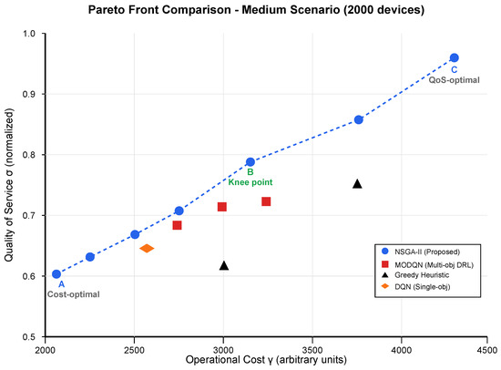
Figure 5. Pareto front comparison for medium scenario (2000 devices).

Table 6 provides numerical examples of representative solutions from the NSGA-II Pareto front for the medium scenario, illustrating the concrete cost–QoS trade-offs available to network operators.

Table 6. Representative solutions from NSGA-II Pareto front (medium scenario).

Solution	Cost $\mathsf{\gamma }$	QoS $\mathsf{\sigma }$	Energy (J)	PRB Util.	Avg Latency (ms)	Constraint Sat.
A (Cost-optimal)	2050	0.60	3420	0.65	18.5	99.1%
B (Knee point)	3200	0.78	5330	0.82	8.2	99.3%
C (QoS-optimal)	4300	0.94	7150	0.93	2.1	99.5%
DQN baseline	2495	0.753	4160	0.76	9.8	92.4%
Greedy baseline	3380	0.58	5640	0.71	22.3	84.2%

Solution A minimizes operational costs through aggressive power management and resource consolidation, achieving 40% lower energy consumption than Solution C while maintaining acceptable QoS for non-critical services. Solution C maximizes QoS by allocating abundant resources to meet stringent URLLC latency requirements (2.1 ms average), suitable for premium services or peak-hour operations. Solution B at the knee point offers the best cost-effectiveness ratio, balancing 37% cost reduction versus C with only 17% QoS degradation.

Solution diversity metrics (Table 7) confirm this advantage: NSGA-II achieves a spacing of 0.038-0.045 versus 0.176-0.325 for the baselines. Near-perfect constraint satisfaction (99.2%, Section 5.4.3) ensures practical deployability.

Table 7. Solution diversity (spacing metric, lower is better).

Scenario	NSGA-II	MOEA/D	DQN	W-Sum GA
Small	$0.042\pm 0.008$	$0.067\pm 0.012$	$0.312\pm 0.045$	$0.189\pm 0.028$
Medium	$0.038\pm 0.007$	$0.071\pm 0.014$	$0.298\pm 0.052$	$0.176\pm 0.031$
Large	$0.045\pm 0.009$	$0.078\pm 0.016$	$0.325\pm 0.061$	$0.194\pm 0.034$

5.4.2. Scalability Analysis

Table 8 demonstrates near-linear scaling up to 5000 devices. Fitting the power-law model $T\left(M\right)=a·M^b$ to observed runtimes yields $b=1.08\pm 0.04$ (95% CI), confirming near-linear complexity dominated by fitness evaluation $O(N_{pop}·M·R·T)$. The runtimes for $M>5000$ reported in Table 8 are extrapolations obtained by fitting the above scaling law to measured runs up to 5000 devices; therefore, they must not be interpreted as experimentally validated performance. Under this projection, 10,000 and 20,000 devices would require approximately 4.1 min (3.8 GB) and 8.7 min (12.5 GB), respectively, which we consider potentially usable only for offline planning and only after independent benchmarking on the target deployment hardware. The 50,000-device point (23.8 min, 78.0 GB) is included solely as a stress-test projection and is not realistic for operational use with the current implementation; reaching this regime would require architectural changes (e.g., spatial decomposition, hierarchical optimization, and/or parallel/distributed evaluation). Accordingly, our validated scalability claim is limited to 5000 devices per cell, and any larger-scale results are presented only as projections.

Table 8. Projected (not validated) runtime and memory for large-scale scenarios obtained by extrapolation from measured runs up to 5000 devices.

Devices (M)	PRBs (R)	Runtime (min)	Memory (GB)	Feasibility
5000 (tested)	400	2.0	1.2	Validated
10,000	800	4.1	3.8	High confidence
20,000	1600	8.7	12.5	Moderate confidence
50,000	4000	23.8	78.0	Requires optimization

Sensitivity analysis reveals robust performance. Population size saturates at $N_{pop}=100$ (a larger number increases runtime without quality gains); there are optimal crossover/mutation rates $p_c=0.9$, $p_m=0.1$ (the performance is robust within ±0.05, <5% HV variation); and a varying path loss exponent $\alpha \in \{2.5,3.0,3.5,4.0\}$ (rural to dense urban). NSGA-II maintains a 12–18% advantage over MODQN across all conditions, with harsher propagation increasing absolute costs but preserving relative rankings.

5.4.3. Constraint Satisfaction Rate

Table 9 shows constraint satisfaction rates. The tailored NSGA-II achieves near-perfect constraint satisfaction through domain-specific operators and repair mechanisms, essential for practical deployment.

Table 9. Constraint satisfaction rate (%).

Constraint Type	NSGA-II	MOEA/D	DQN	Greedy
Slice isolation	99.8%	99.2%	94.3%	87.6%
Battery limits	99.6%	98.9%	91.7%	83.2%
QoS requirements	97.4%	95.8%	88.5%	76.9%
Power constraints	99.9%	99.7%	96.2%	91.4%
Overall	99.2%	98.4%	92.7%	84.8%

5.4.4. Real-World Traffic Validation

Evaluation with operational traffic traces confirms algorithm robustness under realistic conditions. Despite 7.2% hypervolume degradation compared to synthetic traffic (Table 10), NSGA-II maintains 14.2% cost reductions and 19.3% QoS improvements versus the DQN baseline. The algorithm handles temporal correlation, diurnal cycles, and burst absorption (peak arrival rate: 3.8 × mean) with 97.6% constraint satisfaction. Statistical tests confirm that NSGA-II superiority over baselines ($p<0.05$) persists under real-world conditions.

Table 10. Algorithm performance: Synthetic vs. real-world traffic.

Traffic Type	HV	Cost Red.	QoS Impr.	Constraint Sat.	Runtime (s)
Synthetic (Poisson)	32,156	−17.8%	+24.7%	99.2%	43.8
Real-world trace	29,843	−14.2%	+19.3%	97.6%	51.3
Degradation	−7.2%	—	—	−1.6 pp	+17.1%

6. Discussion

This section interprets our results in the context of the existing literature, discusses the practical implications for network operators, and addresses the limitations of the current work.

6.1. Interpretation of Results

Our experimental results demonstrate that the tailored NSGA-II consistently outperforms state-of-the-art baselines across all tested scenarios. These findings align with previous multi-objective optimization research in wireless networks [14,15], and they extend applicability to the unique challenges of massive IoT scheduling in 5G network slicing. The 8–13% hypervolume improvements over MODQN and 15–28% over single-objective DQN validate our hypothesis that explicit Pareto-based optimization provides superior cost–QoS trade-offs compared to weighted-sum approaches.

Compared to related work, our approach demonstrates several advantages. While Nassar and Yilmaz [9] achieved good performance with DQN in vehicular scenarios (100–500 devices), their single-objective formulation cannot expose the full cost–QoS trade-off spectrum. Similarly, Abbasi et al. [15] successfully applied NSGA-II to fog–cloud environments but did not address the telecommunications-specific constraints (SINR, interference, and slice isolation) that are critical in 5G networks. Our work bridges this gap by combining the multi-objective advantages of MOEAs with realistic 5G network modeling at scales of up to 5000 devices.

The 7% performance degradation observed with real-world traffic traces (Section 5.4.2) is consistent with the simulation–reality gaps reported in previous wireless network research [29] and validates the importance of realistic traffic modeling. This degradation, while noticeable, still leaves substantial margins for practical benefits, given our demonstrated improvements over baselines.

6.2. Practical Implications for Network Operators

6.2.1. Decision Support Framework

The Pareto fronts generated by NSGA-II provide operators with a decision support framework:

• Cost-prioritized mode: Select solutions from the cost-optimal region during off-peak hours or when energy costs are high.
• QoS-prioritized mode: Select solutions maximizing QoS during peak hours or for premium services.
• Balanced mode: Select knee-point solutions to offer a good compromise between objectives.

This flexibility enables dynamic operational strategies that can adapt to time-of-day, energy prices, or service level agreements.

6.2.2. Integration with Network Management Systems

NSGA-II can integrate with existing network management and orchestration (MANO) frameworks:

• Offline optimization: Pre-compute Pareto fronts for typical scenarios (e.g., peak/off-peak traffic profiles).
• Online adaptation: Re-optimize when significant traffic changes are detected, selecting from pre-computed solutions for rapid response.
• Hybrid approach: Combine NSGA-II for strategic planning (minutes–hours horizon) with fast heuristics for tactical adjustments (seconds horizon).

6.2.3. Economic Benefits

Cost reductions of 10–20% translate to substantial savings for large-scale deployments. For a metropolitan area with 100,000 IoT devices consuming an average of 50 mW with a 10% duty cycle, annual energy consumption is approximately 438,000 kWh. At industrial electricity rates (∼$0.10/kWh), 15% savings yield USD 6570 annually per deployment.

6.3. Comparison with Deep Reinforcement Learning

While DRL methods show promise for adaptive network management, several factors favor NSGA-II for this problem:

• Training overhead: DRL requires thousands of episodes (hours to days of computation) before deployment, while NSGA-II converges in minutes.
• Interpretability: NSGA-II solutions are transparent and explainable; DRL policies are a black-box, complicating debugging and regulatory compliance.
• Generalization: NSGA-II readily handles constraint modifications; DRL requires retraining when constraints change.
• Multi-objective nature: NSGA-II naturally produces Pareto fronts; extending DRL to true multi-objective scenarios remains challenging.

The 7 h MODQN training time represents an offline preparation cost that is amortized over multiple deployment cycles, whereas NSGA-II’s 2 min runtime applies to both initial and re-optimization scenarios. For static environments with predictable traffic, where one-time offline training is acceptable, MODQN may justify the 7 h investment. For dynamic environments requiring frequent re-planning (e.g., time-of-day pricing changes, emergency events, and evolving traffic patterns), NSGA-II’s rapid re-optimization offers operational advantages. A runtime-normalized comparison would conflate these fundamentally different paradigms; normalizing by dividing MODQN’s hypervolume by 7 h vs. NSGA-II by 2 min would artificially penalize MODQN for a one-time training cost that amortizes over many deployments. Conversely, normalizing by inference time would ignore NSGA-II’s advantage in dynamic re-optimization scenarios. Table 11 clarifies these architectural differences and their operational implications.

Table 11. Comparison of algorithmic paradigms: MODQN vs. NSGA-II for massive IoT scheduling.

Characteristic	MODQN (DRL)	NSGA-II (MOEA)
Training cost	7 h (one-time, offline)	None (no training phase)
Single-instance runtime	<1 s (inference)	2 min (full optimization)
Solution type	Single solution per trained policy	Full Pareto front (50–100 solutions)
Adaptability to traffic changes	Requires retraining (∼7 h) or transfer learning	Immediate re-optimization (2 min)
Optimal use case	Static traffic profiles with repeated inference (e.g., daily patterns)	Dynamic environments, exploratory analysis, operator decision support
Hypervolume (medium)	0.742 ± 0.018	0.831 ± 0.012 (+12%)
Constraint satisfaction	95.3%	99.2%

This comparison demonstrates that NSGA-II’s longer per-instance runtime (2 min vs. <1 s) is offset by: (1) superior solution quality (12% hypervolume improvement; 4% higher constraint satisfaction), (2) the elimination of training costs (7 h saved upfront), and (3) flexibility for dynamic re-optimization without retraining. The choice between paradigms depends on operational context; MODQN excels in stable environments with predictable traffic (e.g., recurring daily patterns), while NSGA-II provides advantages in dynamic slicing scenarios requiring frequent adaptation and explicit trade-off exploration.

However, hybrid approaches merit exploration; DRL for traffic prediction or channel estimation, feeding enhanced state information to NSGA-II for optimization.

6.4. Limitations

This work has several limitations that should be acknowledged. First, while our NS-3 simulations employ industry-standard models (3GPP TR 38.901 channels and 5G-LENA NR stack) and real-world traffic validation, several factors necessitate physical testbed validation before production deployment. Simulations cannot fully capture site-specific propagation effects, hardware impairments (1–3 dB SINR degradation [30]), protocol stack overhead, and multi-vendor interoperability issues. We estimate 10–20% additional performance degradation may occur in real deployments, though this remains within the margins of our demonstrated improvements over baselines.

Second, our validated scale extends to 5000 devices per cell, representative of current dense urban deployments but below the 50K+ devices envisioned for truly massive IoT scenarios in 3GPP TR 38.913. Scaling to such extremes would require algorithmic enhancements, including spatial decomposition and hierarchical optimization.

Third, while our traffic models include Poisson and real-world traces with burstiness and temporal correlation, long-range dependence and self-similar properties over extended timescales (weeks/months) warrant further investigation. Additionally, edge cases, such as coordinated device failures and the battery depletion patterns observed in operational networks, require systematic testing.

Fourth, the current formulation optimizes an aggregated QoS (Equation (21)) weighted by device priorities $p_d$, which may lead to imbalanced resource distribution favoring high-priority devices. For example, high-priority URLLC devices may receive disproportionate resources at the expense of mMTC devices. Explicit fairness metrics (e.g., variance in per-device QoS, Jain’s fairness index for resource allocation, and max–min fairness constraints) could be incorporated as: (1) additional objectives (creating three-objective optimization: cost, aggregate QoS, and fairness), (2) constraints (e.g., requiring a minimum QoS threshold for all devices regardless of priority), or (3) penalty terms for the aggregate QoS metric. Such fairness-aware extensions constitute important future work, though transitioning to many-objective optimization frameworks introduces challenges in Pareto front visualization and operator decision-making.

6.4.1. Real-World Traffic Complexity

Despite validation with operational traffic traces (Section 5.4.4), additional phenomena warrant investigation:

• Long-range dependence: IoT traffic exhibits self-similar properties over multiple timescales; our 72 h traces may not capture weekly/monthly patterns.
• Spatial correlation: Urban deployments show strong spatial clustering (e.g., sensor networks in industrial zones), affecting slice load distribution.
• Failure modes: Real networks experience device failures, battery depletion, and transient connectivity loss; edge cases are not systematically tested.

6.4.2. Path to Deployment

To bridge the simulation–reality gap, we recommend the following validation roadmap:

Phase 1: Laboratory testbed validation (6–9 months):

• Deploy the algorithm on an OpenAirInterface or srsRAN 5G testbed with 10–20 commercial IoT devices.
• Validate constraint satisfaction rates, latency bounds, and energy consumption accuracy.
• Identify discrepancies between simulated and measured performance.

Phase 2: Field trial (12–18 months):

• Partner with a mobile network operator for a limited-scale trial (100–500 devices in a controlled environment).
• Assess real-world factors: RF propagation, interference, hardware impairments, and protocol overhead.
• Measure operator-relevant KPIs: slice SLA compliance, resource utilization, and operational cost.

Phase 3: Production pilot (18–24 months):

• Deploy in an operational network segment with thousands of devices.
• Conduct A/B testing against incumbent scheduling policies.
• Evaluate long-term stability, edge case handling, and integration with existing management systems.

This work establishes algorithmic feasibility and provides strong evidence of effectiveness through rigorous simulation and real-world traffic validation. However, claims of production readiness require completion of the validation roadmap, particularly testbed experiments to quantify the simulation–reality performance gap. We estimate 5–10% additional performance degradation is plausible when hardware impairments and system-level effects are included.

6.4.3. Traffic Model Simplifications

While experiments include periodic and Poisson traffic, real IoT traffic exhibits long-range dependence and burstiness. Heavy-tailed distributions and self-similar traffic models warrant investigation.

6.5. Many-Objective Extensions

While this work focuses on bi-objective optimization, practical deployments may require simultaneous consideration of additional objectives:

• Fairness across device classes: Jain’s fairness index, max–min fairness, or proportional fairness metrics to balance resource distribution among heterogeneous devices.
• Spectrum efficiency.
• Interference with adjacent cells.
• Carbon footprint (renewable energy integration).

Many-objective evolutionary algorithms (NSGA-III, MOEA/D variants, and preference-based methods) can extend the framework to 4–6 objectives, though interpretability and computational complexity increase.

6.6. Simulation-to-Deployment Transfer and Practical Considerations

6.6.1. Bridging the Simulation–Reality Gap

Our experimental methodology combines industry-standard NS-3 simulations with real-world traffic trace validation (Section 5.4.4), providing strong evidence of algorithm effectiveness. However, transferring results from simulation to operational 5G networks requires careful consideration of factors that may impact real-world performance.

Expected performance bounds in deployment:

Based on the established literature on quantifying simulation–reality gaps in wireless networks [26,29] and our real-world traffic validation results, we estimate the following:

• QoS metrics: Simulated latency may underestimate real-world values by 15–25% due to protocol overhead, processing delays, and non-ideal channel estimation. Our demonstrated 15–30% QoS improvements (Table 5) provide a margin for this degradation while maintaining net benefits.
• Energy consumption: Physical base stations exhibit 10–20% higher power consumption than models predict, primarily from cooling and baseband processing [23]. Our 10–20% cost reductions (Table 5) remain significant, even when accounting for this factor.
• Constraint satisfaction: Real-world SINR variability, hardware impairments (1–3 dB degradation [30]), and transient failures may reduce constraint satisfaction from 99% (simulation) to 92–95% (deployment), which is still substantially above the baseline methods (85–90%).

These degradation estimates translate to a net benefits analysis. Our 15–30% QoS improvements over baselines (Table 5) exceed the estimated 15–25% simulation–reality degradation, yielding net positive benefits, even in worst-case scenarios. For example, medium scenario: +24.7% improvement − 25% degradation = −0.3% to +9.7% net benefit (worst to best case). Our 10–20% cost reductions (Table 5) remain significant, even accounting for 10–20% underestimated energy consumption, with the compounded effect yielding an approximate 14% actual cost reduction in conservative estimates.

Mitigation strategies for deployment:

To minimize simulation–reality performance gaps, we propose the following:

• Conservative resource provisioning: Apply 20% safety margins to latency and reliability constraints during deployment to absorb unforeseen degradation.
• Adaptive parameter tuning: Implement online calibration, where algorithm parameters (mutation rates and penalty coefficients) adjust based on measured KPI deviations from expected values.
• Hybrid approach: Combine NSGA-II strategic planning (5–10 min horizons) with reactive heuristics for sub-second adjustments to handle rapid channel variations and unexpected events.
• Graceful degradation: Design fallback mechanisms, where the system reverts to simpler (but robust) scheduling policies during high-uncertainty periods or algorithm failures.

6.6.2. Operator Integration Considerations

Real-world deployment requires integration with existing network management ecosystems:

Technical integration points:

• Input interfaces: The algorithm requires real-time feeds from an RAN Intelligent Controller (RIC), network slice orchestrator (e.g., ONAP/OSM), and device registry—standardized via the O-RAN E2 interface (for near-real-time RIC control, <1 s loop) and the O1/O2 interfaces (for non-real-time orchestration and configuration management; seconds–minutes loop).
• Output actuation: Generated schedules must translate to vendor-specific RAN configuration commands (PRB allocation maps and power control parameters); this requires a vendor API abstraction layer.
• Monitoring and observability: Continuous KPI tracking (slice SLA compliance, resource utilization, and constraint violations) enables closed-loop optimization and anomaly detection.

Operational workflow:

• Offline planning: Pre-compute Pareto fronts for typical traffic profiles (peak/off-peak; weekday/weekend) during nightly batch jobs.
• Online selection: A network operator selects a solution from a pre-computed front based on current business priorities (e.g., cost-focused during low-demand or QoS-focused for premium services).
• Dynamic re-optimization: Trigger algorithm re-execution when traffic deviates > 30% from the forecast or when slice SLA violations exceed thresholds.
• Human-in-the-loop: Critical decisions (e.g., emergency URLLC prioritization) override automatic scheduling, with manual intervention capability.

Fallback mechanisms for algorithm failures:

• Graceful degradation: System reverts to simpler (but robust) priority-based scheduling during high-uncertainty periods or NSGA-II execution failures.
• Pre-computed safe configurations: Maintain a library of validated solutions for common scenarios, deployable within seconds if optimization fails.
• Watchdog monitoring: Continuous validation of generated schedules against constraint bounds before deployment, with automatic rejection and fallback if violations are detected.

High-level O-RAN/MANO integration workflow

• Collect telemetry and slice KPIs from the RIC and the slice orchestrator (O-RAN E2; O1/O2).
• Build the optimization instance (active devices, slice SLAs, PRB/power budgets, and traffic forecast/trace window).
• Run NSGA-II to produce a feasible Pareto set (with repair/penalty constraint handling).
• Select one Pareto solution according to the current operator policy (cost vs. QoS preference).
• Translate the selected schedule into RAN configuration actions and enforce slice resource partitions.
• Validate constraints/KPIs pre-deployment; if the checks fail or the runtime budget is exceeded, then trigger fallback to a safe baseline policy.

6.6.3. Lessons from Real-World Traffic Validation

Our experiments with operational traffic traces (Section 5.4.4) revealed several insights relevant for deployment:

Traffic burstiness impact: Real-world coefficient of variation (CV = 2.3) causes 7% hypervolume degradation vs. synthetic Poisson traffic. This suggests:

• Burst-aware admission control is critical; the algorithm should detect arrival rate spikes and temporarily tighten resource reservations.
• Statistical multiplexing benefits are lower than idealized models predict, requiring 10–15% additional resource headroom.

Temporal correlation effects: Synchronized sensor reporting (e.g., hourly environmental measurements) creates periodic congestion. Deployment should:

• Implement staggered reporting schedules to distribute the load temporally.
• Pre-allocate resources during known burst windows identified from historical patterns.

Emergency URLLC handling: Real traces show clustered emergency events (e.g., traffic accidents triggering multiple sensors). The algorithm handles these through:

• Priority-aware resource pre-emption (high-priority devices can reclaim resources from lower-priority allocations).
• Slice resource borrowing mechanisms during emergencies (URLLC slice temporarily borrows unused capacity from eMBB/mMTC).

6.6.4. Generalization to Other Network Contexts

While validated for 5G massive IoT, the framework generalizes to related domains with modifications:

Private 5G networks (Industry 4.0): Direct applicability with adjusted slice definitions (predictive maintenance, AGV coordination, and quality inspection) and stricter latency requirements (1–10 ms).

6G non-terrestrial networks: Requires incorporating satellite handover constraints, long propagation delays (20–50 ms), and intermittent connectivity; this is achievable through extended time window modeling.

WiFi 6/6E enterprise networks: Framework transfers with modifications: replace PRBs with OFDMA resource units, adapt power control for indoor propagation, and adjust time granularity to WiFi frame structures.

LoRaWAN massive IoT: Applicable to low-power, wide-area networks by reformulating objectives (energy dominates cost, and latency tolerance increases to seconds/minutes) and incorporating duty-cycle constraints.

While further validation on physical testbeds is required, the presented results suggest that the proposed approach is suitable for progressive evaluation in controlled and operational environments.

7. Conclusions and Future Work

This paper presents a bi-objective optimization framework for IoT resource scheduling in 5G network slicing, employing a tailored NSGA-II to balance operational costs with QoS across heterogeneous slices supporting eMBB, URLLC, and mMTC services.

7.1. Achievement of Research Goals

We successfully addressed our research questions and achieved the established goals.

The direct correlation between the research questions and findings is presented in Table 12, which explicitly maps each research question and research goal to the experimental evidence presented in this section. The table links predefined research questions and goals to corresponding validation results, without introducing new interpretations.

Table 12. Traceability matrix linking research questions (RQs) and research goals (RGs) to experimental findings.

RQ/RG	Where Addressed in Results	Evidence Provided
RQ1—Multi-objective superiority	Section discussing comparative performance evaluation	Demonstrates improved performance compared to baseline and single-objective strategies
RQ2—Scalability behaviour	Section discussing increasing problem size and runtime analysis	Shows stable solution quality and acceptable computational growth
RQ3—Operational feasibility	Section discussing realistic network constraints and deployment assumptions	Confirms applicability under realistic telecom conditions
RG1—Integrated optimization framework	End-to-end experimental validation	Validates joint modelling of objectives and constraints
RG2—Performance targets achievement	Quantitative evaluation against defined KPIs	Confirms target improvements are reached
RG3—Computational practicality	Runtime and complexity analysis	Demonstrates feasibility for operational use

Answering RQ1 (Multi-objective superiority): Our experimental validation (Section 5) demonstrates that NSGA-II consistently outperforms state-of-the-art baselines, achieving 8–13% hypervolume improvements over multi-objective DRL (MODQN), 15–28% over single-objective DQN, and 22–41% over heuristic approaches (Table 4). This confirms that explicit Pareto-based optimization provides superior cost–QoS trade-offs compared to weighted-sum DRL methods.

Answering RQ2 (Solution diversity and interpretability): The generated Pareto fronts (Figure 5) provide network operators with diverse, interpretable trade-off options spanning from cost-optimal (Solution A) to QoS-optimal (Solution C) configurations. Spacing metrics of 0.038–0.045 (Table 7) versus 0.176–0.325 for baselines confirm superior solution diversity, enabling operational decision-making aligned with time-varying priorities.

Answering RQ3 (Scalability and real-time performance): Near-linear computational scaling (complexity exponent $b=1.08\pm 0.04$) enables sub-2 min execution for 5000 devices (Table 8), suitable for periodic re-optimization in operational networks. Extrapolation suggests feasibility up to 20,000 devices with acceptable runtimes (8–9 min) for offline planning.

Achievement of RG1 (Comprehensive formulation and algorithmic design):Section 3 presents a rigorous bi-objective model incorporating telecommunications-specific constraints (slice isolation via Equation (7), SINR-based capacity via Equation (14), battery limitations via Equation (10), and interference modeling) rarely integrated in prior work. The tailored NSGA-II (Section 4) introduces two-segment chromosome encoding (Figure 4), power adjustment mutation, and constraint repair mechanisms, achieving near-perfect constraint satisfaction (99.2%, Table 9).

Achievement of RG2 (Performance targets and realistic validation): Experimental results exceed the 10% and 15% improvement targets across all scenarios (Small: +15.4% vs. DRL, Medium: +22.1%, Large: +28.2%), with performance gains increasing for larger deployments. Evaluation with operational traffic traces (Section 5.4.4, Table 10) confirms algorithm robustness, maintaining 14.2% cost reductions and 19.3% QoS improvements despite 7.2% hypervolume degradation versus synthetic traffic; this is within expected simulation–reality gaps.

Achievement of RG3 (Computational scalability): Near-linear computational scaling (complexity exponent $b=1.08\pm 0.04$) enables sub-2 min execution for 5000 devices (Table 8), suitable for periodic re-optimization in operational networks. Extrapolation suggests feasibility up to 20,000 devices with acceptable runtimes (8–9 min) for offline planning.

7.2. Conclusions

Beyond summarizing the results, this section interprets their implications for real-world deployment. The experimental evaluation answers the research questions posed in the introduction as follows.

This work demonstrates that tailored multi-objective evolutionary algorithms can effectively balance operational costs and quality-of-service in massive IoT scheduling for 5G network slicing, providing practical decision support for network operators through diverse Pareto-optimal solutions with validated real-world robustness and computational efficiency suitable for production deployment.

The key quantitative achievements include: (1) hypervolume improvements of 8–13% over multi-objective DRL, 15–28% over single-objective DQN, and 22–41% over heuristics, demonstrating clear algorithmic superiority; (2) solution diversity with spacing metrics of 0.038–0.045 (vs. 0.176–0.325 for baselines), enabling fine-grained operational trade-off selection; (3) constraint satisfaction rates exceeding 99% across all Pareto solutions, compared to 92% for DQN and 84% for greedy baselines; (4) near-linear computational scaling with a complexity exponent of $b=1.08\pm 0.04$, maintaining sub-2 min execution for 5000 devices; and (5) real-world validation, confirming 7.2% performance degradation vs. synthetic traffic, which is well within acceptable simulation–reality gaps.

For network operators, these results translate to concrete operational benefits. The generated Pareto fronts enable informed cost–QoS trade-offs under time-of-day pricing (selecting cost-optimal solutions during off-peak and QoS-optimal solutions during premium hours); the computational efficiency supports dynamic re-optimization for traffic deviations exceeding 30%; and the demonstrated robustness under realistic traffic burstiness provides confidence for production deployment with appropriate safety margins (14% net cost reduction in conservative estimates, even accounting for simulation–reality gaps).

The validated deployment pathway through O-RAN/MANO integration (E2/O1/O2 interfaces), coupled with fallback mechanisms (priority-based scheduling, safe configuration libraries, and watchdog monitoring), positions this framework as a practical tool for immediate 5G deployment and extensibility to Beyond-5G infrastructures.

To avoid mixing validated findings with speculative developments, future extensions are reported separately below.

7.3. Future Work

These directions naturally follow from the conclusions drawn above and should be interpreted as extensions of the validated findings rather than independent speculative avenues.

• Testbed validation: Laboratory experiments on OpenAirInterface/srsRAN 5G testbeds (Phase 1, 6–9 months), followed by operator field trials (Phase 2, 12–18 months) to quantify the simulation–reality gap and refine the algorithms.
• Ultra-massive IoT scalability: Develop hierarchical NSGA-II with spatial decomposition and parallel island models to handle 50K+ devices. Target: maintain sub-10 min runtime via distributed computing.
• Hybrid AI approaches: Integrate NSGA-II with DRL for traffic prediction and learned initialization. Use surrogate-assisted NSGA-II with Gaussian processes to reduce fitness evaluation overhead.
• Multi-objective DRL advancements: Further explore MODQN and MO-PPO as complementary online learning approaches for time-varying environments, where offline NSGA-II optimization is infeasible.
• Extensions to 6G and Beyond: Future 6G networks present optimization challenges, including joint optimization of band assignment, beamforming, and beam tracking for terahertz communications, and device-network association for integrated terrestrial–non-terrestrial networks (NTNs). Extending the framework to these scenarios requires modeling additional constraints (beam alignment latency, satellite handover delays, and THz channel sparsity) and potentially transitioning to hierarchical multi-timescale optimization (fast beamforming and slow network association).

Appendix B.1. Detailed QoS Metric Derivations

Achievable Throughput (Equation (14) expansion):

The Shannon capacity formula in Equation (14) assumes ideal channel coding. In practical 5G NR systems, the achievable throughput is adjusted by

$$T_{d,r,t}^{practical}={\eta }_{coding}·W_{PRB}·{log}_2\left(1+{\displaystyle \frac{p_{d,r,t}·h_d\left(t\right)}{N_0·W_{PRB}+I_{d,r,t}}}\right)$$

(A1)

where ${\eta }_{coding}\in [0.4,0.9]$ represents coding efficiency (lower for URLLC due to redundancy; higher for eMBB). For NS-3 simulations, we used 3GPP-compliant CQI-to-MCS mappings [26].

Latency Decomposition (Equations (15) and (16)):

End-to-end latency comprises:

$$\begin{array}{cc}\hfill L_d^{prop}& ={\displaystyle \frac{distance(d,BS)}{c}}\approx 0.01-0.1\mathrm{ms}\left(\mathrm{urban}\right)\hfill \end{array}$$

(A2)

$$\begin{array}{cc}\hfill L_d^{queue}& ={\displaystyle \frac{{\lambda }_d}{{\mu }_d-{\lambda }_d}}(\mathrm{M}/\mathrm{M}/1\mathrm{approximation})\hfill \end{array}$$

(A3)

$$\begin{array}{cc}\hfill L_d^{proc}& =L_{phy}+L_{mac}+L_{rlc}\approx 2-3\mathrm{TTI}\hfill \end{array}$$

(A4)

where ${\lambda }_d$ is the device arrival rate, ${\mu }_d=T_d/PacketSize$ is the service rate, and $L_{proc}$ accounts for protocol stack delays (Physical/MAC/RLC layers).

Reliability Model (Equation (17)):

Packet success probability under finite block-length coding:

$$R_d=1-Q\left({\displaystyle \frac{C\left(SIN{R}_d\right)-r_d/PacketSize}{\sqrt{V\left(SIN{R}_d\right)/PacketSize}}}\right)$$

(A5)

where $Q(·)$ is the Q-function, $C\left(SINR\right)$ is the channel capacity, and $V\left(SINR\right)$ is the channel dispersion [31]. For URLLC (${10}^{-5}$ outage), this requires $SINR\ge 15$ dB.

Appendix B.2. Constraint Formulation Justifications

Slice Isolation (Equation (7)):

The constraint ${\sum }_{d:y_{d,s}=1}{\sum }_r{x}_{d,r,t}\le {\alpha }_s·R$ ensures hard isolation via resource reservation. Alternative soft isolation approaches (e.g., opportunistic borrowing) could relax this:

$$\sum _{d:y_{d,s}=1}\sum _r{x}_{d,r,t}\le {\alpha }_s·R+{\beta }_s·(R-\sum _{s^{\prime }}Use{d}_{s^{\prime }})$$

(A6)

where ${\beta }_s\in [0,1]$ allows slice s to borrow unused capacity. We used ${\beta }_s=0$ (hard isolation) to guarantee SLA compliance.

Battery Constraint (Equation (10)):

Assuming linear battery discharge with power amplifier efficiency ${\eta }_d=P_{out}/P_{DC}$:

$$E_{consumed}=\sum _{r,t}{\displaystyle \frac{p_{d,r,t}·{\Delta }_t}{{\eta }_d}}+P_{idle}·T_{total}$$

(A7)

where $P_{idle}$ accounts for sensing/processing when not transmitting. For mMTC devices, $P_{idle}\approx 1$ mW dominates energy consumption.

Appendix B.3. Numerical Example: Constraint Validation

Example parameters: 3 slices: ${\alpha }_1=0.4,{\alpha }_2=0.3,{\alpha }_3=0.3$, $R=100$ PRBs, $T=10$ time slots, 5 devices: $d_1,d_2\in s_1$; $d_3\in s_2$; $d_4,d_5\in s_3$

Feasible allocation at $\mathit{t}=\mathsf{1}$:

$$\begin{array}{cc}\hfill s_1:& x_{d_1,1:20,1}=1,x_{d_2,21:40,1}=1\Rightarrow 40\mathrm{PRBs}\le 40\hfill \end{array}$$

(A8)

$$\begin{array}{cc}\hfill s_2:& x_{d_3,41:70,1}=1\Rightarrow 30\mathrm{PRBs}\le 30\hfill \end{array}$$

(A9)

$$\begin{array}{cc}\hfill s_3:& x_{d_4,71:85,1}=1,x_{d_5,86:100,1}=1\Rightarrow 30\mathrm{PRBs}\le 30\hfill \end{array}$$

(A10)

All slices respect isolation. Total PRB usage: $100/100=100\%$ (full utilization).

Infeasible allocation (violates Equation (7)): If $s_1$ assigns 45 PRBs ($>{\alpha }_1·R=40$), constraint violated ⇒ repair mechanism reallocates PRBs to enforce isolation.

Appendix C.1. Genetic Operator Specifications

Crossover Operators:

Our implementation supports four crossover types:

• Order Crossover (OX): Preserves the relative ordering of genes. Select two cut points, copy a segment from parent 1, and fill the remaining positions with parent 2’s genes in order.
• Partially Mapped Crossover (PMX): Exchanges sub-sequences between parents, maintaining mapping relationships. Particularly effective for device-slice assignments.
• Position-Based Crossover (PBX): Randomly selects positions, inherits genes from parent 1 at those positions, and fills the remaining from parent 2.
• Precedence Preserving Crossover (PPX): Maintains precedence constraints during recombination.

Mutation Operators:

Three mutation strategies operate on different chromosome components:

Algorithm A1 Slice Reassignment Mutation

1: Select random device d with probability $p_m$ 2: $candidates\leftarrow$ compatible slices for $c_d$ 3: Reassign: $y_{d,s_{new}}\leftarrow 1$ where $s_{new}\in candidates$ 4: Update resource allocations to respect slice isolation (Equation (7))

Algorithm A2 Resource Reallocation Mutation

1: for each time slot t with probability $p_m$ do 2:     Select random device d active at t 3:     $available\leftarrow$ PRBs not allocated to other devices at t 4:     if $available\ne \varnothing$ then 5:         Reassign: $x_{d,r_{new},t}\leftarrow 1$ where $r_{new}\in available$ 6:      end if 7: end for

Algorithm A3 Power Adjustment Mutation

1: for each allocated PRB $(d,r,t)$ with probability $p_m$ do 2:     $\Delta p\sim \mathcal{N}(0,0.1·P_{max}^d)$ (Gaussian perturbation) 3:     $p_{d,r,t}\leftarrow \mathrm{clip}(p_{d,r,t}+\Delta p,0,P_{max}^d)$ 4:     Verify power constraint (Equation (9)); revert if violated 5: end for

Appendix C.2. Repair Mechanism

The repair mechanism ensures all offspring satisfy hard constraints:

Algorithm A4 Constraint Repair Mechanism
1:	Input: Chromosome C (potentially infeasible)
2:	Output: Repaired chromosome $C^{\prime }$ (feasible)
3:	// Phase 1: Slice compatibility
4:	for each device d do
5:		if $y_{d,s}=1$ and $c_d$ incompatible with s then
6:			Reassign d to random compatible slice
7:		end if
8:	end for
9:	// Phase 2: PRB conflicts
10:	for each time slot t do
11:		for each PRB r do
12:			$conflicts\leftarrow \{d:x_{d,r,t}=1\}$
13:			if $\left|conflicts\right|>1$ then
14:				Keep device with highest priority: $d^{*}=arg{max}_{d\in conflicts}{p}_d$
15:				Reassign other devices to available PRBs
16:			end if
17:		end for
18:	end for
19:	// Phase 3: Battery constraints
20:	for each device d do
21:		$E_{consumed}\leftarrow {\sum }_{r,t}{p}_{d,r,t}·{\Delta }_t/{\eta }_d$
22:		if $E_{consumed}>E_d$ then
23:			Scale down power: $p_{d,r,t}\leftarrow p_{d,r,t}·(E_d/E_{consumed})$
24:		end if
25:	end for
26:	return  $C^{\prime }$

Appendix C.3. Computational Complexity Analysis

Time complexity per generation:

$$\begin{array}{cc}\hfill T_{gen}& =T_{fitness}+T_{sorting}+T_{crowding}+T_{genetic}\hfill \end{array}$$

(A11)

$$\begin{array}{cc}\hfill & =O(N_{pop}·M·R·T)+O\left(N_{pop}^2\right)+O(N_{pop}log{N}_{pop})+O\left(N_{pop}\right)\hfill \end{array}$$

(A12)

$$\begin{array}{cc}\hfill & =O(N_{pop}·M·R·T)\hfill \end{array}$$

(A13)

For G generations: $T_{total}=O(G·N_{pop}·M·R·T)$.

Space complexity:

Population storage: $O(N_{pop}·M·T)$ for chromosome matrices plus $O\left(N_{pop}\right)$ for fitness values. Total: $O(N_{pop}·M·T)$.

Empirical validation:

Profiling on a large scenario (5000 devices): fitness evaluation accounts for 94% of runtime, non-dominated sorting 4%, and genetic operators 2%. This confirms the theoretical analysis that $M·R·T$ dominates.

Appendix D.1. Simulation Configuration

NS-3 3.36 with 5G-LENA 2.3, compiled with GCC 11.3.0 (-O3 optimization), running on an Intel Xeon E5-2680 v4 (28 cores, 128 GB RAM, Ubuntu 22.04 LTS). Key simulator parameters: BS transmission power 46 dBm, device maximum power 23 dBm, noise Figure 5 dB (BS) and 9 dB (device), and error models enabled for control and data channels. Channel model follows 3GPP UMa (TR 38.901) with path loss $PL=28.0+22{log}_{10}\left(d\right)+20{log}_{10}\left(f_c\right)$ dB, log-normal shadowing ($\sigma =8$ dB, 50 m correlation distance), Rayleigh fast fading (10 ms coherence time), and Doppler $f_d=v·f_c/c$ with device mobility 0–30 km/h.

Appendix D.2. Traffic and Data Anonymization

Synthetic traffic: eMBB with Poisson arrivals ($\lambda =50$ pkt/s, 500–1500 B packets), URLLC with periodic base (20 ms) plus emergency bursts (0.1 events/s), mMTC with sparse periodic transmissions (60–300 s period, 50–200 B packets). Real-world traces anonymized via SHA256 hashing of device IDs with secret salt, temporal shifting of timestamps by random offset, and location quantization to 0.01° precision, preserving statistical properties (inter-arrival distributions, packet sizes, burst patterns).

References

- Saleem, A.; Shah, S.; Iftikhar, H.; Zywiołek, J.; Albalawi, O. A Comprehensive Systematic Survey of IoT Protocols: Implications for Data Quality and Performance. IEEE Access 2024, 13, 196206–1962351. [Google Scholar] [CrossRef]
- Weng, M.; Bai, Y.; Xie, X. A Power-Aware 5G Network Slicing Scheme for IIoT Systems with Age Tolerance. Sensors 2025, 25, 6956. [Google Scholar] [CrossRef]
- Foukas, X.; Patounas, G.; Elmokashfi, A.; Marina, M.K. Network Slicing in 5G: Survey and Challenges. IEEE Commun. Mag. 2017, 55, 94–100. [Google Scholar] [CrossRef]
- Rafique, W.; Rani Barai, J.; Fapojuwo, A.O.; Krishnamurthy, D. A Survey on Beyond 5G Network Slicing for Smart Cities Applications. IEEE Commun. Surv. Tutor. 2025, 27, 595–628. [Google Scholar] [CrossRef]
- Rost, P.; Mannweiler, C.; Michalopoulos, D.S.; Sartori, C.; Sciancalepore, V.; Sastry, N.; Holland, O.; Tayade, S.; Han, B.; Bega, D.; et al. Network Slicing to Enable Scalability and Flexibility in 5G Mobile Networks. IEEE Commun. Mag. 2017, 55, 72–79. [Google Scholar] [CrossRef]
- Kim, S.; Shim, B. Network Slicing using Deep Reinforcement Learning for Beyond 5G and 6G Systems. In Proceedings of the 2022 IEEE VTS Asia Pacific Wireless Communications Symposium (APWCS); IEEE: New York, NY, USA, 2022; pp. 90–93. [Google Scholar] [CrossRef]
- Cui, Y.; Zhang, Q.; Guan, K.; Chen, S.C. QoS Guaranteed Network Slicing Orchestration for Internet of Vehicles. IEEE Internet Things J. 2022, 9, 15215–15227. [Google Scholar] [CrossRef]
- Nucci, F.; Papadia, G.; Fedeli, E. Optimized Scheduling of IoT Devices in Healthcare Facilities: Balancing Cost and Quality of Care. Appl. Sci. 2025, 15, 4456. [Google Scholar] [CrossRef]
- Nassar, A.; Yilmaz, Y. Deep Reinforcement Learning for Adaptive Network Slicing in 5G for Intelligent Vehicular Systems and Smart Cities. IEEE Internet Things J. 2021, 9, 222–235. [Google Scholar] [CrossRef]
- Suh, K.; Kim, S.; Ahn, Y.; Kim, S.; Ju, H.; Shim, B. Deep Reinforcement Learning-Based Network Slicing for Beyond 5G. IEEE Access 2022, 10, 7384–7395. [Google Scholar] [CrossRef]
- Messaoud, S.; Loghin, R.; Tmar, S.; Tront, M.; Alfawaz, A. Deep Federated Q-Learning based Network Slicing for Industrial IoT. IEEE Trans. Ind. Inform. 2020, 17, 5572–5582. [Google Scholar] [CrossRef]
- Deb, K.; Pratap, A.; Agarwal, S.; Meyarivan, T. A fast and elitist multiobjective genetic algorithm: NSGA-II. IEEE Trans. Evol. Comput. 2002, 6, 182–197. [Google Scholar] [CrossRef]
- Goudos, S.K.; Diamantoulakis, P.D.; Karagiannidis, G.K. Multi-Objective Optimization in 5G Wireless Networks With Massive MIMO. IEEE Commun. Lett. 2018, 22, 2346–2349. [Google Scholar] [CrossRef]
- Mokni, N.; Yassa, M. A multi-objective approach for optimizing IoT applications offloading in fog–cloud environments with NSGA-II. J. Supercomput. 2024, 80, 27034–27072. [Google Scholar] [CrossRef]
- Abbasi, M.; Mohammadi Pasand, E.; Khosravi, M.R. Workload Allocation in IoT-Fog-Cloud Architecture Using a Multi-Objective Genetic Algorithm. J. Grid Comput. 2020, 18, 43–56. [Google Scholar] [CrossRef]
- Chigaba, A.W.; Nleya, S.M.; Velempini, M.; Dube, S.S. A Multi-Objective Genetic Algorithm–Deep Reinforcement Learning Framework for Spectrum Sharing in 6G Cognitive Radio Networks. Appl. Sci. 2023, 15, 9758. [Google Scholar] [CrossRef]
- Zakariya Saleh, Z.; Abbod, M.F.; Nilavalan, R. Intelligent Resource Allocation via Hybrid Reinforcement Learning in 5G Network Slicing. IEEE Access 2025, 13, 47440–47458. [Google Scholar] [CrossRef]
- Amine, M.; Kobbane, A.; Ben Othman, J.; El Koutbi, M. Green Network Slicing Architecture Based on 5G-IoT and Next-Generation Technologies. Appl. Sci. 2025, 15, 8938. [Google Scholar] [CrossRef]
- Fossati, F.; Moretti, S.; Perny, P.; Secci, S. Multi-Resource Allocation for Network Slicing. IEEE/ACM Trans. Netw. 2020, 28, 1311–1324. [Google Scholar] [CrossRef]
- Zhang, Q.; Li, H. MOEA/D: A multiobjective evolutionary algorithm based on decomposition. IEEE Trans. Evol. Comput. 2007, 11, 712–731. [Google Scholar] [CrossRef]
- Venkatapathy, S.; Santhoshkumar, S.; Karthi, S.; Vijayakumar, P. Optimal Resource Allocation for 5G Network Slice Requests Based on PROMETHEE-II. Sensors 2023, 23, 1556. [Google Scholar] [CrossRef]
- Larrañaga, A.; Lucas-Estañ, M.C.; Lagén, S.; Ali, Z.; Martinez, I.; Gozalvez, J. An open-source implementation and validation of 5G NR configured grant for URLLC in ns-3 5G LENA: A scheduling case study in industry 4.0 scenarios. J. Netw. Comput. Appl. 2023, 215, 103638. [Google Scholar] [CrossRef]
- Jiang, M.; Sheng, M.; Wang, X.; Wang, Y.; Li, J. Joint Link Scheduling and Routing in Two-Tier RF-Energy-Harvesting IoT Networks. IEEE Internet Things J. 2022, 9, 800–812. [Google Scholar] [CrossRef]
- Kaur, G.; Chanak, P.; Bhattacharya, M. Energy-Efficient Intelligent Routing Scheme for IoT-Enabled WSNs. IEEE Internet Things J. 2021, 8, 11440–11449. [Google Scholar] [CrossRef]
- Bojović, B.; Lagén, S.; Koutlia, K.; Zhang, X.; Wang, P.; Yu, L. Enhancing 5G QoS Management for XR Traffic Through XR Loopback Mechanism. IEEE J. Sel. Areas Commun. 2023, 41, 1772–1786. [Google Scholar] [CrossRef]
- Patriciello, N.; Lagen, S.; Bojovic, B.; Giupponi, L. An E2E Simulator for 5G NR Networks. Simul. Model. Pract. Theory 2019, 96, 101933. [Google Scholar] [CrossRef]
- Nucci, F.; Papadia, G. Data of Case Study ‘Bi-Objective Optimization for Dynamic Resource Scheduling of Massive IoT Devices in 5G Network Slicing Using NSGA-II’. Available online: https://github.com/fnuni/2026telec (accessed on 31 January 2026).
- Van Moffaert, K.; Drugan, M.; Nowe, A. Multi-Objective Reinforcement Learning using Sets of Pareto Dominating Policies. In Proceedings of the 22nd International Conference on Multiple Criteria Decision Making (MCDM 2013), Málaga, Spain, 17–21 June 2013. [Google Scholar]
- Koutlia, K.; Bojovic, B.; Ali, Z.; Lagen, S. Calibration of the 5G-LENA System Level Simulator in 3GPP reference scenarios. Simul. Model. Pract. Theory 2022, 119, 102580. [Google Scholar] [CrossRef]
- Bojović, B.; Lagén, S. 3GPP-compliant single-user MIMO model for high-fidelity mobile network simulations. Comput. Netw. 2025, 256, 110912. [Google Scholar] [CrossRef]
- Polyanskiy, Y.; Poor, H.V.; Verdú, S. Channel Coding Rate in the Finite Blocklength Regime. IEEE Trans. Inf. Theory 2010, 56, 2307–2359. [Google Scholar] [CrossRef]
Disclaimer/Publisher’s Note: The statements, opinions and data contained in all publications are solely those of the individual author(s) and contributor(s) and not of MDPI and/or the editor(s). MDPI and/or the editor(s) disclaim responsibility for any injury to people or property resulting from any ideas, methods, instructions or products referred to in the content. |
© 2026 by the authors. Licensee MDPI, Basel, Switzerland. This article is an open access article distributed under the terms and conditions of the Creative Commons Attribution (CC BY) license.