Upscaled, Industrial In-Line Monitoring of Nanoparticle Synthesis by Turbidity Measurement and Transferable Chemometric Modeling

Abstract

An industrial system, based on a probe for turbidity measurement and a model, has been developed and tested for the in-line monitoring of nanoparticle synthesis reactions, thus providing information on the reaction progress and particle size. Real-time turbidity measurements, reliably indicating the reaction end and allowing run-time variations to be detected, were obtained for three silica nanoparticle syntheses. The system, initially built for a research laboratory reactor of 6 L, was successfully upscaled to an industrial 160 L reactor, simply by adapting the probe’s mounting components. In a further upscaling process, transferability of the model from the smaller to the larger reactor, giving accurate particle size predictions, was achieved. In addition, a combined model, developed from the first two reactions, predicted the particle size in the third reaction without first needing to obtain any data for the model from this reaction. The combined model’s predictions showed an average relative error of 18% with respect to the measured particle size. The probe was resistant to harsh reaction conditions at a temperature of 90 °C with concentrated acids, making the system potentially useful in industrial nanoparticle production.

1. Introduction

Nanoparticles are used in a wide range of products such as adhesives, coatings, paints, and textiles. Their synthesis can be achieved by various methods; for example, polymer nanoparticles can be synthesized by emulsion polymerization reactions [1,2], and silica nanoparticles can be synthesized by neutralization of silicate solutions by acid [3,4]. Important properties of nanoparticle suspensions, such as the particle size and particle size distribution, are determined during the polymerization or neutralization reaction. Once the reaction has finished, one cannot change these properties.

It is useful to measure the nanoparticles’ size during the reaction rather than leave this to the end for the following reasons. In a synthesis reaction, a number of things can go wrong. Some examples of problems are clogged pipes, which restrict the flow of reagents to the reactor; defective pressure valves; and faulty pH or temperature sensors or flow meters in the bypass system, giving incorrect readings. These problems affect the reaction and therefore the properties of the nanoparticles synthesized. It is often only after the reaction during the quality control tests that the user realizes that the nanoparticles synthesized do not have the required properties. Measurements during synthesis would provide the user with real-time information on the actual reaction progress and act as an early warning system to inform of a problem. For example, if the gelation pt, final turbidity, and final desired nanoparticle size are reached more quickly than usual, the user knows that the reaction did not progress as expected and can then investigate why. So measurements during synthesis are important for monitoring, quality control, and reproducibility of nanoparticle synthesis.

Off-line and in-line techniques can be used to characterize nanoparticles during synthesis. Off-line techniques involve removing a small volume of the nanoparticle suspension from the synthesis reaction vessel at regular intervals during the synthesis and placing it in an instrument, such as a dynamic light scattering (DLS) instrument, to measure the particle size. Such a process is not convenient when dealing with large-volume reactor vessels containing suspensions at high temperature or in industrial nanoparticle production. In-line monitoring provides real-time information on the nanoparticle’s properties during the synthesis, allows one to identify when the synthesis has completed, and can be used to check for repeatability and reproducibility of the synthesis. Therefore, in-line nanoparticle characterization has several advantages compared to off-line characterization.

In-line nanoparticle characterization has, so far, mainly concentrated on the monitoring of small volumes, from microliters (μL) to a few milliliters (mL) of nanoparticle suspension. Examples include the monitoring of silica nanoparticles using an impedimetric millifluidic sensor [5] or in a flow cell coupled to a DLS laboratory set-up [6], the use of an in-line magnetometer to monitor magnetic nanoparticle synthesis [7], the use of UV–vis spectrophotometric data coupled with machine learning (ML) techniques to obtain nanoparticle concentration [8], and the use of fluorescence data to determine the nanoparticle concentration in a micro-sized flow channel [9].

Some in-line nanoparticle characterization using suspension volumes of ~1 to 2 L has been performed using the techniques of photon density wave spectroscopy (PDWS) and turbidity spectroscopy. PDWS has been used to study titanium nanoparticles [10], zeolite nanoparticles [11], casein micelles [12], and polyvinyl acetate emulsions [13]. Turbidity spectroscopy has been used to characterize methyl methacrylate, butyl acrylate, and methacrylic acid (MMA/BA/MAA) terpolymer nanoparticles [14,15], silica nanoparticles [16], polystyrene suspensions [17,18], butyl-methacrylate monomers [19], styrene [20], liquid–liquid emulsions [21], and hydrophobic colloids [22]. Little work, though, has been carried out in the area of in-line monitoring of nanoparticle synthesis in large, industrial reactors with a volume > 100 L. Furthermore, the use of chemometric modeling in the monitoring of nanoparticle synthesis is a very recent development [5].

In this work, we present a complete system, the Visum PSA (Particle Size Analyzer) system (IRIS Technology Solutions, Barcelona, Spain), which can be used in research laboratory reactors with a volume of a few L to industrial reactors with a volume of 160 L, for the in-line, real-time monitoring of nanoparticle synthesis by turbidity measurement and chemometric modeling. The system provides measurements of the turbidity of the nanoparticle suspension every 10 s, i.e., on a sub-minute timescale, which inform the user of the reaction’s progress and its completion. The system’s chemometric model offers a real-time estimation of the average nanoparticle size, provided that a prior calibration is performed.

We show that the system’s probe can be used in reaction conditions with highly concentrated acids at high temperatures of up to 90 °C and in reactors of different sizes with a few changes to the mounting parts. We emphasize that the model does not require prior knowledge of the particle properties, such as the refractive index, in order to estimate the particle size. Therefore, the system is easy to use.

The results of the turbidity monitoring process and model predictions for particle size, obtained in three industrial silica nanoparticle synthesis processes, carried out in reactors with volumes of 6 L and 160 L, are described. In doing so we demonstrate that it is possible to

• Develop a model for a synthesis reaction in a small volume reactor, and
• Apply it to the same reaction in a much larger reactor to accurately predict the particle size.

In this way, the collection of the turbidity and particle size data needed for the model can be achieved in the smaller, reactor at lower cost before the model is tested during the reaction in the larger reactor.

We also show how to

3.

Develop a model from two synthesis reactions for the same nanoparticle but of varying reaction rates, and

4.

Apply it to a third, similar synthesis reaction of a different rate to obtain the particle size without needing to first acquire any data for the third reaction to put into the model.

The power and versatility of the chemometric modeling technique is thus highlighted. Section 2 describes the synthesis reactions, the Visum PSA system used to monitor them, and the experimental procedure followed. Section 3 presents the turbidity and particle size measurements acquired during the monitoring of the reactions and discusses the accuracy of the model’s predictions of particle size.

2. Materials and Methods

2.1. Synthesis Reactions and Reactors

The Visum PSA in-line turbidity monitoring system was tested on three silica nanoparticle synthesis reactions in 6 L and 160 L reactors. Both were impeller reactors with rotor blades to create radial flow inside the reactor. The 160 L reactor was made of stainless steel 316 Ti, with a working pressure of 3 bar and a jacket pressure of 5 bar. The 6 L reactor was made of borosilicate glass, with a working pressure of 2.4 bar and a jacket pressure of 3.6 bar. Each reaction to produce the silica nanoparticles proceeded by neutralizing a sodium silicate Na₂O.nSiO₂ solution at a ratio of 1 Na₂O to 4.6 SiO₂ using 10 weight % sulfuric acid. The sodium silicate solution was obtained by diluting a commercial 13 weight % Na₂O(SiO₂)x · xH₂O solution and a 93 weight % sulfuric acid solution with distilled, deionized water. In each reaction, the same components at the same concentrations were added to the reactor but at different rates, i.e., the doping speeds were different. The reactions were labeled Reactions A, B, and C, where A was the quickest reaction, B the slowest reaction, and C between the two. The reactor was initially filled with distilled, deionized water and sodium silicate solution until the pre-fill level was reached. The reactor temperature was held at 90 °C with a pH of 8.8 during the pre-fill process. The beginning of the reaction was defined as the moment when the hot sulfuric acid started to be added to the reactor to initiate the neutralization of the sodium silicate. This is labeled as time t = 0 in the figures in this article. Sodium hydroxide NaOH was added along with the sulfuric acid. A pH of 8.5 was maintained during the reaction. The state of the suspension inside the reactor was observed as the reaction approached the gelation point. Once this point was reached, the reaction was stopped.

When a synthesis reaction is run, it does not usually proceed at exactly the same rate from one run to the next, and hence, does not usually take exactly the same amount of time. The usual way for the reactor operator to verify that the reaction has finished is to open the reactor lid near to the expected finish time of the reaction and observe the suspension. This visual inspection is subjective. A benefit of the Visum PSA in-line monitoring system is that a particular turbidity value to indicate the end of the reaction can be set in the software. As soon as this value is reached, the reactor operator is aware that the reaction has completed.

2.2. Visum PSA (Particle Size Analyzer) System

The Visum PSA system consists of light illumination and collection components, a measuring device or probe, a spectral acquisition program, and a predictive model.

2.2.1. Hardware Description

The hardware for measuring the turbidity of the nanoparticle suspension was developed by IRIS Technology Solutions (Barcelona, Spain) and has been described previously [14,15]. It consists of an electrical cabinet containing optical components, described in the Optical Components Section, a probe for placement in the reactor and mounting parts for the probe, described in the Probe Section, and a computer for data acquisition and processing.

Optical Components

The optical components are a light source for illumination and a spectrophotometer for light analysis, an optical fiber for illumination, a fiber for collection, a probe for placement in the reactor, mounting parts for the probe, and a computer for data acquisition and processing.

The light source is a stabilized tungsten–halogen lamp (SLS201L/M Thorlabs, Bergkirchen, Germany) emitting from 360 to 2600 nm. Specifications of the lamp’s stability are available at the manufacturer’s website. The output beam is coupled into the illumination fiber. The stability of the lamp’s power output, measured at the end of the illumination fiber, and temperature of the lamp case were measured and are presented in Figure 1. In the synthesis reactions in this work a lamp warmup period of 30 min was used before taking the reference spectrum. After this period, the drift in power over the next 90 min was found to be 2.6%. A correction for this drift was thus made in the reference spectrum $I_0\left(\lambda \right)$ used to obtain the turbidity spectra of the nanoparticle suspension. This correction is explained in the Acquisition of Reference Spectrum $I_0\left(\mathsf{\lambda }\right)$ for Turbidity Monitoring Section.

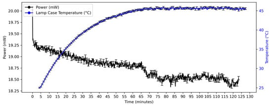
Figure 1. Variation in power output and case temperature of light source. After a 30 min warmup period, the drift in power between 30 and 120 min was 2.6%.

A Thorlabs fiber coupled spectrophotometer CCS200/M with a spectral resolution of 0.25 nm and a wavelength range from 200 to 1100 nm was used. Both the illumination and collection fibers had a core diameter of 550 µm and a numerical aperture (N.A) of 0.22. The two windows of the probe were made of a modified soda lime glass, i.e., silica (silicon dioxide SiO₂), soda (sodium oxide Na₂O), and lime (calcium oxide CaO). The following improvements were made to the optical components in this work. A corrugated plastic coil was used to protect the optical fibers. The fiber length was extended from 1 to 5 m to allow the electrical cabinet to be placed at a greater distance from the reactor. The power at the end of each fiber was measured. In going from a 1 m to a 5 m fiber, the power decreased by 0.23%. This corresponded to a fiber attenuation of 0.0025 dB per m.

Probe

The probe is designed to operate from 0 to 100 °C and is resistant to chemical compounds and corrosion. One of the improvements to the probe that was made in this version was to change the probe’s material from stainless steel 304 to stainless steel 316Ti for greater durability and resistance to corrosion. The following tests were performed. Firstly, a test at high temperature was carried out. The probe was immersed in distilled, deionized water and then heated to 100 °C before reaching the boiling point. The probe was held at this temperature for 2 h. Afterwards, a visual inspection of all parts was carried out to confirm that there was no damage. Secondly, a test for compatibility with sulfuric was performed. The probe was immersed in a solution of water and sulfuric acid with a pH of 2.0 for 170 h. Afterwards, a visual inspection was performed to determine that no damage occurred. Thirdly, the probe was immersed in a solution of highly concentrated 96% sulfuric acid for 2 h. Again no corrosion was seen on the external parts of the probe. In addition to this external visual inspection, a spectrum of distilled, deionized water was taken to ensure that the internal parts of the probe had not been affected.

Customizable attachments to mount the probe in reactors of different sizes were developed. Figure 2a shows the probe and the extension tubes for the 6 L reactor and Figure 2b shows those for the 160 L reactor.

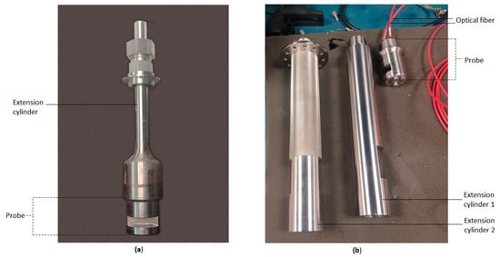
Figure 2. Probe and extension cylinder(s) to mount probe in (a) 6 L and (b) 160 L reactors.

Optical Calibration

Calibration and verification of the optical components in the Visum PSA system were carried out and compared to the manufacturer’s specifications to check for conformity. In addition, checks for conformity with our internal specifications for the probe were performed. The following tests were carried out. The ends of the illumination and collection fibers were inspected using a fiber inspection scope. The power output of the light source at the end of the illumination fiber was measured as described in the Optical Components Section. The following tests to characterize the spectrophotometer were performed: measurement of the wavelength calibration, spectral resolution, signal-to-noise (SNR) ratio, photo-linearity, and stability over time.

The probe is a modular device consisting of different parts. Its two windows were cleaned with lens tissue soaked in ethanol. During assembly of the probe, the power at various points was measured and compared to our internal specifications. These included the power incident on the first window of the probe, the power transmitted through the second window, and the power detected at the end of the collection fiber. With the probe assembled and positioned in air, the spectrum of light it transmitted was measured by the spectrophotometer. The probe was then placed in distilled, deionized water, and further spectra were taken. These were compared to our reference spectra for air and water for the probe. The probe was left in water for 2 days, during which spectra were acquired continuously. This test was carried out to check that the probe was waterproof. Any water leaking into the device leads to a decrease in the number in the transmitted light spectrum counts, making it easily detectable.

2.2.2. Software Description

The software consists of

• A user interface for acquiring spectra of transmitted light intensity versus wavelength;
• A real-time display of spectra of turbidity versus wavelength;
• A real-time display of the evolution of the estimated particle size during the synthesis.

2.2.3. Chemometric Model

Model Description

The Visum PSA system incorporates a chemometric model to estimate the particle size in real time from turbidity spectra measured during synthesis. The model is based on Partial Least Squares (PLS) regression [23], a multivariate statistical technique that establishes a predictive relationship between the turbidity spectra (input, X) and particle size (output, Y). PLS works by extracting latent variables (also called components) from the spectral data that capture the most relevant information for predicting the response variable—in this case, the particle size. Unlike other dimensionality reduction methods, such as principal component analysis (PCA) [24], PLS focuses on components that are maximally correlated with the response rather than solely maximizing variance in the predictors.

The PLS algorithm, designed for modeling a single response variable, was applied to the pre-processed spectral data. The model was built and trained using datasets collected from defined reactions, and subsequently validated on independent runs by comparing the predicted and measured particle size values. This procedure confirmed the model’s robustness and accuracy in both calibration and validation phases, demonstrating its reliability for real-time particle size prediction.

Data Preprocessing, Model Training, and Validation Design

To ensure model accuracy and robustness, only turbidity spectra corresponding to chemically relevant stages of the reaction were used. These spectra were pre-processed to eliminate external fluctuations and corrected to minimize spectral interferences. Outliers were identified and removed prior to modeling.

All spectra were mean-centered before model building. Other preprocessing techniques (such as SNV, smoothing, and derivative filters) were also evaluated. However, considering the specific nature of the turbidity-based spectroscopic data, the mean-centering approach alone yielded satisfactory results. Model training and optimization were performed using cross-validation (CV) with a Venetian blinds approach. Once satisfactory performance metrics were achieved, the finalized model was applied to external validation datasets composed of new acquired samples to evaluate prediction accuracy against known reference values. The good agreement between predicted and measured particle size confirm the reliability and generalizability of the model. Therefore, no additional preprocessing steps were deemed necessary.

For each reaction, the measured particle size values were temporally aligned with the corresponding turbidity spectra to create the calibration dataset. The temporal alignment algorithm is detailed in Appendix A. A PLS model was then built using this paired dataset, with the optimal number of latent variables determined by minimizing cross-validation error.

Model Application and Transferability

Once trained, the model was applied to predict particle size in new runs of the same reaction and in scaled-up processes, such as transferring a model developed in a 6 L reactor to a 160 L reactor. Additionally, a combined model using calibration data from two reactions with different kinetic profiles was successfully applied to a third reaction without additional calibration, demonstrating robustness and transferability across process conditions and reactor sizes.

This chemometric approach eliminates the need for explicit knowledge of the particles’ optical properties, relying instead on empirical correlations between scattering spectra and particle size. It thus enables fast, flexible, and scalable monitoring of nanoparticle synthesis.

2.3. Experimental Procedures for Acquiring Data During a Reaction

2.3.1. Installation of Probe in Reactor

The probe was attached to the end of the extension tube(s), specifically designed for the reactor, and then inserted into the reactor. The extension tube was lowered to a height so that the measuring gap in the probe was completely filled by the fluid level in the reactor. The tube was then clamped to the reactor. The radial position of the probe was such that it did not interfere with the motion of the reactor’s rotor blade(s).

2.3.2. Experimental Procedures for Measuring Turbidity During Reaction

Acquisition of Dark Spectrum $I_D\left(\lambda \right)$ for Turbidity Monitoring

The first spectrum that is taken at the start of any synthesis is the dark spectrum with the light source switched off. This is then subtracted from all future spectra by using the dark correction function of the spectrophotometer’s software (ThorSpectra software. GUI Version 3.20.8897.709. Lib Version 3.20).

Acquisition of Reference Spectrum $I_0\left(\lambda \right)$ for Turbidity Monitoring

The transmittance $T$ of the nanoparticle suspension at wavelength $\lambda$ is calculated by

$$T(\lambda )={\displaystyle \frac{I\left(\lambda \right)}{I_0\left(\lambda \right)}}$$

(1)

where $I_0$ is the intensity of the incident beam, and $I$ the intensity of the transmitted beam.

The turbidity $\tau$ of the suspension at wavelength $\lambda$ is calculated by

$$\tau (\lambda )={\displaystyle \frac{1}{L}}\ln \left[{\displaystyle \frac{I_0\left(\lambda \right)}{I\left(\lambda \right)}}\right]={\displaystyle \frac{1}{L}}\ln \left[{\displaystyle \frac{1}{T\left(\lambda \right)}}\right]$$

(2)

where $L$ is the optical path length of the beam traveling in the forward direction through the suspension in the gap in the probe. $L$ is given by the gap length, 1 cm.

From Equation (1), a reference spectrum of the incident intensity $I_0\left(\lambda \right)$ is needed to obtain $\tau \left(\lambda \right)$. This is taken once the reactor has been filled to its pre-fill level and before the reaction has been initiated. However, as seen in Figure 1, there is a small drift in the lamp’s power output over time. This translates to a variation in $I_0\left(\lambda \right)$ over time. So it is not sufficient to take just one reference spectrum at the start of the synthesis and use it in all calculations of $\tau \left(\lambda \right)$. The variation in $I_0\left(\lambda \right)$ over time was thus measured, as shown in Figure 3. A set of reference spectra $I_{0t}\left(\lambda \right)$ as a function of the time $t$ since the start of the reaction was thus obtained. After the 30 min warmup period, the drift in $I_{0t}\left(\lambda \right)$ over the next 90 min was found to be 3.2%. This is very similar to the variation in the lamp’s output power shown in Figure 1, as one would expect.

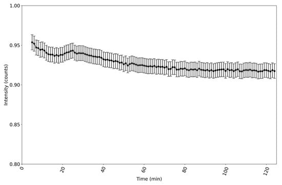
Figure 3. Variation in incident intensity $I_{0t}$ (λ) over time. The counts are those at 565 nm. After the 30 min warmup period, the drift in power between 30 and 120 min was 3.2%. The graph has a very similar form and drift to that shown in Figure 1, as one would expect, given that the same light source was used for each graph.

A spectrophotometer integration time of 4 ms per spectrum was chosen, as it gave a measured incident intensity at the peak wavelength of 565 nm corresponding to approximately 95% of the maximum number of counts that the spectrometer could measure, as can be seen in Figure 3. Once the reaction begins and particles start to form, scattering light, the transmitted intensity drops. Hence, it is best to use an integration time that gives a high initial number of counts.

Acquisition of Transmitted Spectra $I\left(\lambda \right)$ for Turbidity Monitoring

Based on Equation (1), a spectrum of the light transmitted by the suspension $I\left(\lambda \right)$ is needed to obtain $\tau \left(\lambda \right)$. Upon adding the first component to the reactor, the acquisition of transmitted spectra $I\left(\lambda \right)$ was initiated. A set of transmitted spectra $I_t\left(\lambda \right)$ as a function of $t$ was obtained. The transmittance $T_t\left(\lambda \right)$ and turbidity ${\tau }_t\left(\lambda \right)$ at each time $t$ were obtained by using the transmitted spectra $I_t\left(\lambda \right)$ and reference spectra $I_{0t}\left(\lambda \right)$ in Equations (1) and (2).

The software was configured to record a spectrum every 10 s until the reaction gelation point, identified by observing the suspension in the reactor, was reached. At this point, the suspension was too turbid and the transmitted intensity too low to be measured. During the reaction, the software displayed the turbidity spectrum $\tau \left(\lambda \right)$.

2.3.3. Procedure for Sampling Volumes of Nanoparticle Suspension for Measuring Particle Size

During the synthesis, the following procedure was implemented to obtain a sample volume of the nanoparticle suspension for the purpose of measuring the particle size, as described in the next section. A glass beaker held in a support with long handles was used to allow the reactor operator to take samples from the hot reactor while remaining at a safe distance from it. The operator put on thermal gloves, opened the reactor lid, lowered the beaker into the reactor to collect some of the suspension, lifted the beaker out of the reactor, and closed the reactor lid. The operator then decanted 5 mL of the suspension from the beaker into a cuvette. A sample was removed from the reactor every 5 min until the suspension became a gel.

2.3.4. Experimental Procedure for Measuring Particle Size During Synthesis Reaction

The particle size reference values needed for the model development were measured during the synthesis using a Zetasizer Nano ZS DLS instrument (Malvern Panalytical, Malvern, UK). Although the sample had been taken out of the reactor, the reaction still continued in the cuvette. In an effort to slow down the reaction and thus ensure that the suspension to be placed in the DLS instrument was in as similar a state as possible to that in the reactor, the cuvette was placed in an ice bath. When the sample temperature had fallen to 25 °C, it was assumed that the particle size would remain approximately constant from then onwards. The cuvette was thus placed in the DLS instrument. A total of 5 runs (or measurements) were performed, each with a scan time of 2 s per repeat. The time per repeat was therefore 10 s, and 3 repeats were performed. The time to complete the 3 repeats was therefore 0.5 min. The steps performed from taking the sample out of the reactor to completing the particle size measurement are described in Table 1.

Table 1. Actions and times to measure particle size during synthesis reaction.

Start Time (min)	Action	Time to Complete Action (min)	Total Time Elapsed (min)
0	Walk from the reactor with the sample in the cuvette to the DLS room	0.5	0.5
0.5	Cool the sample cuvette in an ice bath to 25 °C in order to stabilize the sample	1.5	2.0
2.0	Place the cuvette in the DLS instrument, set the number of repeats, number of runs per repeat, and scan time per run and name the measurement	0.5	2.5
2.5	DLS instrument executes optimization stage, where the cuvette position, compensation, and attenuator settings for the cuvette are determined	1.0	3.5
3.5	DLS instrument performs the 3 repeats	0.5	4.0

Total time = 4 min.

If we consider a sample removed from the reactor at time $t=t_0$, the particle size measurement obtained is actually an estimate of the particle size at time $t=t_0+2$ (not $t_0+$4) minutes because this is when it was assumed that the growth outside the reactor had stopped. The measurement is an overestimate of the true particle size in the reactor at time $t=t_0,$ as growth has occurred outside the reactor. This will be corrected for, as explained in Section 2.3.5 and Appendix A.

The samples at all sampling times had a low polydispersity index (PDI), <0.4. For this reason, the z-average parameter was used for the particle size of the samples.

2.3.5. Experimental Procedure for Estimating Growth in Particle Size Outside Reactor

As noted in Section 2.3.4, particle growth occurs outside the reactor. Particle size measurements are also obtained with a time lag with respect to the state of the suspension in the reactor. These points need to be addressed in order for the model to make accurate predictions of the particle size inside the reactor. The procedure for doing so, i.e., for estimating the ex-reactor growth and aligning the correct turbidity spectrum to the particle size, is described in Appendix A.

This procedure requires an estimate of the growth in the particle size outside the reactor in order to work backwards and obtain an estimate for the particle size at time $t=t_0$. To obtain the data needed for the estimate, the following method was employed. During a test synthesis run, samples were removed from the reactor every 5 min, as described in Section 2.3.4. However, in this run, the protocol for measuring the particle size was altered with respect to that in Section 2.3.4. The change made was that the samples were not placed in the ice bath. This allowed the reaction in the cuvette to continue outside the reactor, thus enabling us to obtain an estimate of the particle growth outside the reactor by measuring the particle size every 0.5 min for a total of 2.5 min. The steps performed, from taking the sample out of the reactor to completing the particle size measurement, are described in Table 2.

Table 2. Actions and times to measure particle size for the purpose of estimating growth in the particle size outside reactor.

Start Time (min)	Action	Time to Complete Action (min)	Total Time Elapsed (min)
0	Walk from the reactor with the sample in the cuvette to the DLS room	0.5	0.5
0.5	Place the cuvette in the DLS instrument, set the number of repeats, number of runs per repeat, and scan time per run and name the measurement	0.5	1.0
1.0	DLS instrument executes optimization stage, where the cuvette position, compensation, and attenuator settings for the cuvette are determined	1.0	2.0
2.0	DLS instrument performs the 3 repeats for the measurement at time t = t0 + 2.5	0.5	2.5
2.5	DLS instrument performs the 3 repeats for the measurement at time t = t0 + 3.0	0.5	3.0
3.0	DLS instrument performs the 3 repeats for the measurement at time t = t0 + 3.5	0.5	3.5
3.5	DLS instrument performs the 3 repeats for the measurement at time t = t0 + 4.0	0.5	4.0
4.0	DLS instrument performs the 3 repeats for the measurement at time t = t0 + 4.5	0.5	4.5

Total time = 4.5 min.

A total of 5 data points of particle size outside the reactor versus time were obtained. The way in which these data points were used is explained in Appendix A.

2.3.6. Procedure for Quenching, Cooling, and Cleaning Reactor at End of Reaction

At the end of the synthesis reaction, the reactor lid was opened. The reactor was quenched by pumping cooling water through the jacket around the reactor. Diluted sulfuric acid was added to reduce the pH to 6.7. This did not affect the size of the nanoparticles synthesized in the gel but made it easier to remove the gel. The gel was drained out of the reactor. The first cleaning cycle was initiated. The residual gel left on the reactor’s rotor blades, the Visum PSA probe, and the reactor’s sides was washed off by holding a jet spray water gun near the open lid and pointing it at the rotor blades, probes, and sides of the reactor. A volume of cleaning water, 40 L in the case of the 160 L reactor, was pumped into the reactor. The reactor’s rotor blades were set in motion to circulate this water around the reactor. Then, the water was drained out of the reactor. A second identical cleaning cycle was performed. The quenching and cleaning process took approximately 50 min for the 160 L reactor, after which the reactor could be used for a new synthesis procedure.

2.3.7. Procedure for Maintenance and Fouling Checks

In each synthesis, some nanoparticles accumulated on the probe and, more importantly, on its two windows. As part of the cleaning procedure, described in Section 2.3.6, the jet spray water gun was directed at the probe’s windows to remove as many nanoparticles as possible. Nevertheless, some particles accumulated on the windows. Their effect was to reduce the transmission of light through the probe. The build-up of particles on the windows can be evidenced by observing the evolution over time of $I_0\left(\lambda \right)$ from one run to the next. As particles built up, $I_0\left(\lambda \right)$ decreased. It was decided that when $I_0\left(\lambda \right)$ had fallen to 90% of its value measured in the first run, the probe should be removed from the reactor and the windows thoroughly cleaned using lens tissue soaked in ethanol. It was found that for the longer reaction, reaction B, which took up to 80 min, the probe had to be removed, and its windows cleaned after every 5 syntheses.

3. Results and Discussion

3.1. Turbidity and Light Scattering by Silica Nanoparticles

The turbidity versus wavelength curve is very similar for the three reactions. Therefore, only the curve for reaction B is shown (Figure 4). The form of the curve can be explained in terms of light scattering by particles. For the entire reaction, except for very close to the gelation point, the particle diameter was small, at <10% of the wavelength of the incident light. Scattering of light by spherical particles of this size can be described by Rayleigh scattering theory [25]. However, previous studies [26] have shown that silica particle aggregates are fractal. Additionally, the ratio of the refractive indices of silica, 1.44, and water, 1.33, is close to 1. The last two considerations imply that Rayleigh Gans Debye (RGD) theory [27] describes more accurately the light scattering by the silica nanoparticles in this study. The theory predicts a decrease in the intensity of scattered light and thus the turbidity as the wavelength increases, as can be seen in Figure 4. Optical models describing the scattering of light by fractal aggregates [28] have been developed to relate the turbidity to the size and geometrical form of the aggregate. In this work, though, the model employed was chemometric rather than optical.

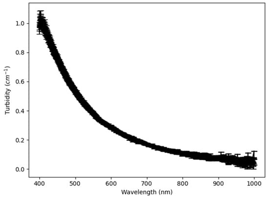
Figure 4. Graph of turbidity versus wavelength at time 55 min in 160 L reactor for reaction B. The decrease in turbidity with wavelength is consistent with RGD theory.

3.2. Turbidity, Particle Agglomeration, and Gelation in Silica Nanoparticle Synthesis Reactions

In general, in silica nanoparticle syntheses using neutralization of a sodium silicate solution, the silica particles at the start of the reaction are small, with a diameter of <10 to 15 nm. These are referred to as primary particles. As the primary particles are small compared to the wavelength of light, they scatter little light, and the turbidity of the suspension is low. Their electric charge is low, so they do not repel each other. Instead, they coagulate to form aggregates. As the reaction progresses, the aggregates become progressively bigger and scatter more light. The suspension thus becomes more turbid. At some point during the synthesis, a large proportion of all the precipitated silica forms a large agglomerated, highly turbid mass or gel. This point is called the gelation point and signals the end of the reaction.

3.3. Turbidity Monitoring and Particle Size Prediction in the Three Reactions Studied

The three reactions A, B, and C, took, respectively, about 24, 65, and 35 min, with some small time variations between runs. All three exhibited a slow growth in particle size (Figure 6, Figure 9 and Figure 12) for the majority of the reaction, followed by a sharp increase in the final few minutes. The aggregation of the particles during the reaction was thus non-linear. The turbidity of the suspensions (Figure 5, Figure 8 and Figure 11) followed the same trend as the particle size. The results for the three reactions are described in the following three sub-sections.

3.3.1. Reaction A

Turbidity Measurements in 160 L Reactor

The variation in the turbidity of the suspension with time since the start of the reaction in the 160 L reactor is shown for three reaction runs in Figure 5. The turbidity increased slowly until around 22 min. From then on, it increased sharply. The gelation point was reached soon after, at around 24 min. The evolution of the turbidity with time was very similar for the three runs, showing high repeatability of the reaction in the 160 L reactor.

Figure 5. Evolution of measured turbidity in 160 L reactor for synthesis of silica nanoparticles by reaction A. The turbidity values are those at 565 nm. Data are plotted as a function of time since the start of the reaction. All runs show a slow initial increase in turbidity, followed by a rapid increase to a turbidity of ≈ 6 cm⁻¹ in the last 2 min of the reaction.

Particle Size Measurements in 160 L Reactor

The variation in the particle size with time is presented in Figure 6. In the first 10 min of the reaction, the particles had barely formed and were too small to be measured reliably by the DLS instrument. From 10 min onwards, particles began to aggregate, and the size of the aggregates increased. Similarly to Figure 5, a steep increase in particle size occurred after around 20 min. The particle size at the gelation point was in the order of 240 to 260 nm. Very similar particle sizes were observed at corresponding times in the three runs, confirming the high reproducibility of the reaction in the 160 L reactor.

Figure 6. Evolution of z-average particle size during synthesis of silica nanoparticles as measured by DLS for three independent runs (run 1: black; run 2: green; run 3: blue) of reaction A in 160 L reactor. Data are plotted as a function of time since the start of the reaction. All runs show a similar growth profile with an initial lag phase up to ~15 min, followed by a rapid increase in particle size leading to values above 250 nm near 25 min.

The chemometric model for reaction A was developed using the turbidity and particle size data for the three runs. The reaction was then run for a fourth time, during which turbidity and particle size data were collected. The turbidity data from this run was used as input to the model. The model was used to predict the variation in the particle size as a function of time. A comparison with the measured particle size is presented in Figure 7.

Figure 7. Evolution of z-average particle size during synthesis of silica nanoparticles as measured by DLS, predicted particle size, and residual for the fourth run of reaction A in the 160 L reactor. Data are plotted as a function of time since the start of the reaction. The residual was about 2 to 3 nm at 10, 15, and 25 min, but 18 nm at 20 min. Slower particle growth from 15 to 20 min occurred in this run compared to the other three runs. Inset: measured and predicted particle size at discrete times.

The inset in Figure 7 shows a strong correlation between the measured particle size and the model’s predictions for reaction A in the 160 L reactor. The difference between the measured and predicted particle size, the residual, was in the order of 2 to 3 nm at 10, 15, and 25 min, but for the measurement at 20 min, it was 18 nm. Looking at the DLS data for run 4, the measurement of the particle size at 20 min in this run was 7 nm lower than in run 1, 17 nm lower than in run 2, and 23 nm lower than in run 3. This indicates that it was an outlier. It is apparent that from 15 to 20 min, the reaction advanced more slowly in this run than in the other three runs, and hence, the particle size was lower at 20 min.

3.3.2. Reaction B

Turbidity Measurements in 6 L and 160 L Reactors

Figure 8 displays the variation in the turbidity of the suspension with time since the start of the reaction in the 6 L and 160 L reactors. Three reaction runs are displayed for each reactor. For the 6 L reactor, the turbidity increased slowly until around 65 min. Thereafter, a rapid increase is observable. The gelation point was reached soon after. This occurred at about 75 min into the first run, whereas in the second and third runs, the gelation point was reached at about 80 min. The reaction thus proceeded more quickly in the first run.

Figure 8. Evolution of measured turbidity in 6 L and 160 L reactors for synthesis of silica nanoparticles by reaction B. The turbidity values are those at 565 nm. Data are plotted as a function of time since the start of the reaction. Data for individual runs are shown in light colors, while the data for the mean of the runs are shown in a darker colors. Runs in the 6 L reactor show a slow increase in turbidity until 65 min, followed by a rapid increase to a turbidity of ≈ 6 cm⁻¹ in the last 10 min of the reaction. Runs in the 160 L reactor show a slow increase until 55 min, followed by a rapid increase to a turbidity of ≈ 6 cm⁻¹ in the last 10 min. The reaction proceeded more quickly in the 160 L reactor.

For the 160 L reactor, the turbidity increased slowly until around 55 min. Thereafter, a rapid increase occurred. The gelation point was reached at about 61 min in the first run, 64 min in the second run, and 65 min in the third run. Therefore, there was a small difference in the reaction rate among the three runs. Considering all six runs, we conclude that the gelation point occurs at a turbidity of 6 cm⁻¹ in our system.

If we compare the change in turbidity with time for reaction B in the two reactors, we notice that the gelation point was reached at about 10 to 15 min sooner in the larger reactor. This was due to two factors: (1) a more homogeneous mixing of components is generally obtained in larger reactors; (2) in the smaller reactor, the concentrated sulfuric acid was added at a constant rate throughout the reaction, whereas in the larger reactor, its dosing rate was continually adjusted in order to keep the pH constant throughout the reaction.

Particle Size Measurements in 6 L and 160 L Reactors

The variation in particle size over time in the 6 L and 160 L reactors is shown in Figure 9. For the 6 L reactor, the particles were too small to be measured reliably by DLS in the first 25 min of the reaction. From this moment onwards, particles began to aggregate. As shown in Figure 8, a steep increase was observed after 60 min, as the particles aggregated rapidly. In the first run, the particle size at 70 min was in the order of 320 nm. In the second and third runs, it was 200 and 220 nm, respectively. The first run occurred more quickly, as also seen in the evolution of the turbidity in Figure 8, and so a greater particle size was reached after the same length of time.

Figure 9. Evolution of z-average particle size during synthesis of silica nanoparticles as measured by DLS for reaction B in the 6 L and 160 L reactors. Data are plotted as a function of time since the start of the reaction. Runs in the 6 L reactor show a slow increase in growth until 60 min, followed by a rapid increase in particle size, leading to values greater than 200 nm at 70 min. Runs in the 160 L reactor show a slow increase in growth until 50 min, followed by a rapid increase in particle size, leading to values greater than 150 nm at 60 min.

For the 160 L reactor, the particles were large enough to be measured by DLS from 15 min onwards. A sharp rise in the particle size was seen after 50 min. The particle size at 60 min was in the order of 235 nm in the first run, 150 nm in the second run, and 160 nm in the third run. The first run proceeded at a higher rate, as also apparent in the evolution of the turbidity in Figure 8, leading to a larger particle size after the same length of time.

In both reactors, the particle size measurements stopped at about 5 min before the end of the reaction as the PDI exceeded 0.7, indicating that the particle size distribution in the sample was broad and not well described by the z-average parameter [29].

Application of Model Developed for 6 L Reactor to 160 L Reactor

The chemometric model for reaction B was built using the turbidity and particle size data acquired for the three runs in the 6 L reactor. It was applied to the third run of the same reaction in the 160 L reactor. The turbidity data acquired for the third run of reaction B in the 160 L reactor was used as the input to the model. The measured particle size and the model’s predicted particle size are shown in Figure 10.

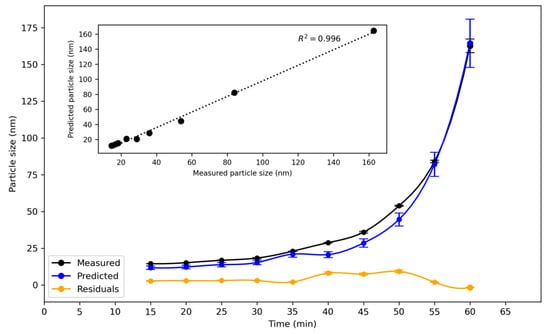
Figure 10. Evolution of z-average particle size during synthesis of silica nanoparticles as measured by DLS, predicted particle size, and residual for third run of reaction B in 160 L reactor. Predictions were made by the model built from data for the 6 L reactor. Data are plotted as a function of time since the start of the reaction. The residual was about 2 to 3 nm from 15 to 35 min, rising to a maximum value of 9 nm at 50 min. Inset: measured and predicted particle size at discrete times.

The residual was in the order of 2 to 3 nm from 15 to 35 min. It reached a maximum value of 9 nm at 50 min. The average relative % difference between the measured and predicted particle size over the whole run was 16%, which is a good result given that the data acquired to create the model and that used to validate it originated from reactors of significantly different volumes. Reaction B also finished about 10 to 15 min quicker in the larger reactor. Nevertheless, the model, created from experimental data in the smaller reactor, was able to reasonably estimate the particle size in the larger reactor. This finding demonstrates the transportability of the chemometric model for reaction B from one set of reaction conditions in the smaller reactor to a different set of reaction conditions in the larger reactor.

As with any predictive model, the greater the quantity of input data, the more accurate the model’s predictions. On that point, we acknowledge that the model would be more complete if there were more particle size measurements in the 5 min period of rapid turbidity increase near the end of each reaction, which leads to the gelation point. While the Visum PSA system is able to directly measure the turbidity on this fast-changing timescale, the evolution of the actual particle size during this period is less understood. The limiting factor that prevented more measurements in this period was the overall time required to perform a particle size measurement, as described in Section 2.3.4.

3.3.3. Reaction C

Turbidity Measurements in 160 L Reactor

The variation in the turbidity of the suspension over time in the 160 L reactor is shown for three reaction runs in Figure 11. The turbidity increased slowly until around 32 min. From that point onwards, it increased steeply. The gelation point was reached at about 36 min in the first and third runs, and at about 37 min in the second run.

Figure 11. Evolution of measured turbidity in the 160 L reactor for synthesis of silica nanoparticles by reaction C. The turbidity values are those at 565 nm. Data are plotted as a function of time since the start of the reaction. All runs show a slow increase in turbidity until 32 min, followed by a rapid increase to a turbidity of ≈6 cm⁻¹ in the last 5 min of the reaction.

Particle Size Measurements in 160 L Reactor

Figure 12 illustrates the change in the particle size, with time in the 160 L reactor. The first reliable particle size measurements occurred 20 min into the reaction. The particle size rose quickly after about 30 min in the three runs. In the first run, the particle size at the gelation point was in the order of 190 nm; in the second run, 215 nm; and in the third run, 260 nm.

Figure 12. Evolution of z-average particle size during synthesis of silica nanoparticles as measured by DLS for three independent runs (run 1: black; run 2: green; run 3: blue) of reaction C in 160 L reactor. Data are plotted as a function of time since the start of the reaction. All runs show a similar growth profile with initial slow growth up to 30 min, followed by a rapid increase in particle size, leading to values above 190 nm near 35 min.

Application of Combined Model Developed for Reactions A and B to Reaction C in 160 L Reactor

A combined chemometric model for reaction C was created from the two models previously described. These included the model developed for reaction A using turbidity and particle size data acquired in the 160 L reactor and the model built for reaction B using data acquired in the 6 L reactor. Using turbidity data acquired for reaction C in the 160 L reactor as the input to the combined model, the model was employed to estimate the particle size in reaction C. No measured particle size data for reaction C was obtained previously for input into the model. Figure 13 displays a comparison of the measured and estimated particle size.

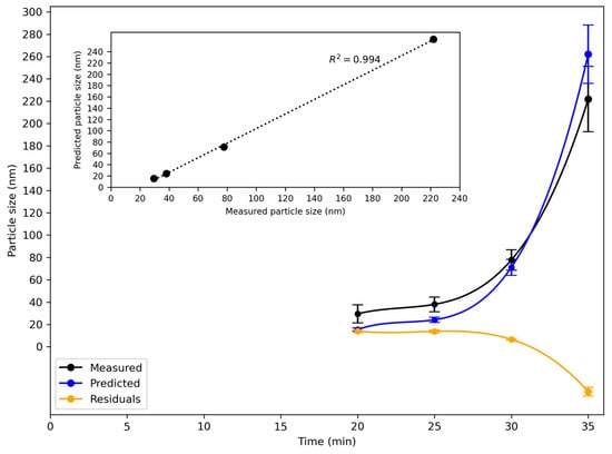
Figure 13. Evolution of z-average particle size during synthesis of silica nanoparticles as measured by DLS, predicted particle size, and residual for the average of the three runs for reaction C in 160 L reactor. Data are plotted as a function of time since the start of the reaction. Predictions were made by a composite model, based on the model developed for reaction A using data from the 160 L reactor and the model built for reaction B using data from the 6 L reactor. The residual varied from 6 to 14 nm between 20 and 30 min, with a larger residual close to the gelation point. Inset: measured and predicted particle size at discrete times.

The residual was approximately 14 nm at 20 and 25 and 6 nm at 30 min. The reaction rate increased very steeply from 32 min onwards towards the gelation point, as shown in the turbidity graph in Figure 11. The predictions of particle size using the composite model were less accurate in this time region, and the residual increased. An average relative % difference between the measured and predicted particle size over the whole run of 18% was found, which shows reasonably good agreement between the two. This result demonstrates that it is possible to combine chemometric models for two similar reactions, differing in reaction rate and carried out in different-sized reactors, into a single, combined model. It also proves that this model can make reasonably accurate predictions of particle size in a third similar reaction that proceeds at a different rate, even though no data for input into the model has been previously acquired for the third reaction.

The Visum PSA system can, in principle, be used to monitor other nanoparticles, as its underlying physical principle—that of measuring the light transmitted by a suspension of scattering particles—occurs in all nanoparticle suspensions. In practice, though, it is recommended to test the system first with the particular nanoparticle that one wishes to measure. This is because some nanoparticles have a greater tendency to accumulate on the probe’s windows than others, leading to reduced light transmission. The rate of accumulation depends both on the properties of the nanoparticle and the probe’s windows. To that end, we are investigating different materials for the windows, which minimize the sticking of different, commonly synthesized nanoparticles.

4. Conclusions

In this work, we have described a system, the Visum PSA system, for the in-line, real-time monitoring of nanoparticle synthesis by turbidity measurement and chemometric modeling. The system was used to measure the turbidity and to estimate the particle size for three industrial silica nanoparticle synthesis processes, run in reactors with volumes of 6 L and 160 L. The reaction components and synthesis procedure were the same for all three reactions, but the doping speeds were different, giving three different reaction end times. In the three reactions studied, a slow increase in particle size and, therefore, turbidity, was observed for most of the reaction until a sharp increase in particle aggregation occurred in the last three to five minutes.

The system’s turbidity monitoring capability provided information on a sub-minute temporal resolution of the reaction progress and gave a clear indication of when the gelation point was reached. This occurred at a turbidity value of 6 cm⁻¹ in our system. Variations in the end time of the reaction from one run to the next were therefore identified by the system, which allowed the reaction to be stopped at the appropriate moment. The system’s predictive model was shown to provide accurate predictions of the evolution of the particle size during the reactions. Of particular interest is that the model developed for a reaction in the smaller, 6 L reactor was applied to the same reaction in the larger, 160 L reactor and resulted in particle size estimates that differed, on average, by 16% from the measured particle sizes. Also of importance is how the combined model built from the first two reactions was successfully used to predict the particle size in the third reaction without first having to acquire any data for the third reaction to go into the model. In this case, an average relative difference of 18% between the measured and predicted particle size was found. These results illustrate the transferability of the predictive model from one size of reactor to the next and from one version, i.e., one doping speed of the same reaction, to the next. Models can therefore be developed cost-efficiently in small, low-cost reactors with small quantities of components and then applied to monitor synthesis reactions in larger, more expensive reactors.

The upscaling potential of the system was evident, as it was used equally successfully to monitor reactions in an industrial, high-throughput 160 L reactor as in a small, research laboratory 6 L reactor. Only the mechanical components needed to mount the probe in the specific reactor had to be adapted. Despite the presence of highly concentrated acids at a high temperature of 90 °C in the reactor, the probe operated reliably and remained free from corrosion. In summary, the Visum PSA system could be a valuable system for providing real-time information about the reaction progress and particle sizes in industrial nanoparticle syntheses occurring in harsh reaction conditions.

Appendix A.1. Definition of Variables

We define the following variables:

$t$ is the time since the start of the reaction. This is also the time at which the turbidity spectrum is recorded.

${\tau }_t$ is the turbidity spectrum recorded in the reactor at time $t$. This is a 2D dimensional matrix consisting of the turbidity at various wavelengths.

$d_t$ is the particle size inside the reactor at time $t$. This is the parameter that we wish to find.

$d_{te}$ is the estimated particle size inside the reactor at time $t$. The subscript e stands for “estimated”.

$t_s$ is the time since a sample was removed from the reactor for a particular particle size measurement.

Appendix A.2. Difference in Time Between Recorded Turbidity Spectrum and Measured Particle Size

The procedure described in this Appendix is needed for the following reasons. As noted in the Acquisition of Transmitted Spectra $I\left(\lambda \right)$ for Turbidity Monitoring Section, the turbidity spectrum of the nanoparticle suspension inside the reactor is recorded every 10 s while the particle size is measured only every 5 min. In addition, the particle size measurement is performed outside the reactor where growth continues until it is prevented by cooling to 25 °C in an ice bath. The measurement also takes a certain amount of time, as described in Section 2.3.4. The recorded turbidity spectrum and the measured particle size therefore relate to different states of the nanoparticles and at different times. We wish to correct for this as best we can so that we have a matching set of particle size values and turbidity spectra for the synthesis.

Appendix A.3. High-Level Steps to Create Calibration Dataset

The high-level steps to create the set are as follows:

• Populate a table with values of time $t$, recorded turbidity spectra ${\tau }_t,$ and particle sizes $d_t$.
• Obtain values for the particle size $d_t$ at intermediate times.
• Calculate an estimate $d_{te}$ for what the particle size actually would have been at the time $t$ at which the turbidity spectrum was recorded.
• Look up the particle size $d_t$ which most closely matches the estimated particle size $d_{te}$ in step 3.
• Align the correct turbidity spectrum ${\tau }_t$ to the particle size by shifting the turbidity spectra in time.
• Remove the columns for time and estimated particle size to create the calibration dataset.

Appendix A.4. Detailed Steps to Create Calibration Dataset

We used the 5 min time interval from $t$ = 10 to 15 min and the particle size measurement at $t$ = 15 min in one of the reactions to illustrate the population of the tables in the various steps. A schematic representation showing this interval in the tables is given in Figure A1. Only some of the rows corresponding to each 10 s interval at which the turbidity spectrum was measured are shown in order to avoid making the figure too big.

• Populate a table with values of time $t$, recorded turbidity spectra ${\tau }_t,$ and particle sizes $d_t$.

The values of time $t$, recorded turbidity spectra ${\tau }_t,$ and measured particle sizes $d_t$ for the complete run are used to populate Table 1, shown in Figure A1. We know from Section 2.3.4 that the particle size of the sample removed from the reactor at time $t$ = 10 min $d_{10}$ is more like an estimate of the size at time $t=10+2=$ 12 min than at $t$ = 10 min. Hence, we show $d_{10}$ in inverted commas in Figure A1 to indicate that this value is not really the particle size at $t$ = 10 min. Likewise, $d_{15}$ is closer to an estimate of the particle size at $t$ = 17 min than to the size at $t$ = 15 min, and so it is placed in inverted commas. At this stage, the table has a lot of entries for ${\tau }_t$ but few for $d_t$.

2.

Obtain values for the particle size $d_t$ at intermediate times.

We used cubic spline interpolation to find the 29 intermediate values of $d_t$ between ${”d}_{10}”$ and ${”d}_{15}”$ in the 5 min interval. We added these values to Table 1 to create Table 2, which now has values in every row.

3.

Obtain an estimate $d_{te}$ for what the particle size would have been at the time $t$ at which the turbidity spectrum was recorded.

We plotted a graph of the particle size outside the reactor versus the time since the sample was removed from the reactor $t_s$. The particles continued to grow in this time. The data points used are as follows:

• The point measured 2 min after the sample removal, as described in Section 2.3.4.
• Five points measured at 2.5, 3.0, 3.5, 4.0, and 4.5 min after the sample removal, as described in Section 2.3.5.

By fitting to the curve, we obtained a polynomial. The value of the coefficient giving the intercept with the y (i.e., the particle size) axis (i.e., at $t_s$= 0) provides an estimate of the particle size at the time the sample was removed from the reactor. This is equal to the time at which the turbidity spectrum was recorded. So, in our example, we obtained an estimate for the particle size $d_{15e}$ at time $t$ = 15 min.

4.

Look up the particle size in Table 2 that most closely matches the estimated particle size in step 3.

We looked up the particle size in the column $d_t$ whose value was closest to the estimated particle size $d_{15e}$ obtained in step 3. We placed $d_{15e}$ on the same row in a new column and called this Table 3. This row will correspond to an earlier time in the table for the following reason. In all the synthesis reactions, the particle size increased with time. So, seeing as $d_{15e}$ is smaller than ${”d}_{15}”$, it must be associated with an earlier time in the reaction. In the example given in Figure A1, we assume that the particle size in the row corresponding to time $t$ = 13 min ${”d}_{13}”$ is the closest to $d_{15e}$. However, this is just for the purposes of this example and depends on the data for the particular synthesis run.

5.

Align the correct turbidity spectrum to the particle size by shifting the turbidity spectra in time.

Currently, Table 3 shows that the turbidity spectrum in the row corresponding to the estimated particle size inside the reactor at time $t$ = 15 min $d_{15e}$ is the spectrum recorded at time t = 13 min rather than that at t = 15 min. Therefore, we shifted the turbidity spectra up in the table by a number of rows equal to this time difference—in this case, by 15 − 13 = 2 min. The turbidity spectra ${\tau }_t$ are now correctly matched to the particle sizes $d_t$ for the 5 min interval in this new table, Table 4. The uncertainty in time in the alignment procedure is estimated to be around 1 min. The procedure described in this section was carried out for all 5 min time periods in the reaction, starting with the last time period and going backwards in time, in order to complete Table 4.

6.

Remove the columns for time and estimated particle size to create the calibration dataset.

The model requires as input a turbidity spectrum acquired in a synthesis reaction rather than a time in order to predict the particle size. Hence, we removed the time and estimated particle size from Table 4 to obtain Table 5, the calibration dataset, shown in Figure A1.

Figure A1. Tables created during the construction of the calibration dataset. The 5 min time interval from 10 to 15 min in a reaction is used as an example. Only some of the rows corresponding to each 10 s interval at which the turbidity spectrum was measured are shown in order to keep the figure to a manageable size. Table 1 contains values of time $t$, recorded turbidity spectra ${\tau }_t$, and measured particle sizes $d_t$. Table 2 includes interpolated values of the particle size $d_t$ at intermediate times in the interval. Table 3 contains the estimate for what the particle size would have been at the time that the turbidity spectrum was actually recorded $d_{te}$ placed in the same row as the particle size whose value is closest to it, as indicated by the green arrow. Table 4 shows the turbidity spectra shifted in time and correctly aligned to the particle size. Table 5 shows the calibration dataset.

References

- Jenjob, R.; Phakkeeree, T.; Seidi, F.; Theerasilp, M.; Crespy, D. Emulsion Techniques for the Production of Pharmacological Nanoparticles. Macromol. Biosci. 2019, 19, 1900063. [Google Scholar] [CrossRef]
- Cho, Y.-S.; Ji, S.; Kim, Y.S. Synthesis of Polymeric Nanoparticles by Emulsion Polymerization for Particle Self-Assembly Applications. J. Nanosci. Nanotechnol. 2019, 19, 6398–6407. [Google Scholar] [CrossRef]
- Joni, I.M.; Rukiah; Panatarani, C. Synthesis of Silica Particles by Precipitation Method of Sodium Silicate: Effect of Temperature, pH and Mixing Technique. AIP Conf. Proc. 2020, 2219, 080018. [Google Scholar] [CrossRef]
- Zulfiqar, U.; Subhani, T.; Wilayat Husain, S. Synthesis of Silica Nanoparticles from Sodium Silicate under Alkaline Conditions. J. Sol-Gel Sci. Technol. 2016, 77, 753–758. [Google Scholar] [CrossRef]
- Ferreira, L.F.; Giordano, G.F.; Gobbi, A.L.; Piazzetta, M.H.O.; Schleder, G.R.; Lima, R.S. Real-Time and in Situ Monitoring of the Synthesis of Silica Nanoparticles. ACS Sens. 2022, 7, 1045–1057. [Google Scholar] [CrossRef] [PubMed]
- Meulendijks, N.; Van Ee, R.; Stevens, R.; Mourad, M.; Verheijen, M.; Kambly, N.; Armenta, R.; Buskens, P. Flow Cell Coupled Dynamic Light Scattering for Real-Time Monitoring of Nanoparticle Size during Liquid Phase Bottom-up Synthesis. Appl. Sci. 2018, 8, 108. [Google Scholar] [CrossRef]
- Besenhard, M.O.; Jiang, D.; Pankhurst, Q.A.; Southern, P.; Damilos, S.; Storozhuk, L.; Demosthenous, A.; Thanh, N.T.K.; Dobson, P.; Gavriilidis, A. Development of an In-Line Magnetometer for Flow Chemistry and Its Demonstration for Magnetic Nanoparticle Synthesis. Lab Chip 2021, 21, 3775–3783. [Google Scholar] [CrossRef]
- Pan, B.; Madani, M.S.; Forsberg, A.P.; Brutchey, R.L.; Malmstadt, N. Solvent Dependence of Ionic Liquid-Based Pt Nanoparticle Synthesis: Machine Learning-Aided in-Line Monitoring in a Flow Reactor. ACS Nano 2024, 18, 25542–25551. [Google Scholar] [CrossRef] [PubMed]
- Bolze, H.; Erfle, P.; Riewe, J.; Bunjes, H.; Dietzel, A.; Burg, T.P. A Microfluidic Split-Flow Technology for Product Characterization in Continuous Low-Volume Nanoparticle Synthesis. Micromachines 2019, 10, 179. [Google Scholar] [CrossRef]
- Zimmermann, S.; Reich, O.; Bressel, L. Exploitation of Inline Photon Density Wave Spectroscopy for Titania Particle Syntheses. J. Am. Ceram. Soc. 2023, 106, 671–680. [Google Scholar] [CrossRef]
- Häne, J.; Brühwiler, D.; Ecker, A.; Hass, R. Real-Time Inline Monitoring of Zeolite Synthesis by Photon Density Wave Spectroscopy. Microporous Mesoporous Mater. 2019, 288, 109580. [Google Scholar] [CrossRef]
- Tanguchi, J.; Murata, H.; Okamura, Y. Analysis of Aggregation and Dispersion States of Small Particles in Concentrated Suspension by Using Diffused Photon Density Wave Spectroscopy. Colloids Surf. B Biointerfaces 2010, 76, 137–144. [Google Scholar] [CrossRef]
- Schlappa, S.; Brenker, L.J.; Bressel, L.; Hass, R.; Münzberg, M. Process Characterization of Polyvinyl Acetate Emulsions Applying Inline Photon Density Wave Spectroscopy at High Solid Contents. Polymers 2021, 13, 669. [Google Scholar] [CrossRef]
- Aspiazu, U.O.; Hamzehlou, S.; Palombo Blascetta, N.; Paulis, M.; Leiza, J.R. Wavelength Exponent Based Calibration for Turbidity Spectroscopy: Monitoring the Particle Size during Emulsion Polymerization Reactions. J. Colloid Interface Sci. 2023, 652, 1685–1692. [Google Scholar] [CrossRef]
- Aspiazu, U.O.; Gómez, S.; Paulis, M.; Leiza, J.R. Real--time Monitoring of Particle Size in Emulsion Polymerization: Simultaneous Turbidity and Photon Density Wave Spectroscopy. Macromol. Rapid Commun. 2024, 45, 2400374. [Google Scholar] [CrossRef] [PubMed]
- Khlebtsov, B.N.; Khanadeev, V.A.; Khlebtsov, N.G. Determination of the Size, Concentration, and Refractive Index of Silica Nanoparticles from Turbidity Spectra. Langmuir 2008, 24, 8964–8970. [Google Scholar] [CrossRef]
- Smith, J.M.; Roth, A.; Huffman, D.E.; Serebrennikova, Y.M.; Lindon, J.; García-Rubio, L.H. Multi-Wavelength Transmission Spectroscopy Revisited for Micron and Submicron Particle Characterization. Appl. Spectrosc. 2012, 66, 1186–1196. [Google Scholar] [CrossRef]
- Eliçabe, G.E.; Garciá-Rubio, L.H. Latex Particle Size Distribution from Turbidimetric Measurements: Combining Regularization and Generalized Cross-Validation Techniques. In Polymer Characterization; American Chemical Society: Washington, DC, USA, 1990; Volume 227: Advances in Chemistry, pp. 83–104. [Google Scholar] [CrossRef]
- Celis, M.-T.; Forgiarini, A.; Briceño, M.-I.; García-Rubio, L.H. Spectroscopy Measurements for Determination of Polymer Particle Size Distribution. Colloids Surf. A Physicochem. Eng. Asp. 2008, 331, 91–96. [Google Scholar] [CrossRef]
- Celis, M.-T.; Contreras, B.; Forgiarini, A.; Rosenzweig, L.P.; Garcia-Rubio, L.H. Effect of Emulsifier Type on the Characterization of O/W Emulsions Using a Spectroscopy Technique. J. Dispers. Sci. Technol. 2016, 37, 512–518. [Google Scholar] [CrossRef]
- Celis, M.-T.; Garcia-Rubio, L.H. Continuous Spectroscopy Characterization of Emulsions. J. Dispers. Sci. Technol. 2002, 23, 293–299. [Google Scholar] [CrossRef]
- Clementi, L.A.; Aguirre, M.; Leiza, J.R.; Gugliotta, L.M.; Vega, J.R. Multi-Wavelength UV-Detection in Capillary Hydrodynamic Fractionation. Data Treatment for an Absolute Estimate of the Particle Size Distribution. J. Quant. Spectrosc. Radiat. Transf. 2017, 189, 168–175. [Google Scholar] [CrossRef]
- Abdi, H. Partial Least Squares Regression and Projection on Latent Structure Regression (PLS Regression). WIREs Comput. Stats 2010, 2, 97–106. [Google Scholar] [CrossRef]
- Abdi, H.; Williams, L.J. Principal Component Analysis. WIREs Comput. Stat. 2010, 2, 433–459. [Google Scholar] [CrossRef]
- Kerker, M. The Scattering of Light, and Other Electromagnetic Radiation; Academic Pess, Inc.: Cambridge, MA, USA, 1969. [Google Scholar]
- Lin, M.; Lindsay, H.; Weitz, D.; Ball, R.; Klein, R.; Meakin, P. Universality in Colloid Aggregation. Nature 1989, 339, 360–362. [Google Scholar] [CrossRef]
- Argentin, C.; Berg, M.J.; Mazur, M.; Ceolato, R.; Yon, J. Assessing the Limits of Rayleigh–Debye–Gans Theory: Phasor Analysis of a Bisphere. J. Quant. Spectrosc. Radiat. Transf. 2021, 264, 107550. [Google Scholar] [CrossRef]
- Valente, J.; Gruy, F.; Nortier, P.; Allain, E. Evidence of Structural Reorganization during Aggregation of Silica Nanoparticles. Colloids Surf. A Physicochem. Eng. Asp. 2015, 468, 49–55. [Google Scholar] [CrossRef][Green Version]
- Malvern Instruments Worldwide. Dynamic Light Scattering—Common Terms Defined. Available online: https://www.malvernpanalytical.com/en/learn/knowledge-center/whitepapers/wp111214dlstermsdefined (accessed on 8 July 2025).
Disclaimer/Publisher’s Note: The statements, opinions and data contained in all publications are solely those of the individual author(s) and contributor(s) and not of MDPI and/or the editor(s). MDPI and/or the editor(s) disclaim responsibility for any injury to people or property resulting from any ideas, methods, instructions or products referred to in the content. |
© 2025 by the authors. Licensee MDPI, Basel, Switzerland. This article is an open access article distributed under the terms and conditions of the Creative Commons Attribution (CC BY) license (https://creativecommons.org/licenses/by/4.0/).