Article

Underwater Reverberation Suppression Using Wavelet Transform and Complementary Learning

School of Marine Science and Technology, Northwestern Polytechnical University, Xi’an 710072, China
*
Author to whom correspondence should be addressed.
Oceans 2025, 6(2), 36; https://doi.org/10.3390/oceans6020036
Submission received: 13 March 2025 / Revised: 18 May 2025 / Accepted: 27 May 2025 / Published: 9 June 2025

Abstract

Reverberation is the primary interference of active detection. Therefore, the effective suppression of reverberation is a prerequisite for reliable signal processing. Existing dereverberation methods have shown effectiveness in specific scenarios. However, they often struggle to exploit the distinction between target echo and reverberation, especially in complex, dynamically changing underwater environments. This paper proposes a novel dereverberation network, ERCL-AttentionNet (Echo–Reverberation Complementary Learning Attention Network). We use the Continuous Wavelet Transform (CWT) to extract time–frequency features from the received signal, effectively balancing the time and frequency resolution. The real and imaginary parts of the time–frequency matrix are combined to generate attention representations, which are processed by the network. The network architecture consists of two complementary UNet models sharing the same encoder. These models independently learn target echo and reverberation features to reconstruct the target echo. An attention mechanism further enhances performance by focusing on target information and suppressing irrelevant disturbances in complex environments. Experimental results demonstrate that our method achieves a higher Peak-to-Average Signal-to-Reverberation Ratio (PSRR), Structural Similarity Index (SSIM), and Peak-to-Average Ratio (PAR) of cross-correlation while effectively preserving key time–frequency features, compared to traditional methods such as autoregressive (AR) and singular value decomposition (SVD).

1. Introduction

Reverberation is the primary background interference in active sonar detection in shallow sea environments. Unlike noise interference, it is formed by the superposition of scattered waves generated when acoustic signals penetrate the ocean and interact with numerous irregular scatterers, as well as the water surface and seabed interfaces. Reverberation and target echoes are strongly coupled in both time and frequency domains, making it extremely difficult to separate them, significantly limiting underwater detection [1,2]. Therefore, enhancing the antireverberation capability of the active sonar system is the key to improving its target detection performance.
Traditional dereverberation methods include autoregressive (AR) models [3], subspace-based methods such as singular value decomposition (SVD) [4] and principal component inversion (PCI) [5,6], empirical mode decomposition (EMD) [7], and independent component analysis (ICA) [8]. These traditional signal processing methods are typically designed based on mathematical principles and domain knowledge, offering greater interpretability. Despite their strong interpretability and high computational efficiency, these methods often rely on various simplifying assumptions [9] (such as the stationarity of reverberation and linear systems), which may not fully account for the complexity and variability of real-world reverberation environments. For instance, AR-based methods can pre-whiten reverberation, but the order of the AR model is complex to determine [10,11]. Subspace-based methods can effectively separate the target echo subspace from the reverberant interference subspace. However, they may struggle to determine the number of subspace dimensions to retain as reverberation conditions change [12]. As a result, their performances are often limited in complex and dynamically changing environments.
In recent years, deep learning algorithms with powerful nonlinear modeling capabilities, capable of estimating the nonlinear mapping between input and target functions, have generated significant interest and have been applied to various fields, such as automatic speech recognition [13,14] and speech enhancement [15,16]. Speech dereverberation methods based on Deep Neural Networks (DNN) can be broadly classified into time-domain methods [17,18,19,20] and time–frequency (T-F) domain methods [21,22,23,24]. Time-domain methods directly estimate the target echo from the waveform affected by reverberation. Time–frequency (T-F) domain methods estimate the target echo from a spectrogram generated by applying the Short-Time Fourier Transform (STFT) to the original signal.
Among the time-domain methods, Stoller et al. proposed the Wave-U-Net model, which directly estimates a clean speech waveform from a noisy speech waveform [17]. Luo et al. introduced ConvTasNet, which uses a linear encoder to learn feature representations and enhances them through a high-level network [18]. Wang et al. based their approach on the UNet architecture, using dilated convolution modules to improve feature propagation and a Transformer module to extract contextual information [19]. Wang utilized ICANET as a first-level network for end-to-end dereverberation, guided by domain knowledge from ICA [20].
Among the time–frequency domain methods, Han et al. were the first to propose using DNN to learn the spectral mapping between the log amplitude spectrograms of reverberant speech and the corresponding clean speech [21]. They extended this method to both denoising and dereverberation tasks, learning the mapping from the spectrograms of noisy and reverberant speech to clean speech [22]. Building on this, Ernst et al. applied U-Net to speech dereverberation, enhancing the speech signal by learning the mapping between STFT images and further optimizing the training process with Generative Adversarial Networks (GANs) [23]. To better handle speech signals with varying reverberation times, Zhao et al. proposed a multi-resolution framework integrating multiple dereverberation sub-networks with different temporal resolutions into a unified model. It enables the model to perform well under long and short reverberation times by transferring dereverberation information between high-resolution sub-networks [24].
As research has progressed, the network architecture in time–frequency domain methods has evolved significantly. Initially, these methods used feed-forward neural networks, where contextual information was modeled by aggregating contextual frames into long feature vectors [22,23]. Over time, recurrent neural networks (RNNs) [25,26] and long short-term memory (LSTM) networks [26,27] have become widely used to extract long-term dependencies from the temporal sequence, enhancing dereverberation performance. More recently, studies have started incorporating the U-Net architecture [28,29] into time–frequency domain dereverberation. U-Net improves dereverberation by efficiently preserving low-level information through its encoder–decoder structure and skip connections. Although time–frequency domain methods have significantly progressed in dereverberation, some limitations remain.
Firstly, the limitation of available datasets is a prominent issue. Currently, most time–frequency domain methods rely on training and evaluation datasets primarily focusing on in-room speech data, lacking sufficient underwater active sonar datasets. It limits the applicability of these methods in underwater environments [30,31].
Secondly, time–frequency domain methods generally focus on recovering the magnitude spectrogram while neglecting the recovery of the phase spectrogram [21,22,23,24]. Although some studies have started to explore the simultaneous recovery of magnitude and phase spectrograms, the results were limited, and the high complexity of phase spectrogram recovery poses challenges for model training [32,33]. In dereverberation tasks, the phase spectrogram plays a crucial role in restoring the naturalness and clarity of acoustic signals [34]. Therefore, recovering only the magnitude of the spectrogram has notable limitations regarding acoustic quality and clarity.
Thirdly, existing dereverberation methods can generally be divided into residual mapping-based methods [35,36,37,38] and spectral mapping-based methods [39,40,41,42]. The former rely solely on reverberation information, while the latter primarily depend on the target echo information. Spectral mapping methods use the target echo’s spectrogram as the final recovery reference, which is overly dependent on clean target echo information. It may neglect the complex influence of interference on the signal, leading to poor recovery performance in real-world scenarios with substantial interference. Residual mapping-based methods may lose some of the time-domain structural features of the target echo, preventing the full recovery of signal details. To improve the robustness and dereverberation performance of the model, we should thoroughly utilize reverberation and target echo while exploring additional feature dimensions for effective modeling.
To solve the above problems, we employ a finite element scattering model to simulate reverberation and construct an active sonar dataset. We propose the Echo–Reverberation Complementary Learning (ERCL) method, which simultaneously learns the target echo and reverberation using two complementary predictors. These predictors extract features from the received signal’s time–frequency spectrogram by Continuous Wavelet Transform (CWT), specifically the real and imaginary parts, to recover the signal. The architecture implementation treats the active sonar dereverberation problem as an end-to-end task, simplifying the overall processing flow and improving the model robustness and dereverberation effect. We validate the proposed approach on the simulation dataset, and the results demonstrate its significant advantages in the dereverberation task.
The contributions of this paper are as follows:
  • We constructed a simplified active sonar dataset and validated the simulated signal. It provides reliable experimental data support for subsequent research and facilitates the comparison and testing of various dereverberation methods.
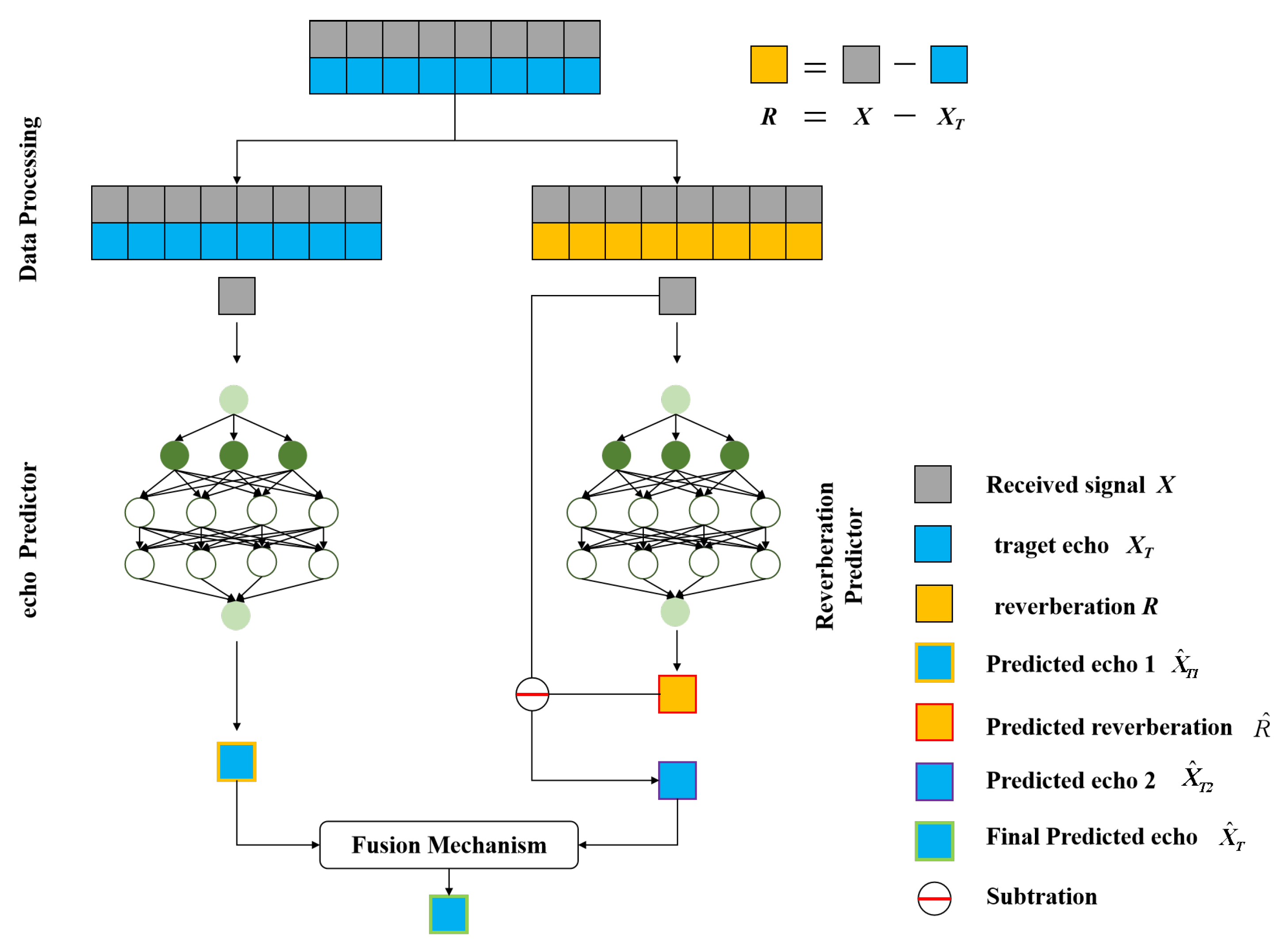
  • We proposed an ERCL strategy, which simultaneously learns the target echo and reverberation through two complementary predictors. The final target echo is reconstructed using the features extracted by these two predictors, thereby improving the model’s dereverberation performance. This strategy enables better recovery of the target echo in complex environments and reduces reverberation interference.
  • We propose a wavelet transform-based attention feature extraction method that replaces the traditional STFT with CWT. It balances time–frequency resolution and better handles the non-stationary nature of reverberation. Instead of recovering the magnitude and phase spectra, we focus on recovering the real and imaginary parts, simplifying the phase recovery process. Additionally, introducing an attention mechanism helps the network to focus on important regions of the time–frequency spectrogram, especially in complex reverberation environments.

2. Materials and Methods
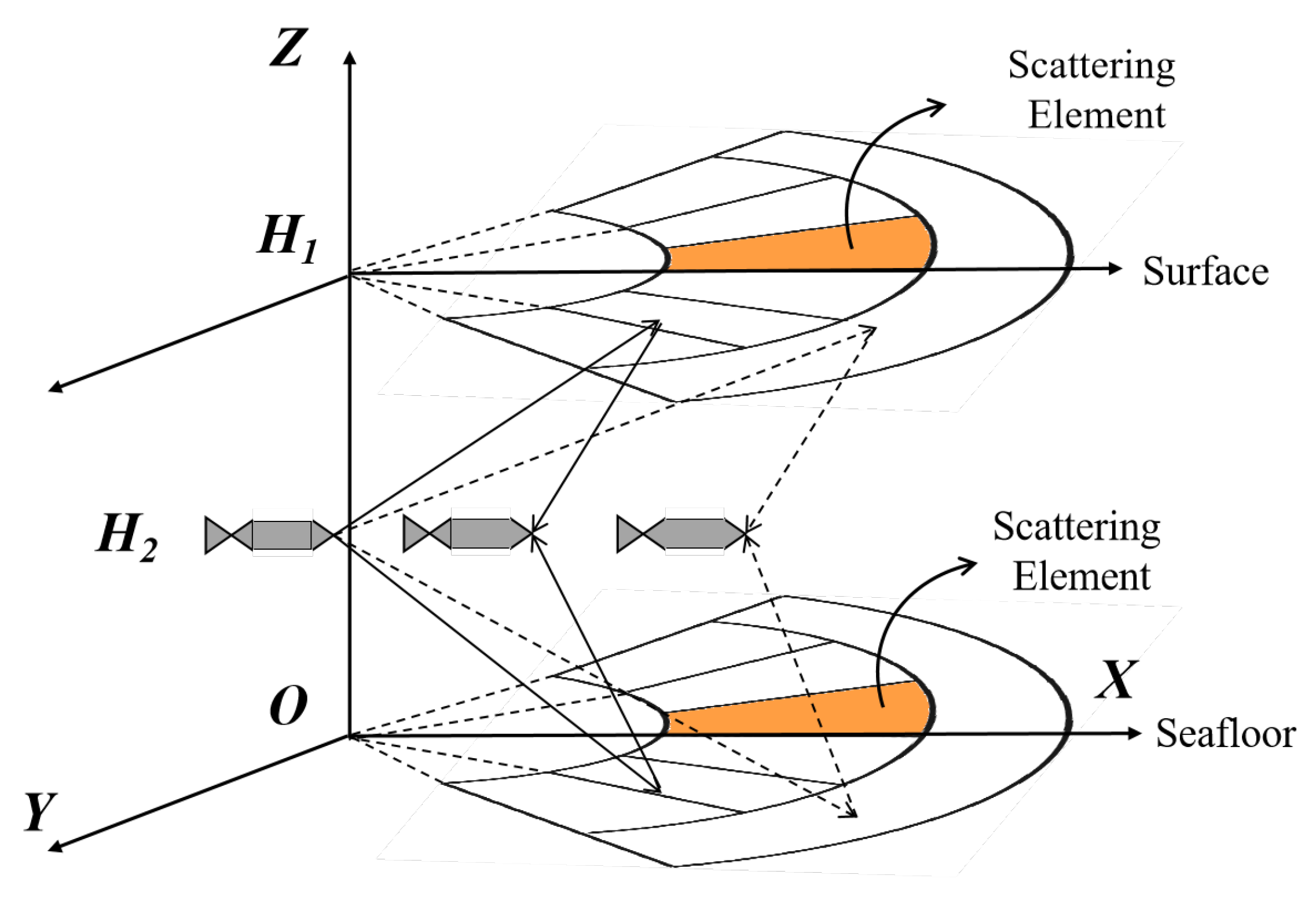
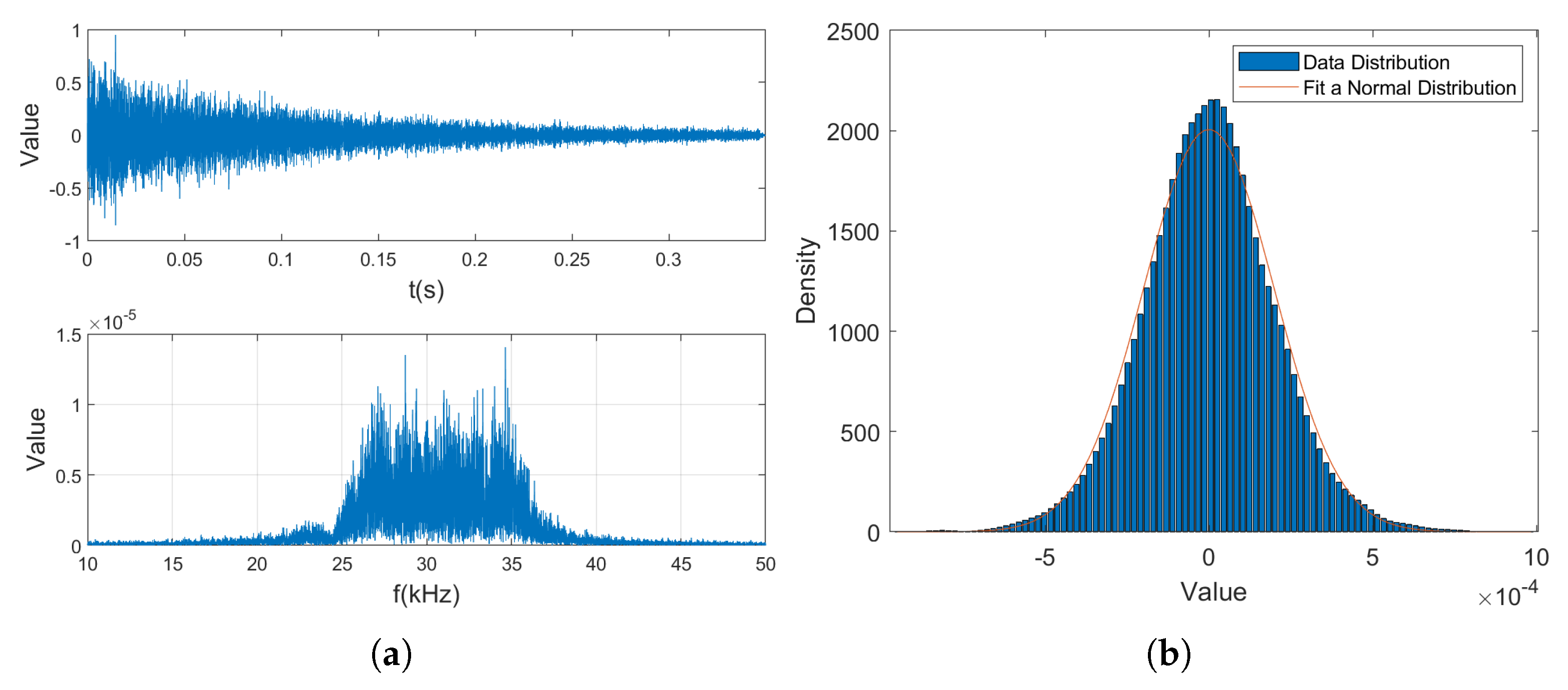
2.1. Data Modeling

Figure 1 displays the framework of received signal modeling. It outlines the acoustic propagation from the transmission to the observed output. The model accounts for the signal’s interaction with the ocean channel and target scattering. It incorporates the Doppler Effect (DE) and the Signal-to-Reverberation Ratio (SRR) adjustment to generate the observed signal.
Assume the transmitted broadband signal is denoted by s ( t ) . The interaction of the acoustic signal with the channel and the target primarily influences the signal’s amplitude, phase, delay, and Doppler effect. Initially focusing on the delay and the Doppler effect, the received signal at a single array element due to a single highlight can be expressed as
s r ( t ) = s ( ( 1 + a ) ( t τ ) )
where a represents the Doppler stretching factor, defined as
a = 2 v c
Here, v is the radial velocity between the target and the sonar, c is the speed of sound, and τ is the time delay [43].
Applying a discrete Fourier transform to s r ( t ) , the broadband is segmented into Q narrowbands, yielding the frequency domain data S r ( f ) . Considering the amplitude and phase variations introduced by the interaction of the acoustic signal with the target and the channel, and taking into account the wave direction θ , the received signal by an M-element uniform linear array, with element spacing d, can be represented as
X ( f q ) = b e j φ q a ( f q , θ ) S r ( f q )
where a ( f q , θ ) is the steering vector, given by
a ( f q , θ ) = 1 , exp j 2 π f q d cos ( θ ) c , , exp j 2 π f q ( M 1 ) d cos ( θ ) c T
In this expression, b is the amplitude factor affected by propagation loss and target scattering, and φ q is the phase shift at frequency f q .
As shown in Figure 2, a finite element scattering model is employed to model the reverberation, treating reverberation as a superposition of scattered echoes excited by scattering units at the receiving end [44]. The main steps involved in reverberation simulation include the division of scattering cells, the calculation of scattering parameters, and the formation of the array-received signal. First, the receiver’s receiving sector is divided into small scattering cells based on distance and azimuth. Next, parameters such as scattering intensity, propagation loss, time delay, and Doppler factor are calculated for each scattering unit. Each scattering unit is then treated as a tiny target to generate the echo signals received by the array. Finally, the reverberation signals from all scattering units are superimposed to obtain the total reverberation.
Following the above process, the reverberation received by the array can be expressed as
R ( f q ) = i = 1 N 1 K i · S i f q e j ϕ i q a T ( θ i , f q )
where N 1 represents the number of scatterers contributing to the reverberation at time t. K i represents the amplitude factor affected by channel propagation loss, namely interface scattering. It can be calculated by the following formula:
K i = 10 E L i 20
E L i = S L 2 T L i + S s i
where S L denotes the source level of the transmitted signal; T L i is the one-way transmission loss for the i-th scatterer; The backscattering strength of the i-th scatterer, denoted as S s i , is governed by different models depending on the scattering environment: for the sea bottom, it follows Lambert’s law; for the sea surface, it is described by the empirical formula of Chapman and Harris; and for the volume, it is modeled using the Love model [45]. In addition, the part of K i influenced by scattering includes Gaussian random disturbances with a mean of 0. ϕ i q is the random phase, which follows a uniform distribution in the range (0,2 π ) and a ( θ i , f q ) is the array steering at the i-th scatterer and q-th frequency point.
The time-domain signal X T ( t ) and R ( t ) can be recovered by applying an inverse Fourier transform to Equations (3) and (5). Thus, the array received signal for active sonar can be expressed as
X ( t ) = X T ( t ) + R ( t )

2.2. Preprocessing

The CWT offers significant advantages over the STFT in time–frequency analysis. The STFT uses a fixed window function for local Fourier transforms, resulting in poor time–frequency resolution for low-frequency signals and inadequate frequency resolution for high-frequency signals. Compared with it, the CWT adaptively adjusts the scale and position of the wavelet basis. It avoids the resolution trade-off inherent in the STFT [46]. As a result, the CWT is better suited to tracking instantaneous frequency changes in signals, particularly non-stationary signals. The CWT demonstrates enhanced adaptability and accuracy when processing non-stationary signals, such as reverberation. Therefore, in this paper, we choose the CWT to extract the time–frequency features of the signal.
The mathematical expression for CWT is
CWT ( x ( t ) , ψ , b ) = x ( t ) ψ * t b a d t
where x ( t ) is the input signal and ψ ( t ) is the wavelet function. a is the scale factor that controls the frequency resolution of the wavelet. b is the translation factor, representing the translation of the wavelet along the time axis. ψ * ( t ) is the complex conjugate of the wavelet function.
When the CWT utilizes a complex wavelet basis, it typically outputs a complex result. The amplitude spectrogram represents the signal’s energy, while the phase spectrogram captures how the frequencies are combined. The phase spectrogram plays a crucial role in signal recovery, directly impacting the recovered time-domain waveform. However, under low signal-to-reverberation ratios (SRRs), recovering the phase spectrogram becomes complicated due to interference. Therefore, in this paper, the real and imaginary parts of the CWT results are extracted and concatenated to serve as input for the subsequent network. This approach avoids the difficulty of directly recovering the phase spectrogram while retaining sufficient time–frequency information, thereby improving recovery accuracy.
In this task, the deep learning model performs dereverberation on the time–frequency spectrogram, removing reverberation components by learning the features of both the target echo and reverberation. The dereverberated time–frequency spectrogram serves as the model’s output. This processed spectrogram is then recovered into the acoustic signal via the inverse Continuous Wavelet Transform (ICWT), as given by the following formula:
x ( t ) = 1 C ψ W ( a , b ) ψ t b a d a a 2
where C ψ is a constant dependent on the choice of wavelet function and W ( a , b ) is the time–frequency domain representation obtained by CWT.
At this stage, the end-to-end dereverberation task is complete.

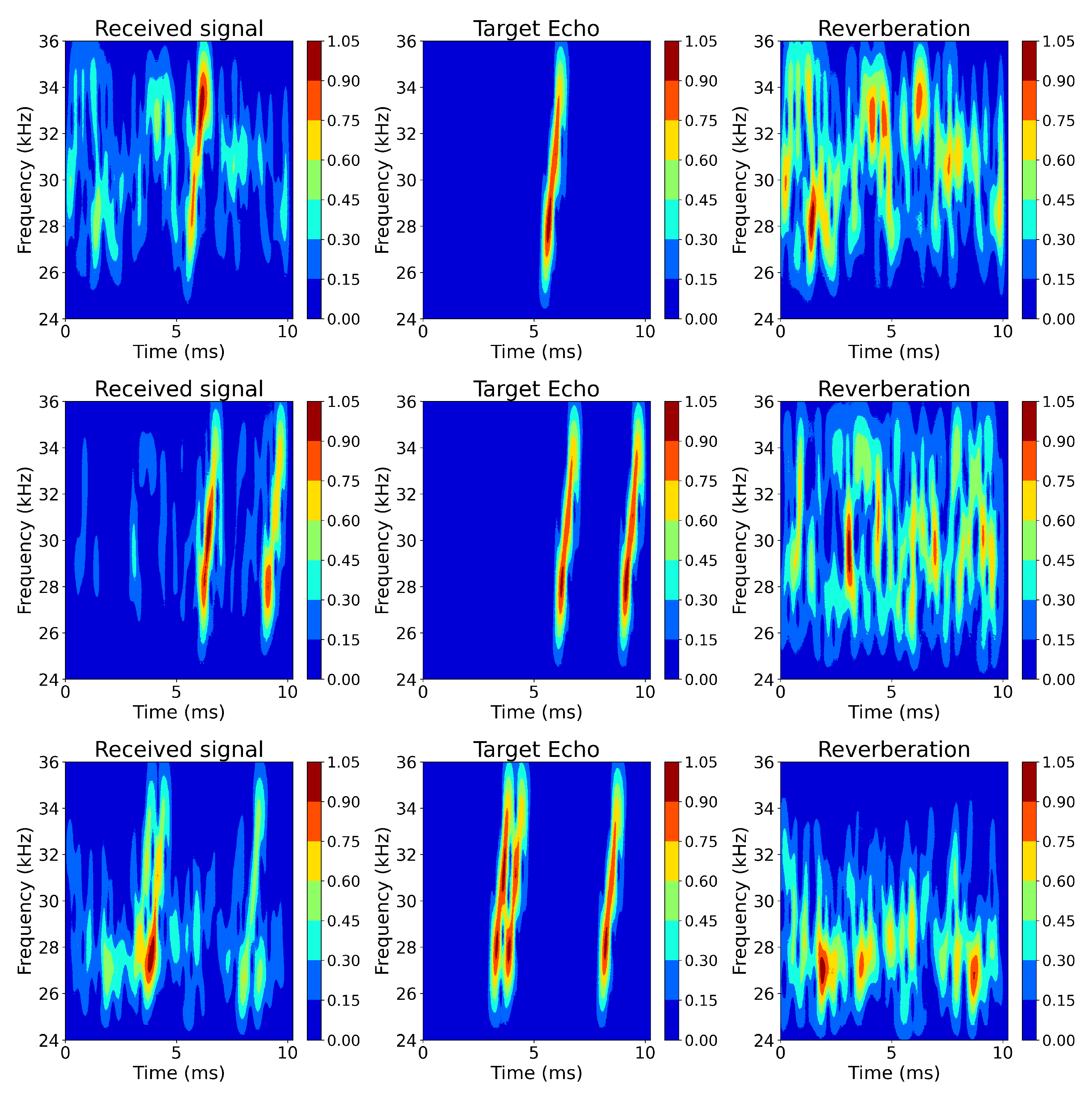
2.3. Echo–Reverberation Complementary Learning Strategies

Assume that X is the received signal in the beamforming domain, which is affected by reverberation. It is the superposition of the target echo X T and the reverberation R.
X = X T + R
Existing deep-learning-based dereverberation methods can be divided into two categories. One category is the spectral mapping method, which directly maps the received signal to the target echo:
X ^ T 1 = p e ( X )
where X ^ T 1 denotes the predicted target echo, and P e is the target echo predictor.
The other category is the residual mapping method, where reverberation is first predicted, and the final target echo is obtained by subtracting the predicted reverberation from the input received signal:
X ^ T 2 = X R ^ = X p r ( X )
where R ^ denotes the predicted reverberation and P r is the reverberation predictor.
Spectral mapping and residual mapping each have their advantages: Spectral mapping can fully leverage the spectral characteristics of the target signal, suppress reverberation, and preserve the intrinsic features of the target echo in clearer scenarios, making it especially suitable for cases with a high SRR. On the other hand, residual mapping handles complex reverberation scenarios more effectively, especially when the SRR is relatively low. In such cases, the network can focus more on removing the reverberation component while retaining key information from the target echo, thereby improving the robustness and adaptability of the dereverberation process. To combine the advantages of both approaches, we propose an ERCL strategy, as shown in Figure 3, where both spectral mapping and residual mapping are used complementarily. ERCL treats dereverberation as an end-to-end task, where the input is the received signal X, and the output is the predicted target echo X ^ T . The entire ERCL dereverberation process can be expressed by the deep learning function F as follows:
X ^ T = F ( X ) = f ( X ^ T 1 , X ^ T 2 ) = f ( p e ( X ) , X p r ( X ) )
Here, X ^ T 1 is the output of the echo predictor P e , R ^ is the output of the reverberation predictor P r , X ^ T 2 is the difference between the received signal X and the predicted reverberation R ^ , and f denotes the fusion mechanism. Firstly, X is used as the input to P e and P r to obtain the predicted target echo X ^ T 1 and the predicted reverberation R ^ , respectively. Then, by subtracting R ^ from the received signal X, another predicted target echo X ^ T 2 is computed. Finally, through the fusion mechanism f, X ^ T 1 and X ^ T 2 are combined to obtain the final predicted target echo X ^ T .
The learning process of ERCL can be framed as an optimization problem:
arg min F F ( X ) X T 2 2
In this work, we propose a dereverberation process based on the ERCL strategy for a given signal pair { X , X T } . The reverberation component R is computed using the relation X = X T + R , forming two signal pairs: { X , X T } and { X , R } . The pair { X , X T } is used to train the model P e , while the pair { X , R } is used to train the model P r .

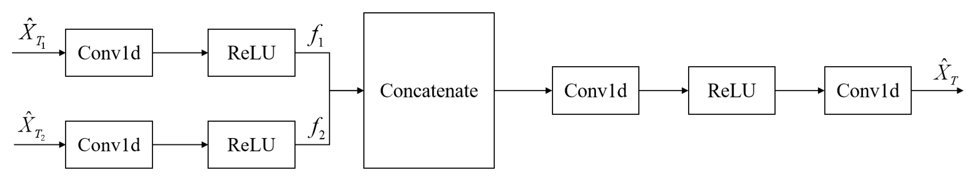
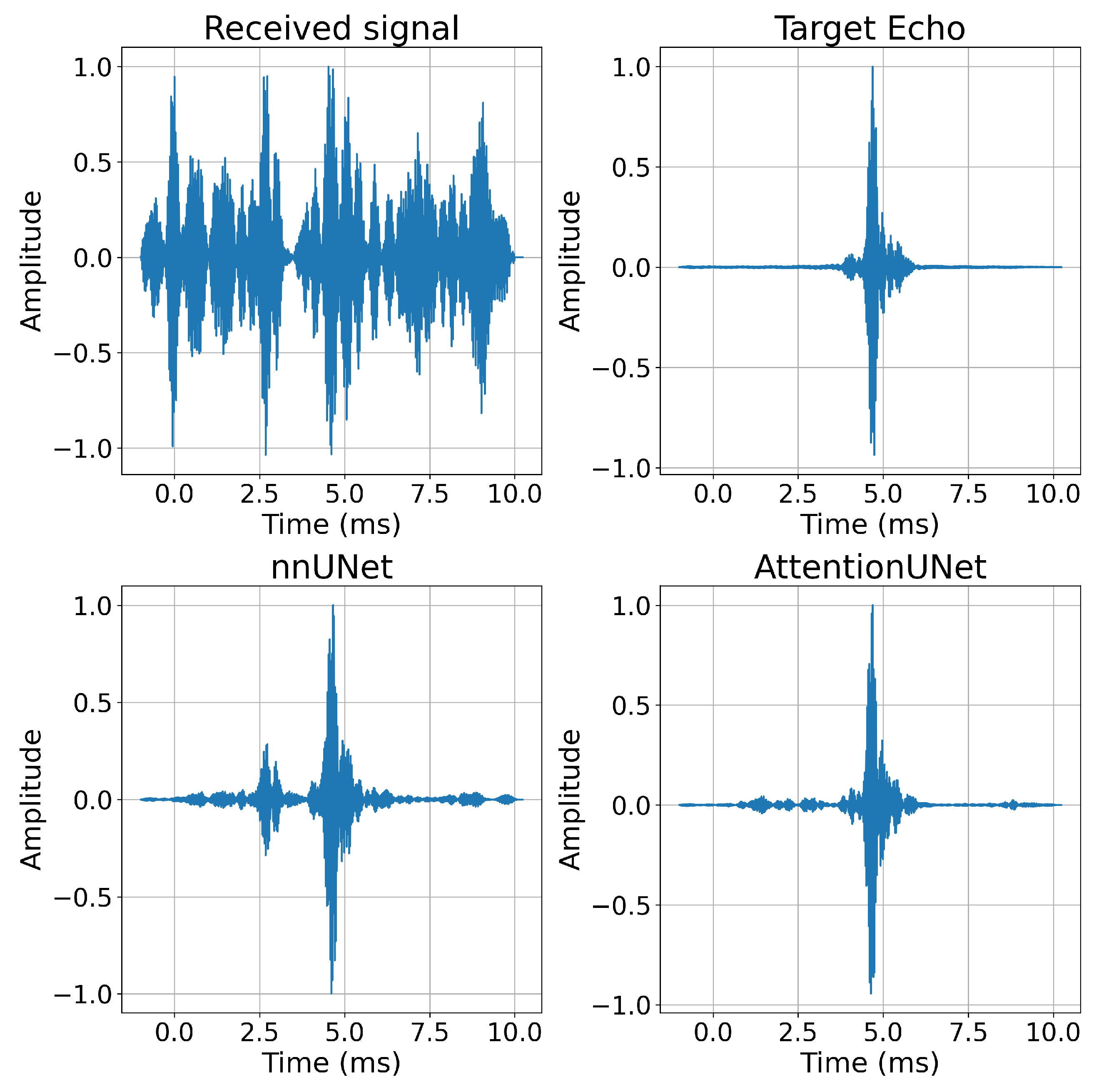
2.4. ERCL-AttentionNet

2.4.1. Overall Architecture

In this study, we propose a novel network architecture, ERCL-AttentionNet, for the dereverberation task of active sonar, as shown in Figure 4. The network consists of an encoder, two decoders, and a fusion mechanism.
The encoder is a key component responsible for extracting features from the input signal. It consists of several processing stages, comprising two structured convolutional blocks and a max-pooling layer. Each convolutional block consists of a 3 × 3 convolutional layer, a batch normalization (BN) layer, and a ReLU activation function arranged in sequence. This combination of layers enhances the model’s feature extraction capabilities and helps prevent overfitting. After each convolutional block, a 2 × 2 max-pooling operation is applied, performing spatial downsampling of the feature map while doubling the number of feature channels, thereby providing a higher-resolution feature representation. Additionally, the encoder includes skip connections that directly pass the feature maps from each layer to the corresponding layer in the decoder. This helps preserve crucial spatial information during the subsequent decoding process.
The decoder section comprises two parallel decoders. They share a similar architecture but are responsible for recovering the CWT spectrograms of the target echo and reverberation. Each decoder contains a 2 × 2 deconvolution operation for up-sampling. This operation improves the spatial resolution of the feature maps while reducing the number of feature channels by half. The up-sampled feature maps are concatenated with the corresponding feature maps from the encoder via skip connections. An attention mechanism is applied to assign weights to the concatenated feature maps during this process. It helps the network focus on the most relevant regions, improving the recovery of the target echo and reverberation. The concatenated feature maps are further processed through structured convolutional blocks. This design enables the decoders to progressively recover detailed information about the target echo and reverberation. Finally, the CWT spectrograms output by both decoders are transformed back into 1D speech signals. This is accomplished using the ICWT, which forms the basis for subsequent fusion steps.
The fusion mechanism shown in Figure 5 is based on the ERCL strategy, which first obtains independent estimates of the target echo and reverberation from the two decoders. These estimates are then fused into a single output. The essence of the method is focused on extracting local features from the input signals via convolutional operations and performing fusion at the feature level to enhance the signals and achieve information complementarity. Specifically, we first use independent one-dimensional convolutional layers to extract features from the two input signals. The extracted features are then concatenated along the channel dimension and integrated using a fusion convolutional layer to capture their interaction. Finally, the fused features are mapped back to the signal space using a reconstruction convolutional layer, producing the fused target echo.

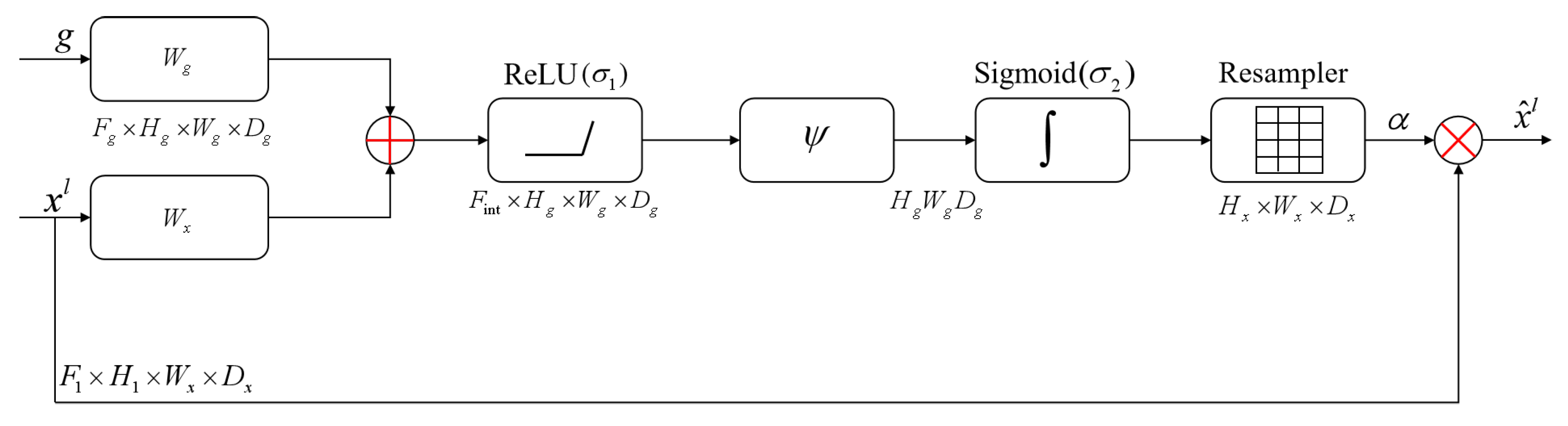
2.4.2. Attention Gate

The Attention Gate, as shown in Figure 6, takes two inputs: the feature map from the decoder G, which serves as the gating signal, and the feature map from the encoder X , which is to be weighted. In order to align perfectly with the dimensions of the encoder feature map, the decoder feature map is up-sampled. Next, two convolutional layers, W g and W x , are applied to learn the weights for the gating signal and the encoder feature map. These are then summed, with nonlinearity introduced via the ReLU activation function. Finally, a 1 × 1 convolution followed by a Sigmoid activation function generates the attention coefficients, which enhance the encoder feature map.

2.4.3. Loss Function

Since the proposed ERCL-AttentionNet combines target echo features with reverberation features, the loss function is defined as the mixing loss:
L = L T + λ 1 L R + λ 2 L F
where L T , L R , and L F represent the losses for the target echo prediction, reverberation prediction, and the final fusion process, respectively. λ 1 and λ 2 are the weighting factors that balance the recovery of the target echo and the reverberation.
For residual mapping, we first recover the residual component of the target echo by predicting the reverberation in the time–frequency domain. Let the spectrogram of the reverberation be denoted as S R and the spectrogram of the predicted reverberation be S ^ R ; then, the reverberation learning loss L R can be expressed as
L R = S R S ^ R 2 2
where · 2 2 denotes the conventional L 2 norm, representing the difference between the spectrogram of the predicted reverberation and the true reverberation.
Spectral mapping aims to recover the target echo from the reverberant signal. Assume that the predicted spectrogram of the target echo is S ^ T and the actual spectrogram of the target echo is S T ; then, the target echo learning loss L T can be expressed as
L T = S T S ^ T 2 2
The ultimate objective is to fuse residual mapping and spectral mapping to recover a pure acoustic signal, which requires combining the losses from both mapping types to optimize the final output. Assume that the final recovered 1D acoustic signal is X ^ T , and the true target echo is X T ; then, this part of the loss can be expressed as
L F = X T X ^ T 2 2

3. Dataset Construction and Experimental Setup

3.1. Dataset Construction

Due to the absence of publicly available datasets in the field of active sonar, this paper constructs a dataset consisting of 14,580 samples generated using the finite element scattering model and the highlight model. Each sample contains 1024 sampling points, which are processed using the CWT and converted into a time–frequency spectrogram with dimensions of 2 × 512 × 1024 for model training and testing. The details of the dataset simulation are provided in Table 1.
The simulation parameters are as follows: the source level of the sonar transducer is 220 dB, the underwater speed of sound is 1500 m/s, the emission period is 1.5 s, and the sonar platform moves at a constant speed of 50 knots at a depth of 30 m below the sea surface. The ocean channel depth is 60 m, and the distance from the target to the seafloor is 30 m. The array consists of 52 elements, arranged horizontally and vertically as 4, 6, 8, 8, 8, 8, 6, 4, with half-wavelength spacing between the array elements. The sonar detection range spans from −45° to 45° in horizontal azimuth and from −10° to 10° in pitch.
In the simulation, nine LFM signals are used as the transmitted signals. These signals consist of a combination of a center frequency of 30 kHz, three pulse widths (1 ms, 2 ms, and 3 ms), and three bandwidths (6 kHz, 8 kHz, and 10 kHz). The simulation generates three underwater targets with one, two, or three highlight point structures. Nine LFM signals are applied to these three targets, generating 27 target echoes. The targets are simulated at 60 different angular positions within the sonar detection range, with each angle having a distinct scenario to enhance data diversity, modeling various potential sonar-target spatial scenarios. As a result, the relative time delay, relative intensity, and phase jump of the corresponding highlight echoes in Equation (3) for each target vary. The simulation of reverberation is based on the finite element scattering model shown in Figure 2. According to Equation (5), random variations are added to the scattering coefficients and phases of each scatterer during the simulation. Since the position of the target echo is arbitrary, a random truncation method is used when mixing the reverberation and target echoes.
Finally, to study the reverberation suppression performance under different SRRs, nine SRRs are used to reconstruct the array-received signals. Beamforming is then performed at the target location, resulting in 14,580 observed signals, which are used as the network’s dataset. The dataset is divided into a training set, validation set, and test set at a ratio of 8:1:1.
Figure 7 presents the time-domain waveform, spectrum, and probability density distributions of the instantaneous values, mode values, and phases of the reverberation data for a transmitted signal with a bandwidth of 25 kHz to 35 kHz and a pulse width of 3 ms. These results are compared to theoretical values. The theoretical analysis suggests that the instantaneous value of the reverberation follows a Gaussian distribution, the envelope follows a Rayleigh distribution, and the phase follows a uniform distribution. The simulation data closely matches the theoretical predictions [47,48], providing reliable experimental data to support subsequent research.
Figure 8 illustrates a portion of the dataset, displaying the time–frequency spectrograms of the received signal, target echo, and reverberation from left to right. The time–frequency spectrogram of the received signal captures the combined characteristics of the target echo and reverberation, resulting in a more complex time–frequency distribution. The time–frequency spectrogram of the target echo exhibits a more focused frequency distribution. The spectrogram of the reverberation displays more complex time–frequency characteristics, such as significant fluctuations and extensions.

3.2. Experimental Setup

The datasets are constructed using MATLAB R2022b. The preprocessing process and the reverberation suppression network are developed using PyTorch 2.0.0 and Python 3.9. Training is conducted on an Nvidia GeForce GTX 3090 GPU with Nvidia CUDA 12.6. During training, the network’s initial learning rate is set to 2 × 10 3 , with parameters updated through adaptive learning rate adjustments using the Adam optimizer. The batch size for the input data is set to 8, and the network is trained for 50 iterations.

4. Results

4.1. Evaluation Metrics

We use the Peak-to-Average Signal-to-Reverberation Ratio (PSRR), the Structural Similarity Index (SSIM), and the Peak-to-Average Power Ratio (PAPR) of Cross-Correlation as evaluation metrics for dereverberation performance.

4.1.1. PSRR

PSRR is a performance evaluation metric based on the Mean Square Error (MSE), which measures the error between the reconstructed signal spectrogram and the target echo spectrogram. The formula calculates PSRR:
PSRR = 10 log 10 MAX 2 MSE
where MAX is the maximum value of the spectrogram and MSE is the mean square error, denoted as
MSE = 1 N i = 1 N x ( i ) y ( i ) 2
x ( i ) and y ( i ) are the spectrograms of the target echo and the reconstructed signal, respectively, at the i-th amplitude at the position.
PSRR can effectively quantify the error between the reconstructed signal and the spectrogram of the target echo. A higher PSRR value usually indicates a minor error between the reconstructed signal and the target echo, thus reflecting a better dereverberation performance.

4.1.2. SSIM

SSIM measures the similarity between signals by comparing their spectrograms’ brightness, contrast, and structural information. SSIM is calculated using the following formula:
SSIM ( x , y ) = ( 2 μ x μ y + C 1 ) ( 2 σ x y + C 2 ) ( μ x 2 + μ y 2 + C 1 ) ( σ x 2 + σ y 2 + C 2 )
where x and y represent the spectrograms of the target echo and the reconstructed signal, respectively. μ x and μ y denote the mean values of the signal spectrograms. σ x and σ y represent their standard deviations. C 1 and C 2 are constants added to avoid division by zero. A higher SSIM value indicates fewer errors between the reconstructed and original signals. A SSIM of 1 means the signals are identical, showing optimal dereverberation performance.

4.1.3. PAR

The Peak-to-Average Ratio (PAR) of cross-correlation is an important metric for evaluating the performance of signal processing in radar and sonar systems. It is achieved by calculating the cross-correlation function between the received signal x and the replica of the transmitted signal y and then analyzing the ratio of the peak to the average power of this function. The formula for calculating the PAR of cross-correlation is as follows:
PAR = max ( R x y ) R x y ¯
where R x y represents the cross-correlation function between the received signal x and the the transmitted signal y. R x y ¯ represents the mean value of R x y . The PAR of cross-correlation reflects the detectability of the target echo against the background noise and interference. A higher PAR of cross-correlation implies a higher degree of matching between the target echo and the transmitted signal, making it easier to detect amid noise.

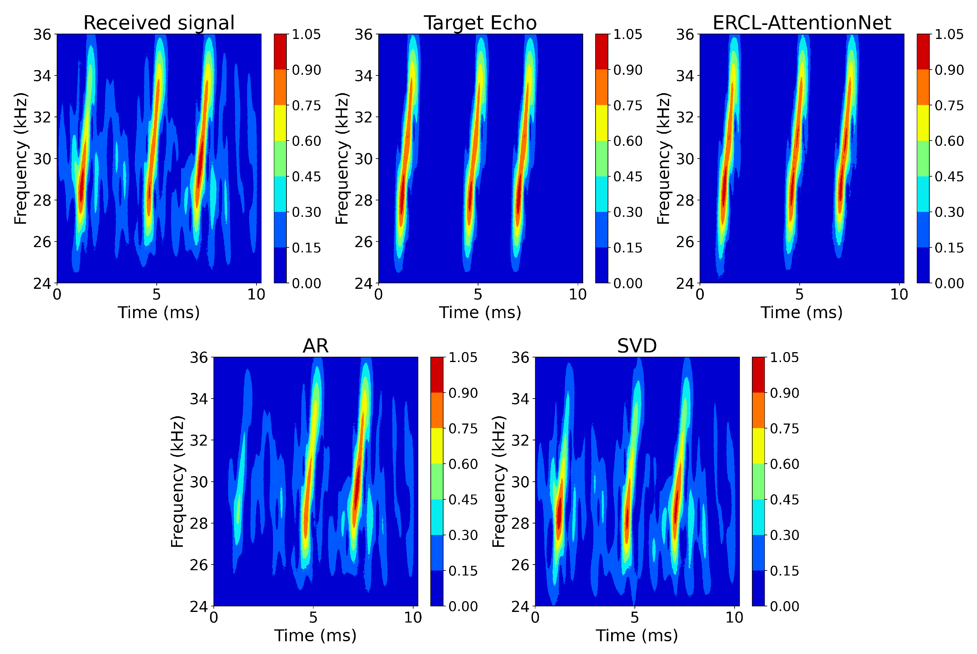
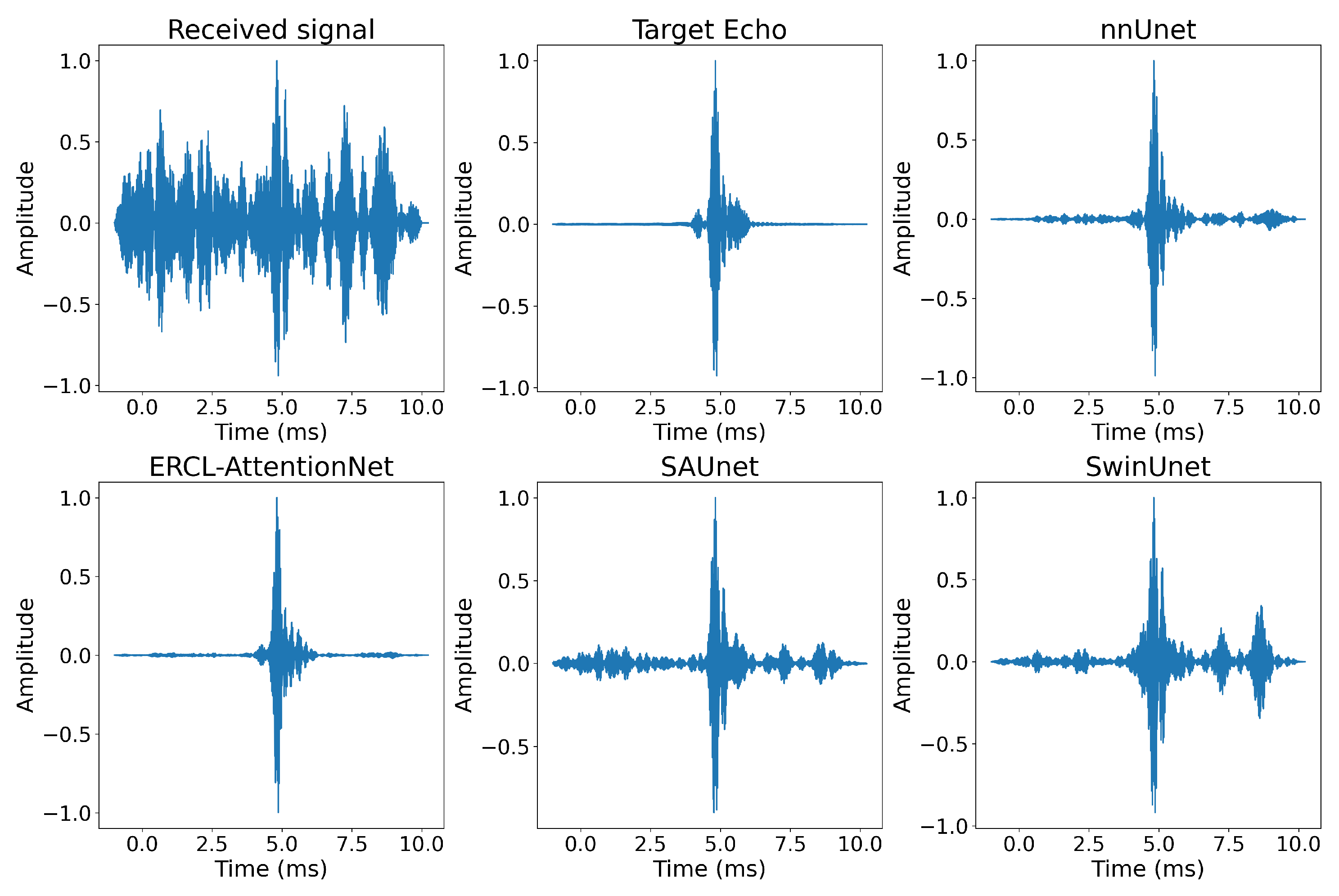
4.2. Evaluation Results

Firstly, we conduct ablation experiments to evaluate the effectiveness of each model component. We also explore the impact of introducing the attention mechanism and complementary learning strategy on dereverberation performance. Table 2 lists the key metrics of each model, including PSRR, SSIM, and PAR. Figure 9 shows the dereverberation results before and after introducing the attention mechanism. Figure 10 shows the output results of dereverberation after incorporating the complementary learning strategy.
As shown in Figure 9, introducing the attention mechanism helps the model concentrate on the target area, making the recovered spectrogram more concentrated. The reverberation within the red box is further suppressed. Following Figure 9, Figure 10 shows the cross-correlation results between the model outputs and the transmitted signal, further demonstrating the enhanced performance of the AttentionUNet model in reverberation suppression. The traditional UNet model for target echo recovery has a PSRR of 31.681 dB, a SSIM of 0.864, and a PAR of 27.035. In comparison, the AttentionUNet model improves PSRR by approximately 2.09 dB, increases SSIM by around 0.06, and improves PAR by about 2.95, highlighting the effectiveness of the attention mechanism in enhancing reverberation suppression.
Figure 11 shows that the complementary learning strategy helps the model distinguish between reverberation and non-reverberation. The area within the red box is reverberated; the ERCL strategy corrects this in the reverberation predictor. Figure 12 presents the cross-correlation results, where the ERCL strategy significantly suppresses reverberation around 2 s and enhances the target echo. Compared to the AttentionUNet model, the ERCL strategy improves PSRR by 0.6 dB, SSIM by 0.02, and PAR by 1.036, demonstrating its effectiveness in enhancing dereverberation quality. These results confirm that both the attention mechanism and the complementary learning strategy improve dereverberation performance.
Then, we conducted a comparative experiment to evaluate the performance of our method against traditional dereverberation methods. The AR model (p = 2) and binary SVD were selected as baseline methods. Figure 13 and Table 3 show the differences in recovery quality across different methods.
Figure 13 shows that the AR method and binary SVD could only remove part of the reverberation and failed to suppress it effectively. As a result, the recovery of target signal details was poor. In scenarios with multiple bright structures and more complex time–frequency plots, reverberation remained prominent, and the recovered target signal showed distortion and loss of details. In contrast, ERCL-AttentionNet successfully removed the reverberation, achieving a PSRR of 35.208 dB and a SSIM of 0.948, significantly higher than the AR and SVD methods.
Figure 13 shows that the AR method and binary SVD could only partially remove the reverberation, failing to suppress it effectively. Figure 14 presents the cross-correlation results between the model outputs and the transmitted signal. Compared to AR and SVD, ERCL-AttentionNet demonstrated more pronounced peaks at three locations in the cross-correlation results, effectively removing the reverberation. ERCL-AttentionNet achieved a PSRR of 35.208 dB, a SSIM of 0.948, and a PAR of 31.018, all significantly higher than those of the AR and SVD methods, further confirming its superior performance.
Finally, we compared the performance of various dereverberation models, including nnUNet, AttentionUNet, SAUNet, SwinUNet, and ERCL-AttentionNet. The results are shown in Table 4, Figure 15 (CWT spectrogram), and Figure 16 (cross-correlation between model outputs and transmitted signal).
The experimental results indicate that nnUNet performs relatively poorly in the dereverberation task, with a PSRR of 31.681 dB, a SSIM of 0.864, and a PAR of 27.035. The method does not suppress reverberation effectively. In contrast, after incorporating the attention mechanism, Attention U-Net shows significant improvement in dereverberation, with a PSRR increase of 2.902 dB, a SSIM improvement of 0.061, and a PAR increase of 2.947. This enhancement indicates a marked improvement in dereverberation quality. SAUNet performs poorly in the dereverberation task, with a PSRR of 27.568 dB, SSIM of 0.654, and PAR of 23.025. This is mainly due to its difficulty balancing computation load and performance, which results in ineffective suppression of reverberation and poor recovery of the target signal. The performance of SwinUNet is also limited, with a PSRR of 29.756 dB, SSIM of 0.803, and PAR of 26.014. This limitation is due to its high input spectrogram and window size requirements, making it challenging to find the optimal parameters for the best recovery, and the reverberation components were not entirely removed.
Ultimately, ERCL-AttentionNet outperforms all other models. It combines the attention mechanism with the complementary learning strategy, significantly improving recovery quality. The model not only effectively suppresses reverberation but also preserves the details of the target signal, demonstrating stronger robustness and recovery capability.

5. Conclusions

In this paper, we construct an active sonar dataset based on the finite element scattering and highlight models. It effectively addresses the gap in available underwater datasets. The amplitude of simulated reverberation follows a Gaussian distribution, the mode value follows a Rayleigh distribution, and the phase follows a uniform distribution, aligning with the theoretical expectations. It validates the reliability of the dataset.
Building upon this, we propose a network model, ERCL-AttentionNet, which integrates the reverberation echo complementary learning method with the attention-guided wavelet transform. The model extracts time–frequency features from the received signal using Continuous Wavelet Transform and learns the target echo and reverberation features simultaneously through two complementary predictors, enabling the reconstruction of the target signal. Experimental results demonstrate that ERCL-AttentionNet outperforms other methods in both qualitative and quantitative evaluations. Compared to traditional AR and SVD methods, our approach effectively removes reverberant interference while preserving the time–frequency structural characteristics of the target echo, achieving a PSRR of 35.208 dB, a SSIM of 0.948, and a PAR of 31.018.
In conclusion, the ERCL strategy proposed in this paper demonstrates substantial effectiveness in active sonar dereverberation tasks and shows promising potential for practical engineering applications.

Author Contributions

Conceptualization, J.L., Z.P. and X.C.; Methodology, J.L. and Z.P.; Software, J.L.; Writing—Original Draft Preparation, J.L. and C.T.; Writing—Review and Editing, J.L., Q.Z., X.C. and C.T.; Funding Acquisition, Q.Z. All authors have read and agreed to the published version of the manuscript.

Funding

This research was funded by the National Natural Science Foundation of China, grant number 62371393, from January 2024 to December 2027.

Institutional Review Board Statement

Not applicable.

Informed Consent Statement

Not applicable.

Data Availability Statement

The data presented in this study are available on request from the corresponding author due to privacy.

Conflicts of Interest

The authors declare no conflicts of interest.

References

  1. Zhou, X.; Wang, N.; Yan, Y.; Yang, K. Underwater detection of small-volume weak target echo in harbor scene under multisource interference. IEEE Geosci. Remote Sens. Lett. 2022, 19, 1–5. [Google Scholar] [CrossRef]
  2. Chu, N.; Ning, Y.; Yu, L.; Liu, Q.; Huang, Q.; Wu, D.; Hou, P. Acoustic source localization in a reverberant environment based on sound field morphological component analysis and alternating direction method of multipliers. IEEE Trans. Instrum. Meas. 2021, 70, 1–13. [Google Scholar] [CrossRef]
  3. Trucco, A. Experimental results on the detection of embedded objects by a prewhitening filter. IEEE J. Ocean. Eng. 2001, 26, 783–794. [Google Scholar] [CrossRef]
  4. Kay, S.; Salisbury, J. Improved active sonar detection using autoregressive prewhiteners. J. Acoust. Soc. Am. 1990, 87, 1603–1611. [Google Scholar] [CrossRef]
  5. Jiang, L.; Pan, Y.; Tang, J. Multi-Level Binary SVD for Sonar Reverberation Suppression. In Proceedings of the 2018 OCEANS-MTS/IEEE Kobe Techno-Oceans (OTO), Kobe, Japan, 28–31 May 2018; pp. 1–4. [Google Scholar]
  6. Wang, M.; Wu, S.; Guo, S.; Peng, D. Study on an anti-reverberation method based on PCI-SVM. Appl. Acoust. 2021, 182, 108189. [Google Scholar] [CrossRef]
  7. Li, P.; Qiu, H.A.; Wang, C.; Wu, Y.; Miao, F. Research on reverberation cancellation algorithm based on empirical mode decomposition. In Proceedings of the 2020 IEEE International Conference on Information Technology, Big Data and Artificial Intelligence (ICIBA), Chongqing, China, 6–8 November 2020; Volume 1, pp. 941–945. [Google Scholar]
  8. Jia, L.; Feng, X.; Juan, Y.; Xudong, A. The bottom reverberation suppression algorithm for side scan sonar. In Proceedings of the 2014 Oceans-St. John’s, St. John’s, NL, Canada, 14–19 September 2014; pp. 1–4. [Google Scholar]
  9. Yuan, F.; Xiao, F.; Zhang, K.; Huang, Y.; Cheng, E. Noise reduction for sonar images by statistical analysis and fields of experts. J. Vis. Commun. Image Represent. 2021, 74, 102995. [Google Scholar] [CrossRef]
  10. Khan, D.M.; Yahya, N.; Kamel, N. Optimum order selection criterion for autoregressive models of bandlimited EEG signals. In Proceedings of the 2020 IEEE-EMBS Conference on Biomedical Engineering and Sciences (IECBES), Langkawi Island, Malaysia, 1–3 March 2021; pp. 389–394. [Google Scholar]
  11. Libal, U.; Johansson, K.H. Yule-Walker equations using higher order statistics for nonlinear autoregressive model. In Proceedings of the 2019 Signal Processing Symposium (SPSympo), Krakow, Poland, 17–19 September 2019; pp. 227–231. [Google Scholar]
  12. Cao, Y.; Zhang, Q. Spatio-Temporal Reverberation Suppression Method Based on Itakura Distance Segmental Pre-Whitening and Progressive Adaptive Binary SVD. In Proceedings of the 2024 IEEE International Conference on Signal Processing, Communications and Computing (ICSPCC), Bali, Indonesia, 19–22 August 2024; pp. 1–6. [Google Scholar]
  13. Sun, Y.; Zhou, Y.; Xu, X.; Qi, J.; Xu, F.; Ren, Z. Weakly-Supervised Depression Detection in Speech Through Self-Learning Based Label Correction. IEEE Trans. Audio Speech Lang. Process. 2025, 33, 748–758. [Google Scholar] [CrossRef]
  14. Cho, S.; Wee, K. Multi-Noise Representation Learning for Robust Speaker Recognition. IEEE Signal Process. Lett. 2025, 32, 681–685. [Google Scholar] [CrossRef]
  15. Zheng, R.C.; Ai, Y.; Ling, Z.H. Incorporating Ultrasound Tongue Images for Audio-Visual Speech Enhancement. IEEE/ACM Trans. Audio Speech Lang. Process. 2024, 32, 1430–1444. [Google Scholar] [CrossRef]
  16. Xu, X. Improving monaural speech enhancement by mapping to fixed simulation space with knowledge distillation. IEEE Signal Process. Lett. 2024, 31, 386–390. [Google Scholar] [CrossRef]
  17. Stoller, D.; Ewert, S.; Dixon, S.W.U. Wave-U-Net: A Multi-Scale Neural Network for End-to-End Audio Source Separation. arXiv 2018, arXiv:1806.03185. [Google Scholar]
  18. Luo, Y.; Mesgarani, N. Conv-tasnet: Surpassing ideal time–frequency magnitude masking for speech separation. IEEE/ACM Trans. Audio Speech Lang. Process. 2019, 27, 1256–1266. [Google Scholar] [CrossRef] [PubMed]
  19. Wang, K.; He, B.; Zhu, W.P. Caunet: Context-aware u-net for speech enhancement in time domain. In Proceedings of the 2021 IEEE International Symposium on Circuits and Systems (ISCAS), Daegu, Republic of Korea, 22–28 May 2021; pp. 1–5. [Google Scholar]
  20. Wang, X.; Zeng, K.; Li, G.; Xie, X.; Wang, Z. Sonar Dereverberation via Independent Component Analysis and Deep Learning. In Proceedings of the 2024 22nd IEEE Interregional NEWCAS Conference (NEWCAS), Sherbrooke, QC, Canada, 16–19 June 2024; pp. 1–5. [Google Scholar]
  21. Han, K.; Wang, Y.; Wang, D. Learning spectral mapping for speech dereverberation. In Proceedings of the 2014 IEEE International Conference on Acoustics, Speech and Signal Processing (ICASSP), Florence, Italy, 4–9 May 2014; pp. 4628–4632. [Google Scholar]
  22. Han, K.; Wang, Y.; Wang, D.; Woods, W.S.; Merks, I.; Zhang, T. Learning spectral mapping for speech dereverberation and denoising. IEEE/ACM Trans. Audio Speech Lang. Process. 2015, 23, 982–992. [Google Scholar] [CrossRef]
  23. Ernst, O.; Chazan, S.E.; Gannot, S.; Goldberger, J. Speech dereverberation using fully convolutional networks. In Proceedings of the 2018 26th European Signal Processing Conference (EUSIPCO), Rome, Italy, 3–7 September 2018; pp. 390–394. [Google Scholar]
  24. Zhao, L.; Zhu, W.; Li, S.; Luo, H.; Zhang, X.L.; Rahardja, S. Multi-resolution convolutional residual neural networks for monaural speech dereverberation. IEEE/Acm Trans. Audio Speech Lang. Process. 2024, 32, 2338–2351. [Google Scholar] [CrossRef]
  25. Santos, J.F.; Falk, T.H. Speech dereverberation with context-aware recurrent neural networks. IEEE/ACM Trans. Audio Speech Lang. Process. 2018, 26, 1236–1246. [Google Scholar] [CrossRef]
  26. Zhao, Y.; Wang, D.; Xu, B.; Zhang, T. Late reverberation suppression using recurrent neural networks with long short-term memory. In Proceedings of the 2018 IEEE International Conference on Acoustics, Speech and Signal Processing (ICASSP), Calgary, AB, Canada, 15–20 April 2018; pp. 5434–5438. [Google Scholar]
  27. Tang, X.; Du, J.; Chai, L.; Wang, Y.; Wang, Q.; Lee, C.H. A LSTM-based joint progressive learning framework for simultaneous speech dereverberation and denoising. In Proceedings of the 2019 Asia-Pacific Signal and Information Processing Association Annual Summit and Conference (APSIPA ASC), Lanzhou, China, 18–21 November 2019; pp. 274–278. [Google Scholar]
  28. Kothapally, V.; Xia, W.; Ghorbani, S.; Hansen, J.H.; Xue, W.; Huang, J. Skipconvnet: Skip convolutional neural network for speech dereverberation using optimally smoothed spectral mapping. arXiv 2020, arXiv:2007.09131. [Google Scholar]
  29. He, B.; Wang, K.; Zhu, W.P. Se-dptunet: Dual-path transformer based u-net for speech enhancement. In Proceedings of the 2022 Asia-Pacific Signal and Information Processing Association Annual Summit and Conference (APSIPA ASC), Chiang Mai, Thailand, 7–10 November 2022; pp. 696–703. [Google Scholar]
  30. Wang, Q.; Du, S.; Wang, F.; Chen, Y. Underwater target recognition method based on multi-domain active sonar echo images. In Proceedings of the 2021 IEEE International Conference on Signal Processing, Communications and Computing (ICSPCC), Xi’an, China, 17–20 August 2021; pp. 1–5. [Google Scholar]
  31. Shi, P.; He, Q.; Zhu, S.; Li, X.; Fan, X.; Xin, Y. Multi-scale fusion and efficient feature extraction for enhanced sonar image object detection. Expert Syst. Appl. 2024, 256, 124958. [Google Scholar] [CrossRef]
  32. Huang, J.H.; Wu, C.H. Memory-Efficient Multi-Step Speech Enhancement with Neural ODE. In Proceedings of the 23rd Annual Conference of the International Speech Communication Association, INTERSPEECH 2022, Incheon, Republic of Korea, 18–22 September 2022; pp. 961–965. [Google Scholar]
  33. Yu, G.; Li, A.; Zheng, C.; Guo, Y.; Wang, Y.; Wang, H. Dual-branch attention-in-attention transformer for single-channel speech enhancement. In Proceedings of the ICASSP 2022—2022 IEEE International Conference on Acoustics, Speech and Signal Processing (ICASSP), Singapore, 23–27 May 2022; pp. 7847–7851. [Google Scholar]
  34. Oppenheim, A.V.; Lim, J.S. The importance of phase in signals. Proc. IEEE 1981, 69, 529–541. [Google Scholar] [CrossRef]
  35. Cui, X.; Saif, A.; Lu, S.; Chen, L.; Chen, T.; Kingsbury, B.; Saon, G. Joint Unsupervised and Supervised Training for Automatic Speech Recognition via Bilevel Optimization. arXiv 2024, arXiv:2401.06980. [Google Scholar]
  36. Bagchi, S.; De Fréin, R. Elevato-CDR: Speech Enhancement in Large Delay and Reverberant Assisted Living Scenarios. In Proceedings of the 2024 9th International Conference on Frontiers of Signal Processing (ICFSP), Paris, France, 12–14 September 2024; pp. 153–157. [Google Scholar]
  37. Chen, P.; Nguyen, B.T.; Geng, Y.; Iwai, K.; Nishiura, T. Joint Deep Neural Network for Single-channel Speech Separation on Masking-based Training Targets. IEEE Access 2024, 12, 152036–152044. [Google Scholar] [CrossRef]
  38. da Silva, A.C.M.; Silva, D.F.; Marcacini, R.M. Artist Similarity based on Heterogeneous Graph Neural Networks. Ieee/Acm Trans. Audio Speech Lang. Process. 2024, 32, 3717–3729. [Google Scholar] [CrossRef]
  39. Kothapally, V.; Hansen, J.H. SkipConvGAN: Monaural speech dereverberation using Generative Adversarial Networks via complex time-frequency masking. IEEE/ACM Trans. Audio Speech Lang. Process. 2022, 30, 1600–1613. [Google Scholar] [CrossRef]
  40. Li, G.; Deng, J.; Geng, M.; Jin, Z.; Wang, T.; Hu, S.; Cui, M.; Meng, H.; Liu, X. Audio-visual end-to-end multi-channel speech separation, dereverberation and recognition. IEEE/ACM Trans. Audio Speech Lang. Process. 2023, 31, 2707–2723. [Google Scholar] [CrossRef]
  41. Li, C.; Yang, F.; Yang, J. Restoration of bone-conducted speech with U-net-like model and energy distance loss. IEEE Signal Process. Lett. 2023, 31, 166–170. [Google Scholar] [CrossRef]
  42. Mamun, N.; Hansen, J.H. Speech enhancement for cochlear implant recipients using deep complex convolution transformer with frequency transformation. IEEE/Acm Trans. Audio Speech Lang. Process. 2024, 32, 2616–2629. [Google Scholar] [CrossRef]
  43. Li, Z.; Chitre, M.; Stojanovic, M. Underwater acoustic communications. Nat. Rev. Electr. Eng. 2024, 2, 83–95. [Google Scholar] [CrossRef]
  44. Roy, A.; Ghosh, D.; Mandal, N. Unveiling the Dynamics of Mantle Plumes Initiated by Rayleigh-Taylor Instabilities: Impact of Layer-Parallel Global Flows. Authorea Preprints 2023. [Google Scholar]
  45. Bjørnø, L. Chapter 5—Scattering of Sound. In Applied Underwater Acoustics; Neighbors, T.H., Bradley, D., Eds.; Elsevier: Amsterdam, The Netherlands, 2017; pp. 297–362. [Google Scholar] [CrossRef]
  46. Zhao, H.; Zhang, Y. CWT-based method for extracting seismic velocity dispersion. IEEE Geosci. Remote Sens. Lett. 2021, 19, 7502205. [Google Scholar] [CrossRef]
  47. Frazer, M.E. Some statistical properties of lake surface reverberation. J. Acoust. Soc. Am. 1978, 64, 858–868. [Google Scholar] [CrossRef]
  48. Urick, R.J. Principles of Underwater Sound, 3rd ed.; Peninsula Publishing: Westport, CT, USA, 1983. [Google Scholar]
Figure 1. Data simulation model.
Oceans 06 00036 g001
Figure 2. Finite element scattering model.
Oceans 06 00036 g002
Figure 3. Echo—Reverberation Complementary Learning Strategy.
Oceans 06 00036 g003
Figure 4. Architecture of ERCL—AttentionNet.
Oceans 06 00036 g004
Figure 5. Architecture of fusion module.
Oceans 06 00036 g005
Figure 6. Architecture of the attention mechanism.
Oceans 06 00036 g006
Figure 7. Reverberation validation results: (a) Time—domain waveform and spectrum of the reverberation. (b) Data distribution of the reverberation amplitude. (c) Data distribution of the reverberation modal value. (d) Data distribution of the reverberation phase.
Oceans 06 00036 g007aOceans 06 00036 g007b
Figure 8. Partial dataset visualization results.
Oceans 06 00036 g008
Figure 9. Comparison of dereverberation effects before and after introducing the attention mechanism.
Oceans 06 00036 g009
Figure 10. Comparison of cross-correlation results before and after introducing the attention mechanism.
Oceans 06 00036 g010
Figure 11. Comparison of dereverberation effects before and after introducing the ERCL mechanism.
Oceans 06 00036 g011
Figure 12. Comparison of cross-correlation results before and after introducing the ERCL mechanism.
Oceans 06 00036 g012
Figure 13. Comparison of dereverberation effects with traditional AR and SVD methods.
Oceans 06 00036 g013
Figure 14. Comparison of cross-correlation results with traditional AR and SVD methods.
Oceans 06 00036 g014
Figure 15. Comparison of dereverberation effects with multiple networks.
Oceans 06 00036 g015
Figure 16. Comparison of cross-correlation results with multiple networks.
Oceans 06 00036 g016
Table 1. Dataset Composition.
AttributeNumber
Transmitted Signals9
Targets3
Target Angles60
SRR9
Entries14,580
Table 2. Ablation experiment results.
ModelPSRR (dB)SSIMPAR
Unet for echo learning31.6810.86427.035
AttentionUnet for echo learning34.5830.92529.982
AttentionUnet for reverberation learning33.6770.91827.405
ERCL-AttentionNet35.2080.94831.018
Table 3. Comparison of performance with traditional methods.
MethodPSRR (dB)SSIMPAR
AR (p = 2)26.8210.67321.526
SVD25.3270.62521.064
ERCL-AttentionNet35.2080.94831.018
Table 4. Comparison of dereverberation performance with multiple networks.
ModelPSRR (dB)SSIMPAR
nnUnet31.6810.86427.035
AttentionUnet34.5830.92529.982
SAUnet27.5680.65423.025
SwinUnet29.7560.80326.014
ERCL-AttentionNet35.2080.94831.018
Disclaimer/Publisher’s Note: The statements, opinions and data contained in all publications are solely those of the individual author(s) and contributor(s) and not of MDPI and/or the editor(s). MDPI and/or the editor(s) disclaim responsibility for any injury to people or property resulting from any ideas, methods, instructions or products referred to in the content.

