The Dirac Equation in a Linear Potential and Quantized Electromagnetic Field: Spin–Rest Entanglement

Abstract

We derive the exact eigenfunctions and energy equation for a Dirac particle in a monochromatic quantized electromagnetic plane wave and a confining scalar linear potential. It is shown that the system’s energy spectrum exhibits a forbidden region that vanishes when the particle–field interaction is switched off. We then analyze the effect of particle–field coupling on quantum entanglement between the particle’s spin and the remaining degrees of freedom. Our results show that the profile of the spin–rest entanglement, measured by negativity and Von Neumann entropy, follows the energy profile of the state: it is monotonic when the energy is monotonic, and non-monotonic otherwise. These results may provide insights into quantum correlations in Dirac-like systems describing low-energy excitations of graphene and trapped ions.

1. Introduction

The search for analytical solutions of wave equations for charged particles in intense electromagnetic fields remains an active research area. Such solutions are essential for understanding laser-induced phenomena in the high-intensity regime [1,2]. In particular, the well-known Volkov states, i.e., the exact solutions of the Dirac equation (electrons) [3], Klein–Gordon equation (scalar charged particles) [4], or Schrödinger equation [5] in a classical plane-wave field, provides the basis for analyzing processes such as nonlinear Compton scattering, multiphoton ionization, and electron–positron pair production without restoring to perturbative expansions (see, for instance, [6]). This non-perturbative framework is crucial when considering strong fields, where conventional perturbation theory often breaks down [7].

Also, exact analytical solutions of the Dirac and Klein–Gordon equations, which underpin relativistic quantum mechanics and quantum electrodynamics (QED), have been derived for various classes of external field configurations, including crossed and longitudinal fields and beam guides [8], monochromatic plane waves in media [9,10], and rotating electric fields [11] (see the review by Bagrov and Gitman [12] for earlier works). Another particular line of work concerns solutions of the Dirac equation in quantized electromagnetic fields, which capture quantum fluctuations of light. These solutions enable comparison between semiclassical and fully quantized approaches and are especially relevant for time-dependent fields, where conservation laws break down and semiclassical methods fail to determine photon absorption or emission [13]. They also provide a foundation for studying electron–photon entanglement, decoherence, and quantum correlations in strong-field regimes [14]. Notable examples include the cases of an electron in a quantized electromagnetic plane wave [15,16,17], in a combined quantized wave and homogeneous magnetic field [13,18,19], in a single-mode field with arbitrary polarization [20,21], and in a multimode quantized field [22] (see [12] for earlier works).

Recently, considerable interest has focused on the intrinsic entanglement of Dirac wave functions. Entanglement, a hallmark of nonclassicality, describes correlations so strong that subsystems cannot be described independently. With the advent of quantum information science, it has become a key resource for superdense coding, teleportation, cryptography, and precision measurements beyond classical limits [23,24,25]. Unlike entanglement between distinct particles (e.g., polarization entanglement of photon pairs), intrinsic (intraparticle) entanglement refers to correlations among internal degrees of freedom of a single particle. A well-known example is the parity–spin entanglement in Dirac equation solutions, extensively studied in [26,27,28], including the role of arbitrary Poincaré classes of external potentials in its production and desctruction [28]. Moreover, since Dirac dynamics under various external potentials can be simulated with trapped-ion setups or mapped onto bilayer graphene, this entanglement can be reinterpreted in terms of correlations between angular momentum quantum numbers in the former [29], and lattice–layer quantum correlations in the latter [30]. Another important instance of intrinsic entanglement arises in neutron interferometry, where the particle’s spin is entangled with its path from the source to the detector. This entanglement has been measured and used to reconstruct the density matrix of Bell states [31].

In light of the above considerations, in this work we study the Dirac equation in a monochromatic quantized electromagnetic plane wave and a confining scalar linear potential. We first derive the exact wave functions and equation giving the energy spectrum, then use these solutions to analyze how particle–field interactions affect the quantum entanglement between the particle’s spin and the remaining degrees of freedom.

The rest of the paper is organized as follows. In Section 2, we derive the exact solutions of the Dirac equation and examine their limit when the particle–field interaction is switched off. In Section 3, we review negativity and Von Neumann entropy as entanglement measures and apply them to correlations between the particle’s spin and the remaining degrees of freedom. In Section 4, we present our conclusion.

2. The Dirac Equation

Consider a Dirac particle, with a charge $-e$ and a rest mass m, moving in the $xy$ plane in the field of a Lorentz scalar linear potential $S\left(x\right)=\lambda x$, with $\lambda$ being a real positive parameter and interacting with the quantized field of a monochromatic electromagnetic plane wave. Specifically, we assume that the electromagnetic field is linearly polarized along the axis x and propagates along the y-direction, so that, in the Coulomb gauge, it is represented by the vector potential $\mathbf{A}=A(t-y){\mathbf{e}}_x$, with ${\mathbf{e}}_x$ being the unit polarization vector. The dynamics of the particle is then described by the equation

$$\left\{i{\gamma }^0{\displaystyle \frac{\partial }{\partial t}}+{\gamma }^1\left[i{\displaystyle \frac{\partial }{\partial x}}+eA(t-y)\right]+i{\gamma }^2{\displaystyle \frac{\partial }{\partial y}}-m-\lambda x\right\}\mathsf{\Psi }=0$$

(1)

where $\mathsf{\Psi }$ is a four-component wave function and ${\gamma }^{\mu }$ are the Dirac matrices. Note that throughout this paper we will be using natural units in which $\hslash =c={\epsilon }_0=1$. The operator-valued potential $A(t-y)$ can be written as

$$A(t-y)={\displaystyle \frac{1}{\sqrt{2\omega V}}}\left[a e^{-i\omega (t-y)}+a^{†} e^{i\omega (t-y)}\right]$$

(2)

where V is the quantization box volume, and a and $a^{†}$ are annihilation and creation operators of a photons with angular frequency $\omega$, respectively, satisfying the commutation relation $\left[a,a^{†}\right]=1$. Then, in order to exclude the variable $t-y$ from the vector potential operator, we make the unitary transformation $\mathsf{\Psi }=e^{i\omega (t-y)\left(a^{†}a+{\displaystyle \frac{1}{2}}\right)}\tilde{\mathsf{\Psi }}$, where $\tilde{\mathsf{\Psi }}$ is an unknown four-component function. Injecting this into Equation (1), multiplying the latter from the left by $e^{-i(t-y)\omega \left(a^{†}a+{\displaystyle \frac{1}{2}}\right)}$, and using the operator identity

$$e^{-i\omega \tau a^{†}a}a{e}^{i\omega \tau a^{†}a}=e^{i\omega \tau }a,\hspace{1em}{e}^{-i\omega \tau a^{†}a}{a}^{†}{e}^{i\omega \tau a^{†}a}=e^{-i\omega \tau }{a}^{†}$$

(3)

leads to the following equation for $\tilde{\mathsf{\Psi }}$

$$\begin{array}{c}\hfill \left\{i{\gamma }^0{\displaystyle \frac{\partial }{\partial t}}+\left({\gamma }^2-{\gamma }^0\right)\omega \left(a^{†}a+{\displaystyle \frac{1}{2}}\right)+{\gamma }^1\left[i{\displaystyle \frac{\partial }{\partial x}}+\sqrt{{\displaystyle \frac{\eta }{2}}}\left(a^{†}+a\right)\right]\right.\\ \hfill \left.+i{\gamma }^2{\displaystyle \frac{\partial }{\partial y}}-m-\lambda x\right\}\tilde{\mathsf{\Psi }}=0\end{array}$$

(4)

with $\eta =e^2/\omega V$. Now, since each of the two variables t and y appears in Equation (4) only as a derivative, it is natural to seek a solution for this equation in the form $\tilde{\mathsf{\Psi }}=e^{-i{p}_{0}t+i{p}_{y}y}\psi$, where $p_0$ and $p_y$ are constants and $\psi$ is a four-component function independent of t and y. In fact, as will become clear below, $p_0$ represents the energy of the particle–photon system and $p_y$ is the component of the total momentum along the y-axis. Moreover, it will be wise to decompose $\psi$ as

$$\psi =\left(\begin{array}{c}\chi \\ {\sigma }^2\varphi \end{array}\right)$$

(5)

where ${\sigma }^k$ (for k = 1, 2, 3) denote the Pauli matrices and $\varphi$ and $\chi$ are unknown two-component functions. After substitution into Equation (4), and by working in the Majorana basis, one obtains the following equations

$$\begin{array}{c}\hfill \left[p_{+}-2\omega \left(a^{†}a+{\displaystyle \frac{1}{2}}\right)\right]\varphi -\left\{\left[{\displaystyle \frac{\partial }{\partial x}}-i\sqrt{{\displaystyle \frac{\eta }{2}}}\left(a^{†}+a\right)\right]{\sigma }^3+m+\lambda x\right\}\chi =0\end{array}$$

(6)

$$\begin{array}{cc}& \hfill \hspace{1em}\hspace{1em}\hspace{1em}\hspace{1em}\hspace{1em}\hspace{1em} p_{-}\chi +\left\{\left[{\displaystyle \frac{\partial }{\partial x}}-i\sqrt{{\displaystyle \frac{\eta }{2}}}\left(a^{†}+a\right)\right]{\sigma }^3-m-\lambda x\right\}\varphi =0\end{array}$$

(7)

with the abbreviations $p_{\pm }=p_0\pm p_y$. The advantage of the Majorana basis becomes clear here, given the simplicity of Equation (7), which provides a direct expression of $\chi$ in terms of $\varphi$. On the other hand, the elimination of $\chi$ in favor of $\varphi$ results in the equation

$$\left\{p_{-}\left[p_{+}-2\omega \left(a^{†}a+{\displaystyle \frac{1}{2}}\right)\right]+{\left[{\displaystyle \frac{\partial }{\partial x}}-i{\displaystyle \frac{\eta }{\sqrt{2}}}\left(a^{†}+a\right)\right]}^2-{\left(m+\lambda x\right)}^2-\lambda {\sigma }^3\right\}\varphi =0$$

(8)

We thus have two decoupled equations for the two components of $\varphi$, and our next task is to construct the exact solutions of these equations. To do this we will use the “momentum” representation for the operators a and $a^{†}$:

$$a={\displaystyle \frac{i}{\sqrt{2}}}\left({\displaystyle \frac{\partial }{\partial q}}+q\right),\hspace{1em}{a}^{†}={\displaystyle \frac{i}{\sqrt{2}}}\left({\displaystyle \frac{\partial }{\partial q}}-q\right)$$

(9)

In this way Equation (8) becomes

$$\left\{p_{-}{p}_{+}+\omega p_{-}\left({\displaystyle \frac{{\partial }^2}{\partial q^2}}-q^2\right)+{\left(\sqrt{\lambda }{\displaystyle \frac{\partial }{\partial \overline{x}}}+\sqrt{\eta }{\displaystyle \frac{\partial }{\partial q}}\right)}^2-\lambda \left({\overline{x}}^2+{\sigma }^3\right)\right\}\varphi =0$$

(10)

where we have introduced the dimensionless variable $\overline{x}=\left(m+\lambda x\right)/\sqrt{\lambda }$. In light of Equation (10), the function $\varphi$ will depend on both the variable $\overline{x}$, i.e., the coordinate of the particle, and on the field variable q. The same also goes for the function $\chi$. We handle Equation (10) by transforming it to new variables

$$u=\alpha \overline{x}+\beta q,\hspace{1em}v={\alpha }^{\prime }\overline{x}+{\beta }^{\prime }q,$$

(11)

where $\alpha$, $\beta$, ${\alpha }^{\prime }$, and ${\beta }^{\prime }$ are constants to be determined by requiring that the variables u and v separate in the transformed equation. After a lengthy but straightforward calculation we find that one can actually achieve this result by choosing

$$\beta =\sqrt{{\displaystyle \frac{\lambda }{\eta }}}\xi \alpha ,\hspace{1em}{\beta }^{\prime }=-{\displaystyle \frac{\sqrt{\eta }\omega p_{-}}{\sqrt{{\lambda }^3}\xi }}{\alpha }^{\prime }$$

(12)

With these choices, Equation (10) takes the form

$$\begin{array}{c}\hfill \left\{p_{-}{p}_{+}+{\displaystyle \frac{{\beta }^2(1-\xi )\gamma }{{\xi }^2\omega p_{-}}}\left({\displaystyle \frac{{\partial }^2}{\partial u^2}}-{\displaystyle \frac{{\lambda }^2{\xi }^4{\omega }^2{p}_{-}^2}{{\beta }^4{\gamma }^2(1-\xi )}}{u}^2\right)\right.\\ \hfill \left.+{\displaystyle \frac{{\beta }^{\prime 2}\gamma }{\eta (1-\xi )}}\left({\displaystyle \frac{{\partial }^2}{\partial v^2}}-{\displaystyle \frac{(1-\xi ){\eta }^2{\omega }^2{p}_{-}^2}{{\beta }^{\prime 4}{\gamma }^2}}{v}^2\right)-\lambda {\sigma }^3\right\}\varphi =0\end{array}$$

(13)

with the notations

$$\xi ={\displaystyle \frac{1}{2{\lambda }^2}}\left[{\lambda }^2-\omega p_{-}\left(\omega p_{-}+\eta \right)-\sqrt{{\left[{\lambda }^2+\omega p_{-}\left(\omega p_{-}+\eta \right)\right]}^2-4{\lambda }^2{\omega }^2{p}_{-}^2}\right]$$

(14)

and $\gamma =\eta \omega p_{-}+{\lambda }^2{\xi }^2$. In the non-interaction case ($\eta \to 0$), we have $\xi \to 0$ for ${\omega }^2{p}_{-}^2<{\lambda }^2$, and $\xi \to 1-{\omega }^2{p}_{-}^2/{\lambda }^2$ for ${\omega }^2{p}_{-}^2>{\lambda }^2$. Note that, in the limit $\eta \to 0$, the $\overline{x}-q$ problem should separate, as can be inferred from Equation (10). On the other hand, it follows from Equations (13) and (14) that the form of the solutions of Equation (10) depends crucially on whether or not $\xi$ is real and $\xi <1$. For $p_{-}>0$, we readily verify that $\xi$ is always real and less than one. However, for $p_{-}<0$, elementary calculations (see Appendix A) show that these conditions fail within

$$-(\eta +2\lambda )-\sqrt{\eta (\eta +4\lambda )}<2\omega p_{-}<-(\eta +2\lambda )+\sqrt{\eta (\eta +4\lambda )}$$

(15)

implying the appearance of a forbidden energy region due to the particle–field interaction, which disappears when the interaction is switched off.

Then, for real $\xi$ and $\xi <1$, introducing the new variables $\overline{u}=\mu \xi u/\beta$ and $\overline{v}={\mu }^{\prime }v/{\beta }^{\prime }$, with

$$\mu ={\left[{\displaystyle \frac{\lambda \omega |p_{-}|}{\left|\gamma \right|\sqrt{1-\xi }}}\right]}^{1/2},\hspace{1em}{\mu }^{\prime }={\left[{\displaystyle \frac{\eta \omega |p_{-}|\sqrt{1-\xi }}{\left|\gamma \right|}}\right]}^{1/2}$$

(16)

casts Equation (13) into the canonical form

$$\left\{p_{-}{p}_{+}+\epsilon \lambda \sqrt{1-\xi }\left({\displaystyle \frac{{\partial }^2}{\partial {\overline{u}}^2}}-{\overline{u}}^2\right)+\epsilon {\displaystyle \frac{\omega |p_{-}|}{\sqrt{1-\xi }}}\left({\displaystyle \frac{{\partial }^2}{\partial {\overline{v}}^2}}-{\overline{v}}^2\right)-\lambda {\sigma }^3\right\}\varphi =0$$

(17)

with $\epsilon =sign\left(\gamma p_{-}\right)$. Moreover, we can show that $\epsilon =sign(\lambda -\omega |p_{-}\left|\right)$, which is useful for deducing the non-interaction case as $\eta \to 0$. Equation (17) shows that all the effect of the interaction between the particle and the field of the electromagnetic wave is contained in the quantity $\xi$. In the limit $\eta \to 0$, whether $\xi \to 0$ or $\xi \to 1-{\omega }^2{p}_{-}^2/{\lambda }^2$, Equation (17) reduces to two independent “harmonic oscillators”: one for the particle in the scalar linear potential and one for the quantized field. Notably, the oscillator describing the particle for $\omega |p_{-}|<\lambda$ corresponds to that of the field for $\omega |p_{-}|>\lambda$, and vice versa. This feature of the problem will be further commented on below. Subsequently, from Equation (17) it results that the energy spectrum of the particle–photon system is determined by the equation

$$p_{-}{p}_{+}-\epsilon \lambda \sqrt{1-\xi }\left(2n_1+1\right)-\epsilon {\displaystyle \frac{\omega |p_{-}|}{\sqrt{1-\xi }}}\left(2n_2+1\right)+\tau \lambda =0$$

(18)

where $n_1$ and $n_2$ are two non-negative integers and $\tau =+1$$(-1)$ for the energy eigenvalues associated with ${\varphi }_{-}$$\left({\varphi }_{+}\right)$, the lower (upper) components of $\varphi$. These latter are expressed in terms of Hermite polynomials $H_n$ and they are given, up to multiplicative constants, by

$${\varphi }_{\tau ,n_1,n_2}\left(\overline{u},\overline{v}\right)=e^{-{\overline{u}}^2/2}{H}_{n_1}\left(\overline{u}\right)e^{-{\overline{v}}^2/2}{H}_{n_2}\left(\overline{v}\right)$$

(19)

Furthermore, it is clear from Equation (18) that it is not possible, in the general case, to find solutions $\varphi$ where both ${\varphi }_{+}$ and ${\varphi }_{-}$ are non-zero and have the same energy. We thus have two distinct sets of solutions for Equation (1): A first set, hereinafter denoted as ${\mathsf{\Psi }}^{+}$, for which ${\varphi }_{-}=0$ and the system energy is to be determined from Equation (18) with $\tau =+1$, and a second set, hereinafter denoted as ${\mathsf{\Psi }}^{-}$, for which ${\varphi }_{+}=0$ and the system energy is to be determined from Equation (18) with $\tau =-1$. More specifically, on the basis of the above, the complete expression of the wave functions ${\mathsf{\Psi }}^{\pm }$ can be written as

$$\begin{array}{c}\hfill {\mathsf{\Psi }}_{p_0,p_y,n_1,n_2}^{+}\left(x,y,q,t\right)=C_{n_1,n_2}^{+}exp\left[-i{p}_{0}t+i{p}_{y}y+i(t-y)\omega \left(a^{†}a+{\displaystyle \frac{1}{2}}\right)\right]\times \\ \hfill e^{-\left({\overline{u}}^2+{\overline{v}}^2\right)/2}\left(\begin{array}{c}{F}_{n_1}^{+}\left(\overline{u}\right)H_{n_2}\left(\overline{v}\right)+G_{n_2}^{+}\left(\overline{v}\right)H_{n_1}\left(\overline{u}\right)\\ 0\\ 0\\ -i{p}_{-}{H}_{n_1}\left(\overline{u}\right)H_{n_2}\left(\overline{v}\right)\end{array}\right)\end{array}$$

(20)

and

$$\begin{array}{c}\hfill {\mathsf{\Psi }}_{p_0,p_y,n_1,n_2}^{-}\left(x,y,q,t\right)=C_{n_1,n_2}^{-}exp\left[-i{p}_{0}t+i{p}_{y}y+i(t-y)\omega \left(a^{†}a+{\displaystyle \frac{1}{2}}\right)\right]\times \\ \hfill e^{-\left({\overline{u}}^2+{\overline{v}}^2\right)/2}\left(\begin{array}{c}0\\ F_{n_1}^{-}\left(\overline{u}\right)H_{n_2}\left(\overline{v}\right)+G_{n_2}^{-}\left(\overline{v}\right)H_{n_1}\left(\overline{u}\right)\\ -i{p}_{-}{H}_{n_1}\left(\overline{u}\right)H_{n_2}\left(\overline{v}\right)\\ 0\end{array}\right)\end{array}$$

(21)

where $C_{n_1,n_2}^{\pm }$ are normalization constants and where we have used the following abbreviations

$$\begin{array}{c}\hfill F_{n_1}^{\pm }\left(\overline{u}\right)=A^{\mp }{n}_1{H}_{n_1-1}\left(\overline{u}\right)-{\displaystyle \frac{1}{2}}{A}^{\pm }{H}_{n_1+1}\left(\overline{u}\right)\\ \hfill G_{n_2}^{\pm }\left(\overline{v}\right)=B^{\pm }{n}_2{H}_{n_2-1}\left(\overline{v}\right)-{\displaystyle \frac{1}{2}}{B}^{\mp }{H}_{n_2+1}\left(\overline{v}\right)\end{array}$$

with

$$A^{\pm }=\mu \sqrt{\eta }\left(1+\xi \pm \sqrt{1-\xi }\right),\hspace{1em}{B}^{\pm }={\displaystyle \frac{\sqrt{\lambda }}{\mu }}\left[1-{\displaystyle \frac{{\lambda }^2}{\gamma }}\xi (1+\xi )\pm \xi {\mu }^2\right]$$

The wave functions ${\mathsf{\Psi }}^{\pm }$ satisfy the orthogonality condition

$$\int {{\mathsf{\Psi }}^{\pm }}_{p_0^{\prime },p_y^{\prime },n_1^{\prime },n_2^{\prime }}^{†}{\mathsf{\Psi }}_{p_0,p_y,n_1,n_2}^{\pm }dxdydq=2\pi \delta \left(p_y-p_y^{\prime }\right){\delta }_{n_1,n_1^{\prime }}{\delta }_{n_2,n_2^{\prime }}$$

(22)

with $\delta \left(z-z^{\prime }\right)$ and ${\delta }_{l,l^{\prime }}$ being, respectively, the Dirac and the Kronecker delta functions. Thus, taking into account the standard orthogonality relation of Hermite polynomials, we find that the normalization constants $C_{n_1,n_2}^{\pm }$ can be chosen as

$$\begin{array}{c}\hfill C_{n_1,n_2}^{\pm }={\lambda }^{1/4}\left\{2^{n_1+n_2-1}{n}_1!n_2!\pi \left[n_1{A^{\mp }}^2+\left(n_1+1\right){A^{\pm }}^2\right.\right.\\ \hfill {\left.\left.+n_2{B^{\pm }}^2+\left(n_2+1\right){B^{\mp }}^2+2p_{-}^2\right]\right\}}^{-1/2}\end{array}$$

Let us look at the behaviour of the wave functions ${\mathsf{\Psi }}^{\pm }$ when the interaction between the Dirac particle and the field of the quantized electromagnetic wave is switched off. It is straightforward to verify that as $\eta \to 0$ and $\omega |p_{-}|<\lambda$, we have $\overline{u}\to \overline{x}$, $\overline{v}\to q$, $A^{+}\to 2\sqrt{\lambda }$, $A^{-}\to 0$, and $B^{\pm }\to 0$, so that ${\mathsf{\Psi }}^{\pm }$ reduce to the forms below

$$\begin{array}{c}\hfill {\mathsf{\Psi }}_{p_0,p_y,n_1,n_2}^{+}\left(x,y,q,t\right)=N_{n_1,n_2}^{+}exp\left[-i{p}_{0}t+i{p}_{y}y+i(t-y)\omega \left(n_2+{\displaystyle \frac{1}{2}}\right)\right]\times \\ \hfill e^{-\left({\overline{x}}^2+q^2\right)/2}{H}_{n_2}\left(q\right)\left(\begin{array}{c}\sqrt{-\lambda }{H}_{n_1+1}\left(\overline{x}\right)\\ 0\\ 0\\ -i{p}_{-}{H}_{n_1}\left(\overline{x}\right)\end{array}\right)\end{array}$$

(23)

and

$$\begin{array}{c}\hfill {\mathsf{\Psi }}_{p_0,p_y,n_1,n_2}^{-}\left(x,y,q,t\right)=N_{n_1,n_2}^{-}exp\left[-i{p}_{0}t+i{p}_{y}y+i(t-y)\omega \left(n_2+{\displaystyle \frac{1}{2}}\right)\right]\times \\ \hfill e^{-\left({\overline{x}}^2+q^2\right)/2}{H}_{n_2}\left(q\right)\left(\begin{array}{c}0\\ 2\sqrt{\lambda }{n}_1{H}_{n_1-1}\left(\overline{x}\right)\\ -i{p}_{-}{H}_{n_1}\left(\overline{u}\right)\\ 0\end{array}\right)\end{array}$$

(24)

with

$$N_{n_1,n_2}^{\pm }={\lambda }^{1/4}{\left\{2^{n_1+n_2}{n}_1!n_2!\pi \left[\lambda \left(2n_1+1\pm 1\right)+p_{-}^2\right]\right\}}^{-1/2}$$

(25)

However, as $\eta \to 0$ and $\omega |p_{-}|>\lambda$, we have $\overline{u}\to -q$, $\overline{v}\to \overline{x}$, $A^{\pm }\to 0$, $B^{+}\to 0$, and $B^{-}\to 2\sqrt{\lambda }$, such that ${\mathsf{\Psi }}^{\pm }$ reduce to the same forms as above with $n_1$ and $n_2$ interchanged and q replaced by $-q$.

Thus, in the limit $\eta \to 0$, the particle–photon wave function factorizes into the Dirac particle wave function in the scalar linear potential and the harmonic oscillator wave function. In this case, the states are eigenfunctions of the particle operators $i{\displaystyle \frac{\partial }{\partial t}}$ and $-i{\displaystyle \frac{\partial }{\partial y}}$, associated with its energy and y-momentum, with eigenvalues $p_0-\omega (n_2+{\displaystyle \frac{1}{2}})$ and $p_y-\omega (n_2+{\displaystyle \frac{1}{2}})$, respectively. They are also eigenfunctions of the operator $\omega (a^{†}a+{\displaystyle \frac{1}{2}})$, associated with both the energy and the momentum of the monochromatic wave (remember that $c=1$), with the eigenvalue $\omega (n_2+{\displaystyle \frac{1}{2}})$. Hence, $p_0$ and $p_y$ represent, respectively, the total energy and the y-momentum of the system. Note that $p_0$ and $p_y$ are conserved even when an interaction between the particle and the photon occurs, which is not the case for the individual operators $i{\displaystyle \frac{\partial }{\partial t}}$, $-i{\displaystyle \frac{\partial }{\partial y}}$, and $\omega (a^{†}a+{\displaystyle \frac{1}{2}})$. An interesting feature of the limit $\eta \to 0$ is that, for $\omega |p_{-}|<\lambda$, the wave functions describe a particle in a level labeled by $n_1$ and a state of the electromagnetic field with $n_2$ photons, whereas for $\omega |p_{-}|>\lambda$, the wave functions represent a particle in the level $n_2$ and a state of the electromagnetic field with $n_1$ photons. However, in the interacting system, as shown in Equations (20) and (21), individual particle and photon states cannot be distinguished; only the entangled particle–photon state as a whole can be defined.

As for the energy, found via Equation (18), in the limit $\eta \to 0$ we obtain for $\omega |p_{-}|<\lambda$

$$q_0^2=q_y^2+2N\lambda$$

(26)

with $q_0=p_0-\omega (n_2+{\displaystyle \frac{1}{2}})$ being the particle energy, $q_y=p_y-\omega (n_2+{\displaystyle \frac{1}{2}})$ its y-momentum, and $N=n_1+(1+\tau )/2$. For $\omega |p_{-}|>\lambda$, we obtain the same form as Equation (26) but with $n_1$ and $n_2$ interchanged. These results coincide with the known energy spectrum of a Dirac particle in a scalar linear potential [32].

Although not our main aim, it is worth commenting on the case where $\xi$ is real but $\xi >1$. In this situation, the solutions of Equation (13) can be written, up to constant factors, in terms of parabolic cylinder functions $D_{\nu }$ as

$${\varphi }_{\tau ,{\nu }_1,{\nu }_2}\left(\overline{u},\overline{v}\right)=D_{-{\displaystyle \frac{1+i{\nu }_1}{2}}}\left[\pm (1+i)\overline{u}\right]D_{-{\displaystyle \frac{1+i{\nu }_2}{2}}}\left[\pm (1+i)\overline{v}\right]$$

(27)

where ${\nu }_1$ and ${\nu }_2$ are arbitrary real numbers. However, these wave functions are nonphysical because they cannot be normalized in the sense of Equation (22), as this leads to divergent integrals. This fact can be easily verified given the asymptotic expansions of the function $D_{\rho }\left(z\right)$ for $\left|z\right|\gg 1$, $\left|z\right|\gg \left|\rho \right|$ and $\left|arg\right(z\left)\right|<3\pi /4$ [33]:

$$D_{\rho }\left(z\right)\sim e^{-{\displaystyle \frac{z^2}{4}}}{z}^{\rho }\left(1-{\displaystyle \frac{\rho (\rho -1)}{2z^2}}+\dots \right)$$

(28)

3. Spin–Rest Entanglement

In this section, we investigate the effect of particle–field interaction on the quantum entanglement between spin on one side and the remaining (position plus field) degrees of freedom on the other. We restrict ourselves to $p_{-}>0$, the positive-energy branch of the light-front dispersion relation, where $p_{-}$ plays the role of light-cone energy, ensuring a forward-propagating state. To quantify entanglement, we use negativity [34,35] and Von Neumann entropy [25,36]. Negativity is a measure based on the Peres–Horodecki (PPT) criterion, which states that a separable bipartite density matrix has a positive partial transpose [37]. For a bipartite state $\rho$, Negativity is given by

$$N\left(\rho \right)={\displaystyle \frac{1}{2}}\sum _k\left(|{\lambda }_k|-{\lambda }_k\right)$$

(29)

where ${\lambda }_k$ are the eigenvalues of the partial transpose of $\rho$. Negativity also has a direct physical meaning as a count of the number of entangled dimensions between the system’s subsystems [38]. Von Neumann entropy is a widely used entanglement measure for pure bipartite states. For a composite system $AB$ in a pure state $\rho$, it is defined as

$$E\left(\rho \right)=-tr\left({\rho }_{A}log{\rho }_A\right)=-\sum _k{\lambda }_{k}log{\lambda }_k$$

(30)

where ${\rho }_{A\left(B\right)}\equiv t{r}_{B\left(A\right)}\left(\rho \right)$ is the reduced density matrix of subsystem $A\left(B\right)$ with eigenvalues ${\lambda }_k$. By Schmidt decomposition, ${\rho }_A$ and ${\rho }_B$ share the same non-zero eigenvalues [39].

The density operator ${\rho }^{+}$ associated with the state ${\mathsf{\Psi }}^{+}$ can be written as

$$\begin{array}{cc}\hfill {\rho }^{+}& =|{\mathsf{\Theta }}_{n_1,n_2}⟩⟨{\mathsf{\Theta }}_{n_1,n_2}|\otimes |\uparrow ⟩⟨\uparrow |+|w_{n_1,n_2}{|}^2|{\phi }_{n_1,n_2}⟩⟨{\phi }_{n_1,n_2}|\otimes |\downarrow ⟩⟨\downarrow |\hfill \\ \hfill & +w_{n_1,n_2}^{*}|{\mathsf{\Theta }}_{n_1,n_2}⟩⟨{\phi }_{n_1,n_2}|\otimes |\uparrow ⟩⟨\downarrow |+w_{n_1,n_2}|{\phi }_{n_1,n_2}⟩⟨{\mathsf{\Theta }}_{n_1,n_2}|\otimes |\downarrow ⟩⟨\uparrow |\hfill \end{array}$$

(31)

with the following notations

$$\begin{array}{c}\hfill ⟨\uparrow |=(1,0,0,0),\hspace{1em}⟨\downarrow |=(0,0,0,1)\\ \hfill |{\phi }_{n_1,n_2}⟩=e^{i(t-y)\omega a^{†}a}|n_1,n_2⟩\\ \hfill |{\mathsf{\Theta }}_{n_1,n_2}⟩=a_{n_1,n_2}|{\phi }_{n_1-1,n_2}⟩+b_{n_1,n_2}|{\phi }_{n_1+1,n_2}⟩\\ \hfill +c_{n_1,n_2}|{\phi }_{n_1,n_2-1}⟩+d_{n_1,n_2}|{\phi }_{n_1,n_2+1}⟩\end{array}$$

(32)

where $|n_1,n_2⟩$ denote normalized eigenstates of the 2D harmonic oscillator in variables $\overline{u}$ and $\overline{v}$, and

$$\begin{array}{c}\hfill a_{n_1,n_2}=\sqrt{n_1}{K}_{n_1,n_2}{A}^{-},\hspace{1em}{b}_{n_1,n_2}=-\sqrt{n_1+1}{K}_{n_1,n_2}{A}^{+},\\ \hfill c_{n_1,n_2}=\sqrt{n_2}{K}_{n_1,n_2}{B}^{+},\hspace{1em}{d}_{n_1,n_2}=-\sqrt{n_2+1}{K}_{n_1,n_2}{B}^{-},\\ \hfill w_{n_1,n_2}=-i\sqrt{2}{K}_{n_1,n_2}{p}_{-},\hspace{1em}{K}_{n_1,n_2}={\lambda }^{-1/4}\sqrt{2^{n_1+n_2-1}{n}_1!n_2!\pi }{C}_{n_1,n_2}^{+}\end{array}$$

(33)

The states $|\uparrow ,\downarrow ⟩$ are not eigenstates of the spin operator in the Majorana basis but are related to them by a unitary transformation. Since $|{\phi }_{n_1,n_2}⟩$ are orthonormal, we employ the basis $|{\phi }_{n_1,n_2}⟩|\uparrow ,\downarrow ⟩$ to construct the matrix of ${\rho }^{+}$. The partial transpose of ${\rho }^{+}$ with respect to spin is obtained by interchanging ↑ and ↓ in the last two terms in Equation (31). Note that transposing either subsystem yields the same eigenvalues and, hence, the same negativity. On the other hand, the reduced spin density matrix is obtained by tracing out the (position + field) degrees of freedom. This gives

$$\begin{array}{cc}\hfill {\rho }_{spin}^{+}& =\left(|a_{n_1,n_2}{|}^2+\left|b_{n_1,n_2}{|}^2\right|+|c_{n_1,n_2}{|}^2+{\left|d_{n_1,n_2}\right|}^2\right)|\uparrow ⟩⟨\uparrow |\hfill \\ \hfill & + |w_{n_1,n_2}{|}^2|\downarrow ⟩⟨\downarrow |\hfill \end{array}$$

(34)

In Figure 1 and Figure 2, we show the variations in the negativity N and the Von Neumann entropy E with the coupling parameter $\eta$ for illustrative states, while Figure 3 displays the corresponding total energies. For states with monotonically increasing energy in $\eta$, both N and E also rise monotonically: the spin undergoes smooth hybridization with the orbital-field modes, leading to increasing correlations. Since the spin is a two–level system, N and E are bounded above by $1/2$ and $ln2$, respectively. Once the reduced spin state approaches the maximally mixed limit, further coupling cannot increase entanglement, and both N and E saturate. However, for states whose total energy is non-monotonic in the coupling, N and E first rise with $\eta$, approach their limiting values, and then decrease as $\eta$ increases further. This resonant behavior of the entanglement arises from the competition between the Lorentz scalar linear potential and the external field; for these states, Figure 3 shows that at small $\eta$ the external field pulls the energy downward, so the energy initially decreases before rising again. The slower this recovery, the sharper the entanglement resonance. Notably, the spin becomes maximally entangled with the rest of the system at a lower coupling $\eta$. This behavior resembles the spin–boson model, where in the symmetric case the entanglement grows monotonically with coupling until maximal, while in the asymmetric case it peaks at an intermediate value before decreasing [40].

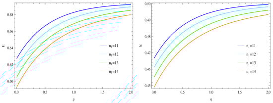
Figure 1. Von Neumann entropy (left panel) and negativity (right panel) versus the coupling constant $\eta$ for states n = 11–14 and $k=15$.

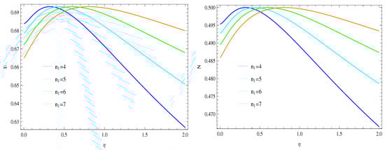
Figure 2. Von Neumann entropy (left panel) and negativity (right panel) versus the coupling constant $\eta$ for states n = 4–7 and $k=15$.

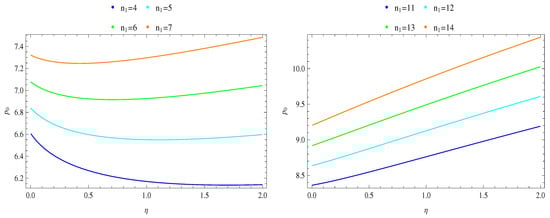
Figure 3. Total energy $p_0$ versus the coupling constant $\eta$ for states n = 4–7, n = 11–14, and $k=15$.

4. Conclusions

In this work, we have obtained exact solutions of the Dirac equation in the presence of Lorentz scalar linear potential and a monochromatic quantized electromagnetic plane wave. The resulting energy spectrum was found to contain a forbidden region that disappears when the particle–field interaction is absent, highlighting the nontrivial role of the quantized field in shaping the spectrum. We then examined the effect of particle–field coupling on the entanglement between the particle’s spin and its orbital-field degrees of freedom, using negativity and Von Neumann entropy as entanglement measures. A clear correlation was established between the energy profile of a given state and its entanglement behavior: when the total energy increases monotonically with the coupling, the spin–rest entanglement grows monotonically and saturates, while for states with non-monotonic energy, the entanglement exhibits a resonance-like peak before decreasing. This resonance reflects the competition between the scalar linear potential and the external field.

Our findings demonstrate how the interplay between external fields and confining potentials governs the redistribution of spinor amplitudes and, consequently, the pattern of quantum correlations. These insights may prove useful in the analysis of entanglement dynamics in relativistic quantum systems and in effective Dirac-like models such as graphene and trapped ions, where controllable couplings can be used to engineer entangled states.

References

- Fedorov, M.V. Atomic and Free Electrons in a Strong Laser Field; World Scientific: Singapore, 1997. [Google Scholar]
- Figueira de Morisson Faria, C.; Liu, X. Electron–electron correlation in strong laser fields. J. Mod. Opt. 2011, 58, 1076. [Google Scholar] [CrossRef]
- Volkov, D.M. Über eine klasse von lösungen der diracschen gleichung. Z. Phys. 1935, 94, 250. [Google Scholar]
- Gordon, W. Der comptoneffekt nach der schrödingerschen theorie. Z. Phys. 1926, 40, 117. [Google Scholar]
- Keldish, L.V. Ionization in the Field of a Strong Electromagnetic Wave. Zh. Eksp. Teor. Fiz. (USSR) 1964, 47, 1945. [Google Scholar]
- Ehlotzky, F.; Krajewska, K.; Kamiński, J.Z. Fundamental processes of quantum electrodynamics in laser fields of relativistic power. Rep. Prog. Phys. 2009, 72, 046401. [Google Scholar] [CrossRef]
- Zhang, L.-Q.; Liu, K.; Tang, S.; Luo, W.; Zhao, J.; Zhang, H.; Yu, T.-P. Generation of isolated and polarized γ-ray pulse by few-cycle laser irradiating a nanofoil. Rev. Mod. Plasma Phys. 2022, 64, 105011. [Google Scholar]
- Bagrov, V.G.; Baldiotti, M.C.; Gitmanc, D.M. Charged particles in crossed and longitudinal electromagnetic fields and beam guides. J. Math. Phys. 2007, 48, 082305. [Google Scholar] [CrossRef]
- Varró, S. New exact solutions of the Dirac equation of a charged particle interacting with an electromagnetic plane wave in a medium. Laser Phys. Lett. 2013, 10, 095301. [Google Scholar] [CrossRef][Green Version]
- Varró, S. A new class of exact solutions of the Klein–Gordon equation of a charged particle interacting with an electromagnetic plane wave in a medium. Laser Phys. Lett. 2014, 11, 016001. [Google Scholar]
- Raicher, E.; Eliezer, S.; Zigler, A. A novel solution to the Klein–Gordon equation in the presence of a strong rotating electric field. Phys. Lett. B 2015, 750, 76. [Google Scholar] [CrossRef][Green Version]
- Bagrov, V.G.; Gitmanc, D.M. Exact Solutions of Relativistic Wave Equation; Kluwer: Dordrecht, The Netherlands, 1990. [Google Scholar]
- Fedorov, M.V.; Kazakov, A.E. An electron in a quantized plane wave and in a constant magnetic field. Z. Phys. Hadrons Nucl. 1973, 261, 191–202. [Google Scholar] [CrossRef]
- Varró, S. Entangled photon–electron states and the number-phase minimum uncertainty states of the photon field. New J. Phys. 2008, 10, 053028. [Google Scholar] [CrossRef]
- Berson, I. Electron in the quantized field of a monochromatic electromagnetic wave. Zh. Eksp. Teor. Fiz. 1969, 56, 1627–1633. [Google Scholar]
- Bagrov, V.G.; Bozrikov, P.V.; Gitmanc, D.M. Electron in the field of a plane quantized electromagnetic wave. Teor. Mat. Fiz. 1973, 14, 202. [Google Scholar] [CrossRef]
- Bagrov, V.G.; Buchbinder, I.L.; Gitmanc, D.M.; Lavrov, P.M. Coherent states of an electron in a quantized electromagnetic wave. Teor. Mat. Fiz. 1977, 33, 419. [Google Scholar] [CrossRef]
- Berson, I.Y. Motion of an electron in an electromagnetic wave and a magnetic field parallel to it. AN Latv. SSR. Fiz. 1969, 5, 3. [Google Scholar]
- Abakarov, D.I.; Oleinik, V.P. Electron in the field of a quantized electromagnetic wave and in a homogeneous magnetic field. Teor. Mat. Fiz. 1972, 12, 673. [Google Scholar] [CrossRef]
- Guo, D.S.; Åberg, T. Quantum electrodynamical approach to multiphoton ionisation in the high-intensity H field. J. Phys. A 1988, 21, 4577. [Google Scholar] [CrossRef]
- Guo, D.S.; Åberg, T. Orthogonality and completeness of the quantum electrodynamical Volkov solutions. J. Phys. B 1991, 24, 349. [Google Scholar] [CrossRef]
- Guo, D.S.; Gao, J.; Chu, A.H.M. Relativistic electron moving in a multimode quantized radiation field. Phys. Rev. A 1996, 54, 1087. [Google Scholar] [CrossRef]
- Nielsen, M.; Chuang, E. Quantum Computation and Quantum Information; Cambridge University Press: Cambridge, UK, 2000. [Google Scholar]
- Bouwmeester, D.; Ekert, A.; Zeilinger, A. The Physics of Quantum Information; Springer: Berlin, Germany, 2000. [Google Scholar]
- Horodecki, R.; Horodecki, P.; Horodecki, M.; Horodecki, K. Quantum entanglement. Rev. Mod. Phys. 2009, 81, 865. [Google Scholar] [CrossRef]
- Bernardini, A.E.; Mizrahi, S.S. Relativistic dynamics compels a thermalized fermi gas to a unique intrinsic parity eigenstate. Phys. Scr. 2014, 89, 075105. [Google Scholar] [CrossRef][Green Version]
- Bittencourt, V.A.S.V.; Mizrahi, S.S.; Bernardini, A.E. SU(2) ⊗ SU(2) bi-spinor structure entanglement induced by a step potential barrier scattering in two-dimensions. Ann. Phys. 2015, 355, 35. [Google Scholar] [CrossRef][Green Version]
- Bittencourt, V.A.S.V.; Bernardini, A.E. Entanglement of Dirac bi-spinor states driven by Poincaré classes of SU(2) ⊗ SU(2) coupling potentials. Ann. Phys. 2016, 364, 182. [Google Scholar] [CrossRef]
- Bittencourt, V.A.S.V.; Bernardini, A.E.; Blasone, M. Quantum transitions and quantum entanglement from Dirac-like dynamics simulated by trapped ions. Phys. Rev. A 2016, 93, 053823. [Google Scholar] [CrossRef]
- Bittencourt, V.A.S.V.; Bernardini, A.E. Lattice-layer entanglement in Bernal-stacked bilayer graphene. Phys. Rev. B 2017, 95, 195145. [Google Scholar] [CrossRef]
- Hasegawa, Y.; Loidl, R.; Badurek, G.; Filipp, S.; Klepp, J.; Rauch, H. Evidence for entanglement and full tomographic analysis of Bell states in a single-neutron system. Phys. Rev. A 2007, 76, 052108. [Google Scholar] [CrossRef]
- Chargui, Y.; Trabelsi, A.; Chetouani, L. Exact solution of the (1 + 1)-dimensional Dirac equation with vector and scalar linear potentials in the presence of a minimal length. Phys. Lett. A 2010, 374, 531. [Google Scholar] [CrossRef]
- Gradshteyn, I.S.; Ryzhik, I.M. Table of Integrals, Series, and Products; Academic Press: Cambridge, MA, USA, 2007. [Google Scholar]
- Życzkowski, K.; Horodecki, P.; Sanpera, A.; Lewenstein, M. Volume of the set of separable states. Phys. Rev. A 1998, 58, 883. [Google Scholar] [CrossRef]
- Vidal, G.; Werner, R.F. Computable measure of entanglement. Phys. Rev. A 2002, 65, 032314. [Google Scholar] [CrossRef]
- Bennett, C.H.; Bernstein, H.J.; Popescu, S.; Schumacher, B. Concentrating partial entanglement by local operations. Phys. Rev. A 1996, 53, 2046. [Google Scholar] [CrossRef]
- Peres, A. Separability criterion for density matrices. Phys. Rev. Lett. 1996, 77, 1413. [Google Scholar] [CrossRef]
- Eltschka, C.; Siewert, J. Negativity as an estimator of entanglement dimension. Phys. Rev. Lett. 2013, 111, 100503. [Google Scholar] [CrossRef]
- Ekert, A.; Knight, P.L. Entangled quantum systems and the Schmidt decomposition. Am. J. Phys. 1995, 63, 415. [Google Scholar] [CrossRef]
- Costi, T.A.; McKenzie, R.H. Entanglement between a qubit and the environment in the spin-boson model. Phys. Rev. A 2003, 68, 034301. [Google Scholar] [CrossRef]
Disclaimer/Publisher’s Note: The statements, opinions and data contained in all publications are solely those of the individual author(s) and contributor(s) and not of MDPI and/or the editor(s). MDPI and/or the editor(s) disclaim responsibility for any injury to people or property resulting from any ideas, methods, instructions or products referred to in the content. |
© 2025 by the authors. Licensee MDPI, Basel, Switzerland. This article is an open access article distributed under the terms and conditions of the Creative Commons Attribution (CC BY) license (https://creativecommons.org/licenses/by/4.0/).