Quantum Simulation of Variable-Speed Multidimensional Wave Equations via Clifford-Assisted Pauli Decomposition

Abstract

The simulation of multidimensional wave propagation with variable material parameters is a computationally intensive task, with applications from seismology to electromagnetics. While quantum computers offer a promising path forward, their algorithms are often analyzed in the abstract oracle model, which can mask the high gate-level complexity of implementing those oracles. We present a framework for constructing a quantum algorithm for the multidimensional wave equation with a variable speed profile. The core of our method is a decomposition of the system Hamiltonian into sets of mutually commuting Pauli strings, paired with a dedicated diagonalization procedure that uses Clifford gates to minimize simulation cost. Within this framework, we derive explicit bounds on the number of quantum gates required for Trotter–Suzuki-based simulation. Our analysis reveals significant computational savings for structured block-model speed profiles compared to general cases. Numerical experiments in three dimensions confirm the practical viability and performance of our approach. Beyond providing a concrete, gate-level algorithm for an important class of wave problems, the techniques introduced here for Hamiltonian decomposition and diagonalization enrich the general toolbox of quantum simulation.

1. Introduction

Wave equations are fundamental for modeling a wide range of physical phenomena, from acoustic and seismic wave propagation to electromagnetic fields and quantum mechanics [1,2]. Numerically simulating these equations, especially in high dimensions and in the presence of heterogeneous material properties, remains computationally demanding for classical computers. While finite-difference and finite-element methods are widely used, they often suffer from the “curse of dimensionality”, where computational costs increase exponentially with the number of spatial dimensions [2,3]. This scaling imposes a significant bottleneck on applications requiring high-resolution models in three or more dimensions, such as full-waveform inversion in geophysics [4,5] or detailed optical simulations [6].

Quantum computing presents a promising avenue for overcoming these limitations. By exploiting the inherent parallelism of quantum states, quantum algorithms can achieve exponential speedups for certain linear algebra tasks and differential equation solvers [7,8]. Recent advancements have made significant strides in creating quantum algorithms tailored for partial differential equations (PDEs), notably the wave equation. Previous studies have demonstrated the efficacy of quantum algorithms employing an oracle to probe the wave speed profile [9,10]. In contrast, different studies have concentrated on more practical applications concerning one-dimensional scenarios where the speed remains constant [11,12,13]. An important challenge remains in creating clear, non-oracle methods for high-dimensional wave equations with changing speed coefficients, which are vital for accurate physical modeling. A recent study introduced an effective oracle-based solution for this task [14], employing an oracle technique that, while scalable, necessitates more ancilla qubits and incurs further overhead.

Our approach addresses this gap and builds on prior methods for Pauli decomposition of sparse matrices [15,16], extending them to arbitrary multidimensional wave problems with general and block-structured variable speed profiles. We derive explicit expressions for the number of Pauli strings, the structure of mutually commuting sets, and the corresponding diagonalization circuits. Exploiting these structures, we provide upper bounds on the number of one- and two-qubit gates required for first-order and higher-order Trotter approximations. Furthermore, by incorporating block-structured velocity profiles—common in practical applications such as layered media [5]—we demonstrate substantial reductions in circuit complexity, highlighting the advantage of leveraging problem-specific structure.

To support the theoretical scaling, we offer numerical simulations for a 3D wave equation featuring block-structured speed profiles. The results illustrate the effectiveness of our decomposition method and confirm the predicted scaling of Pauli term counts. Our analysis shows that the proposed quantum algorithm alleviates the classical “curse of dimensionality”, providing a practical approach to modeling wave dynamics in high-dimensional spaces.

The article begins by outlining the general problem of the multidimensional wave equation as framed for quantum algorithms in Section 2, including essential definitions. The main results are detailed in Section 3, with Section 3.1 covering Pauli decomposition, Section 3.2 focusing on diagonalization, Section 3.3 addressing the scaling of the multidimensional problem, and Section 3.4 examining the block speed scenario. Numerical simulations for the three-dimensional wave equation are presented in Section 3.5, followed by a discussion in Section 4 and concluding remarks in Section 5. Details on discretization and vectorization are provided in Appendix A; Appendix B contains the example of quantum algorithm construction, while Appendix C compares the classical finite difference approach with a developed algorithm in case of standing wave in terms of number of operations. Finally proofs of propositions are in Appendix D.

2. Materials and Methods

The wave equation set in D dimensions, characterized by variable speed and adhering to zero boundary conditions, is expressed as follows

$$\begin{array}{cc}\hfill & {\displaystyle \frac{{\partial }^{2}u(t,\overrightarrow{x})}{\partial t^2}}=\sum _{j=1}^D{\displaystyle \frac{\partial }{\partial x_j}}\left(c^2(\overrightarrow{x}){\displaystyle \frac{\partial u(t,\overrightarrow{x})}{\partial x_j}}\right),\hfill \\ \hfill & u(t=0,\overrightarrow{x})=f(\overrightarrow{x}),\hfill \\ \hfill & {\displaystyle \frac{\partial u(t=0,\overrightarrow{x})}{\partial t}}=g(\overrightarrow{x}),\hfill \\ \hfill & u(t,x_j=0)=0,j=1,\dots ,D,\hfill \\ \hfill & u(t,x_j=l_j)=0,j=1,\dots ,D.\hfill \end{array}$$

(1)

where $\overrightarrow{x}=(x_1,\dots ,x_D)$ and $l_j$ is the length of the corresponding dimension.

After discretization and vectorization denoted as $vec\left(·\right)$ (details are shown in Appendix A), we can write this in matrix–vector format as

$$\begin{array}{cc}\hfill & {\displaystyle \frac{{\partial }^2}{\partial t^2}}vec\left(U(t)\right)={\tilde{L}}_D(c(\overrightarrow{x}))vec\left(U(t)\right),\hfill \\ \hfill & vec\left(U(t=0)\right)=vec\left(F\right),\hfill \\ \hfill & {\displaystyle \frac{\partial }{\partial t}}vec\left(U(t=0)\right)=vec\left(G\right),\hfill \end{array}$$

(2)

where $U(t)$ is the tensor for the function $u(t,\overrightarrow{x})$ in a given domain, F is the tensor for the function $f(\overrightarrow{x})$ in a given domain, and G is the tensor for the function $g(\overrightarrow{x})$ in a given domain. The discrete operator is

$${\tilde{L}}_D(c(\overrightarrow{x}))=-\sum _{j=1}^D(I_1\otimes \cdots \otimes B_j\otimes \dots I_D)S^2(I_1\otimes \cdots \otimes B_j^T\otimes \dots I_D),$$

(3)

where S is the diagonal matrix with diagonal given by vectorized speed profile tensor C, which is discrete representation of $c(\overrightarrow{x})$ in a given domain, that is, $S=diag(vec\left(C\right))$, and $B_j$ is the first order forward first derivative approximation operator with explicit boundary conditions (first and last rows are zeros, as well as first and last columns). With this choice of $B_j$, the boundary conditions are incorporated into ${\tilde{L}}_D$.

2.1. Formulation as Schrödinger Equation

Following [9,16], consider the Schrödinger equation $i{\partial }_t\psi =H_D\psi$ using the Hamiltonian

$$H_D=\left(\begin{array}{cccccc}0& {\tilde{B}}_1& {\tilde{B}}_2& {\tilde{B}}_3& \dots & {\tilde{B}}_D\\ {\tilde{B}}_1^{†}& 0& 0& 0& \dots & 0\\ {\tilde{B}}_2^{†}& 0& 0& 0& \dots & 0\\ {\tilde{B}}_3^{†}& 0& 0& 0& \dots & 0\\ \dots & \dots & \dots & \dots & \dots & \dots \\ {\tilde{B}}_D^{†}& 0& 0& 0& \dots & 0\end{array}\right),$$

(4)

where ${\tilde{B}}_j=I_1\otimes \cdots \otimes B_j\otimes \cdots \otimes I_D$, with $B_j\in {\mathbb{R}}^{N\times N}$, $N=2^n$, being the matrix approximation of the first derivative with incorporated zero boundary conditions in a manner consistent with [16]. It is important to mention that typically, the size of matrix $B_j$ may vary across dimensions; however, for the present discussion, we assume it is the same. The matrices $\tilde{B}$ have the dimensions ${\mathbb{R}}^{N^D\times N^D}$, while the Hamiltonian $H_D$ is sized ${\mathbb{R}}^{(D+1)N^D\times (D+1)N^D}$. At present, we set $D+1=2^{n_D}$; extending this setup is straightforward since $H_D$ can be supplemented with zero matrices, which have no effect on the Pauli decomposition.

In order to incorporate a variable speed profile in this Hamiltonian, we consider

$${\tilde{H}}_D=\left(\begin{array}{cccccc}0& {\tilde{B}}_{1}S& {\tilde{B}}_{2}S& {\tilde{B}}_{3}S& \dots & {\tilde{B}}_{D}S\\ S{\tilde{B}}_1^{†}& 0& 0& 0& \dots & 0\\ S{\tilde{B}}_2^{†}& 0& 0& 0& \dots & 0\\ S{\tilde{B}}_3^{†}& 0& 0& 0& \dots & 0\\ \dots & \dots & \dots & \dots & \dots & \dots \\ S{\tilde{B}}_D^{†}& 0& 0& 0& \dots & 0\end{array}\right)=\tilde{S}{H}_D\tilde{S},\tilde{S}=diag(I,\underset{D}{\underbrace{S,\dots ,S}}),$$

(5)

where $S=diag(vec\left(C\right))$, and I is the identity matrix of the same size.

Differentiating the Schrödinger equation over time, given the Hamiltonian in (5), we get

$${\displaystyle \frac{d^2}{d{t}^2}}\left(\begin{array}{c}vec\left(U_V\right)\\ vec\left(G_1\right)\\ ⋮\\ vec\left(G_D\right)\end{array}\right)=-\left(\begin{array}{cccc}-{\tilde{L}}_D& 0& \dots & 0\\ 0& A_{11}& \dots & A_{1D}\\ ⋮& ⋮& \dots & ⋮\\ 0& A_{D1}& \dots & A_{DD}\end{array}\right)\left(\begin{array}{c}vec\left(U_V\right)\\ vec\left(G_1\right)\\ ⋮\\ vec\left(G_D\right)\end{array}\right),$$

(6)

where ${\tilde{L}}_D=-{\sum }_{j=1}^D{\tilde{B}}_j{S}^2{\tilde{B}}_j^{†}$, $vec\left(G_1\right),\dots ,vec\left(G_D\right)$ are some additional components in the wavefunction and $A_{ij}=S{\tilde{B}}_i^{†}{\tilde{B}}_{j}S$. Note that if matrix B is a finite difference approximation of the first derivative, then its negative transpose, and $-B^{†}$ is also an approximation. Specifically, $-B^{†}$ employs the mirror scheme: it yields a backward scheme if B uses a forward scheme, a forward scheme if B uses a backward scheme, and remains a central scheme if B is central. We can see now that the first component $vec\left(U_V\right)$ indeed evolves according to (2). One way to set the initial condition of the Schrödinger equation is

$$\begin{array}{cc}\hfill & vec\left(U_V(t=0)\right)=vec\left(F\right),\hfill \\ \hfill & vec\left(G_j(t=0)\right)={\displaystyle \frac{1}{D}}i{({\tilde{B}}_{j}S)}^{-1}vec\left(G\right),j=1,\dots D.\hfill \end{array}$$

(7)

Putting this together, the quantum algorithm for solving (1) reduces to preparing and evolving the state

$$|\psi (t)⟩=exp(-it{\tilde{H}}_D)|\psi (0)⟩,|\psi (t)⟩=\left(\begin{array}{c}vec\left(U_V\right)(t)\\ vec\left(G_1\right)(t)\\ ⋮\\ vec\left(G_D\right)(t)\end{array}\right).$$

(8)

We then postselect on the first component of ($|\psi (t)⟩$). While postselection, initialization, and the design of a suitable cost function are all very challenging tasks, in this work we focus on implementing the propagator $exp(-it{\tilde{H}}_D)$ using one- and two-qubit gates.

Remark 1.

If the right hand side of the wave Equation (1) is given by $c^2(\overrightarrow{x}){\sum }_{j=1}^D\left({\displaystyle \frac{{\partial }^{2}u(t,\overrightarrow{x})}{\partial x_j^2}}\right)$, one can use $\tilde{S}=diag(S,{{\displaystyle \underbrace{I,\dots ,I}}}_D)$ and consider the first component in the wavefunction as $vec\left(U_V\right)=S^{-1}vec\left(U_W\right)$. This way the component $vec\left(U_W\right)$ changes over time according to $L_D=-S^2{\sum }_{j=1}^D{\tilde{B}}_j{\tilde{B}}_j^{†}$, which is effectively a form of $c^2(\overrightarrow{x}){\sum }_{j=1}^D\left({\displaystyle \frac{{\partial }^{2}u(t,\overrightarrow{x})}{\partial x_j^2}}\right)$. Initial conditions in this case can be set as $vec\left(U_V(t=0)\right)=S^{-1}vec\left(F\right)$, and $vec\left(G_j(t=0)\right)={\displaystyle \frac{1}{D}}i{(S^2{\tilde{B}}_j)}^{-1}vec\left(G\right),j=1,\dots ,D$. This does not affect the results presented here since they are based on decompositions of S and $H_D$.

2.2. Propagator Implementation Technique

To execute the propagator $exp(-it{\tilde{H}}_D)$ on a quantum device, it must be broken down into operations that can be performed on such a device. This can be achieved by expressing ${\tilde{H}}_D$ as a sum of Pauli strings, which are tensor products of Pauli matrices, and then applying the Trotter formula [17,18]. For comprehensive definitions, the reader is directed to Section 2 of [15]; here, we will only present the key concepts.

To express Pauli strings with X and Z matrices, we use bit strings $\mathbf{z},\mathbf{x}\in {\mathbb{B}}^n$; with them, an arbitrary Pauli string can be defined as the image of the extended Pauli string operator (Walsh function) $\widehat{W}:{\mathbb{B}}^n\times {\mathbb{B}}^n\to {\mathcal{P}}_n$ as follows

$$\widehat{W}(\mathbf{x},\mathbf{z})={ı}^{\mathbf{x}·\mathbf{z}}{X}^{\mathbf{x}}{Z}^{\mathbf{z}}=\underset{j=1}{\overset{n}{⨂}}{ı}^{x_j{z}_j}{X}^{x_j}{Z}^{z_j},$$

(9)

with the matrix product between $X^{\mathbf{x}}$ and $Z^{\mathbf{z}}$ and $\mathbf{x}·\mathbf{z}={\sum }_{l=1}^n{x}_l{z}_l$ denoting the inner product of two bitstrings. It can be seen that the Walsh function is bijective. Thus, each Pauli string can be encoded with a unique pair $(\mathbf{x},\mathbf{z})$, and decomposition in the Pauli basis can be rewritten as

$${\tilde{H}}_D={\displaystyle \frac{1}{2^n}}\sum _{\mathbf{x},\mathbf{z}\in {\mathbb{B}}^n}{\beta }_{\mathbf{x},\mathbf{z}}\widehat{W}(\mathbf{x},\mathbf{z}),$$

(10)

where ${\beta }_{\mathbf{x},\mathbf{z}}\in \mathbb{C}$, and as shown in the proof of Proposition 4 of [15], the coefficients can be expressed in the form

$${\beta }_{\mathbf{x},\mathbf{z}}={ı}^{\mathbf{x}·\mathbf{z}}\sum _{\mathbf{p}\in \mathbb{B}}{(-1)}^{\mathbf{z}·\mathbf{p}}·h_{\mathbf{p},\mathbf{p}\oplus \mathbf{x}},$$

(11)

where ⊕ is a binary XOR (addition modulo 2) operation and $h_{\mathbf{p},\mathbf{p}\oplus \mathbf{x}}$ are elements of ${\tilde{H}}_D$, which makes it possible to compute coefficients in decomposition with $O(n{2}^n)$ operations.

As the strings in the decomposition do not all commute with each other, the Trotter formula can be utilized, offering different accuracy levels depending on the formula’s order. This approach is employed to manage the non-commutative characteristics of the operators involved in the decomposition. Building upon prior studies [15,16], we express ${\tilde{H}}_D$ as ${\sum }_{\gamma =1}^{\Gamma }{H}_{\gamma }$, where each $H_{\gamma }$ consists of mutually commuting Pauli strings. The Trotter formulas for orders 1, 2, and higher even orders $p=2k$, where $k=2,3,4,\dots$, are represented as

$$\begin{array}{cc}\hfill S_1(t)& =e^{-it{H}_{\Gamma }}\dots e^{-it{H}_1},\hfill \end{array}$$

(12)

$$\begin{array}{cc}\hfill S_2(t)& =e^{{\displaystyle \frac{-it}{2}}{H}_1}\dots e^{{\displaystyle \frac{-it}{2}}{H}_{\Gamma }}{e}^{{\displaystyle \frac{-it}{2}}{H}_{\Gamma }}\dots e^{{\displaystyle \frac{-it}{2}}{H}_1},\hfill \end{array}$$

(13)

$$\begin{array}{cc}\hfill S_{2k}(t)& =S_{2k-2}^2(s_{k}t)S_{2k-2}((1-4s_k)t)S_{2k-2}^2(s_{k}t),\hfill \end{array}$$

(14)

where $s_k=1/(4-4^{1/(2k-1)})$. The approximation accuracy is determined by the number of Trotterization steps r, the evolution time t, the order p of the Trotter formula, and the Hamiltonian norm.

3. Results

This section outlines our findings in the form of propositions and corollaries. We express the propagator for the multidimensional wave equation $exp(-it{\tilde{H}}_D)$ using single and two qubit operations as follows:

• We expand on the decomposition of Pauli strings as described in [16] to apply it to the wave equation in D dimensions (Proposition 1).
• We present a method for efficiently diagonalizing mutually commuting groups that emerge during decomposition (Proposition 2).
• We establish an upper bound and scaling on the complexity involved in solving the multidimensional wave equation with a variable speed profile using the Trotterization algorithm in terms of single- and two-qubit operations (Corollaries 2 and 3).
• We examine the practical scenario of a wave equation in D dimensions, characterized by a variable speed profile with a block structure and establish its upper bound and scaling (Corollary 4).
• We demonstrate the algorithm’s numerical performance on the three-dimensional wave equation with a block-structured speed profile (Section 3.5). We also compare the finite-difference method (FDM) with the quantum algorithm presented here for a three-dimensional standing wave, reporting the number of operations required to achieve the same accuracy (Appendix C).

3.1. Pauli String Decomposition

We extend the results presented in Proposition 1 from [16], particularly focusing on the case of a block Hamiltonian H with dimensions $(D+1)N\times (D+1)N$.

Proposition 1

(Decomposition of a block Hamiltonian). The only Pauli strings that can have non-zero coefficients in the decomposition of matrix

$$H=\left(\begin{array}{cccccc}0& B_1& B_2& B_3& \dots & B_D\\ B_1^{†}& 0& 0& 0& \dots & 0\\ B_2^{†}& 0& 0& 0& \dots & 0\\ B_3^{†}& 0& 0& 0& \dots & 0\\ \dots & \dots & \dots & \dots & \dots & \dots \\ B_D^{†}& 0& 0& 0& \dots & 0\end{array}\right),$$

(15)

where $B_p\in {\mathbb{C}}^{N\times N}$, $p=1,\dots ,D$, are d-diagonal matrices with $N=2^n$, described by $W({\mathbf{x}}_{p,k,j},\mathbf{z})$, where $\mathbf{z}\in {\mathbb{B}}^{n+|\widehat{\mathbb{B}}\left(D\right)|}$ and

$${\mathbf{x}}_{p,k,j}={\widehat{\mathbb{B}}}_l\left(|\widehat{\mathbb{B}}\left(D\right)|,p\right)\ast {\widehat{\mathbb{B}}}_l\left(n-s,2^j-1\right)\ast {\widehat{\mathbb{B}}}_l\left(s,2^s-k\right),$$

(16)

where $p\in \{1,\dots ,D\}$, $k\in \{1,\dots ,d\}$, $j\in \{1,\dots ,n-s\}$, $s=\lceil {log}_2(k)\rceil$, $d\le 2^{n-1}$. Moreover, the main diagonals of $B_p$ are represented by $W({\mathbf{x}}_{p,0},\mathbf{z})$, with 

$${\mathbf{x}}_{p,0}={\widehat{\mathbb{B}}}_l\left(|\widehat{\mathbb{B}}\left(D\right)|,p\right)\ast {\widehat{\mathbb{B}}}_l\left(n,0\right),$$

(17)

where $p\in \{1,\dots ,D\}$.

Here, function $|\widehat{\mathbb{B}}\left(D\right)|$ returns the number of bits necessary to represent D in binary form. Meanwhile, ${\widehat{\mathbb{B}}}_l\left(a,b\right)$ provides the binary form of b with a specified length a, padding with leading zeros if necessary. The symbol ∗ denotes the concatenation of binary strings.

It is noteworthy that if $D+1$ is not a power of 2, this proposition can still be utilized by appending matrices $B_p=0$ for $p=D+1,\dots ,D^{\prime }$, where $D^{\prime }$ is defined as $2^{\lceil {log}_2(D)\rceil }$. The d-diagonal matrices referenced in the proposition allow for enhanced accuracy of differential operators. Specifically, the three-diagonal matrices with d = 1 (where d denotes the count of diagonals above the main diagonal) will represent the first-order accurate differential operators.

All Pauli strings with non-zero coefficients in the decomposition are part of the sets labeled by ${\mathbf{x}}_{p,k,j}$ and ${\mathbf{x}}_{p,0}$, as described below:

$$\begin{array}{cc}\hfill S_{p,k,j}& =\{W({\mathbf{x}}_{p,k,j},\mathbf{z})|\mathbf{z}\in {\mathbb{B}}^{n+|\widehat{\mathbb{B}}\left(D\right)|}\},\hfill \\ \hfill S_{p,0}& =\{W({\mathbf{x}}_{p,0},\mathbf{z})|\mathbf{z}\in {\mathbb{B}}^{n+|\widehat{\mathbb{B}}\left(D\right)|}\}.\hfill \end{array}$$

(18)

In each set represented by ${\mathbf{x}}_{p,k,j}$ and ${\mathbf{x}}_0$, the elements are generated with $\mathbf{z}\in {\mathbb{B}}^{n+|\widehat{\mathbb{B}}\left(D\right)|}$, which are the binary representation of numbers from 0 to $2^{n+|\widehat{\mathbb{B}}\left(D\right)|}-1$ of length $n+|\widehat{\mathbb{B}}\left(D\right)|$. Therefore, the cardinality of each set is $2^{n+|\widehat{\mathbb{B}}\left(D\right)|}$. Furthermore, if $D+1$ is a power of 2, the cardinality can also be expressed as $(D+1)2^n$. Utilizing this proposition alongside Proposition 2 from [16], we formulate the ensuing corollary.

Corollary 1

(Number of sets in a block Hamiltonian). The total count of sets $S_{p,k,j}$ (including $S_{p,0}$) in the decomposition of Hamiltonian (15) with a d-band matrices $B_p\in {\mathbb{C}}^{N\times N},p=1,\dots ,D$, where $N=2^n$ is given by

$$s(D,d,n)=D\left(2^{|\widehat{\mathbb{B}}\left(d\right)|}+\left[n-|\widehat{\mathbb{B}}\left(d\right)|\right]d\right),$$

(19)

where $|\widehat{\mathbb{B}}\left(d\right)|$ is the binary length of d.

We group the sets from Equation (18) into mutually commuting subsets, a result that aligns with previous findings [15,16].The assignment to a subset is determined by whether a Pauli string contains an odd or even number of Y matrices (i.e., the value of $\mathbf{x}·\mathbf{z}mod2$), as stated in Corollary 2 of [16]. In the specific case of a real-valued matrix, all Pauli strings have an even number of Y matrices, which leads to $s(D,d,n)$ mutually commuting sets.

3.2. Mutual Diagonalization

In Proposition 1 we have provided strings ${\mathbf{x}}_{p,k,j}$, which generate mutually commuting sets based on parity of Y operators (value of $\mathbf{x}·\mathbf{z}(\mathrm{mod}2)$). We outline the diagonalization process for these sets, drawing upon [19,20], and present it as the subsequent proposition.

Proposition 2

(Diagonalization of sets). Given the set of mutually commuting operators, characterized by a string $\mathbf{x}\in {\mathbb{B}}^n$, that is, $\{W(\mathbf{x},\mathbf{z})|\mathbf{z}\in {\mathbb{B}}^n,\mathbf{x}·\mathbf{z}=0(\mathrm{mod}2)\},$ or $\{W(\mathbf{x},\mathbf{z})|\mathbf{z}\in {\mathbb{B}}^n,\mathbf{x}·\mathbf{z}=1(\mathrm{mod}2)\},$ one can construct diagonalization operator $\widehat{D}$, such that $W(\mathbf{x},\mathbf{z})={(-1)}^r{\widehat{D}}^{†}W(\mathbf{0},\tilde{\mathbf{z}})\widehat{D}$, with $r=\left({\displaystyle \frac{\mathbf{x}·\mathbf{z}+(\mathbf{x}·\mathbf{z}mod2)}{2}}\right)$ as

$$\begin{array}{cc}\hfill \widehat{D}& =H_{k_1}\prod _{j=2}^{M}CNOT(k_1,k_j),if\mathbf{x}·\mathbf{z}=0(\mathrm{mod}2),\hfill \\ \hfill \widehat{D}& =H_{k_1}{S}_{k_1}\prod _{j=2}^{M}CNOT(k_1,k_j),if\mathbf{x}·\mathbf{z}=1(\mathrm{mod}2),\hfill \end{array}$$

(20)

where $CNOT(c,t)$ is a controlled-NOT operation with control on the c-th qubit and target on the t-th qubit; $H_k$ and $S_k$ are Hadamard and phase gates acting on the k-th qubit, respectively. The product runs over all indices $k_j$ of the nonzero bits in $\mathbf{x}$, where M is the total number of these bits and $k_1$ is the index of the first nonzero bit. This procedure yields the string $\tilde{\mathbf{z}}$, which is identical to $\mathbf{z}$ except that its $k_1$-th bit is set to 1.

This proposition enables the diagonalization of any set of mutually commuting operators using only the corresponding string $\mathbf{x}$. The number of one- and two-qubit gates required for this diagonalization is determined by the parity of $\mathbf{x}·\mathbf{z}$: it is M if $\mathbf{x}·\mathbf{z}=0mod2$ and $M+1$ if $\mathbf{x}·\mathbf{z}=1mod2$, where M is the number of nonzero bits (Hamming weight) in $\mathbf{x}$. Additionally, the proposition provides the outcome of the diagonalization, that is, string $\tilde{\mathbf{z}}$.

3.3. Scaling of Multidimensional Wave Equation Quantum Algorithm

Using general results presented in previous sections, we formulate the following proposition made specifically for the multidimensional wave equation.

Proposition 3

(Decomposition of multidimensional wave equation Hamiltonian). The Hamiltonian for the D-dimensional wave problem stated as (1) can be written as

$${\tilde{H}}_D=\left(\begin{array}{cccccc}0& {\tilde{B}}_{1}S& {\tilde{B}}_{2}S& {\tilde{B}}_{3}S& \dots & {\tilde{B}}_{D}S\\ S{\tilde{B}}_1^{†}& 0& 0& 0& \dots & 0\\ S{\tilde{B}}_2^{†}& 0& 0& 0& \dots & 0\\ S{\tilde{B}}_3^{†}& 0& 0& 0& \dots & 0\\ \dots & \dots & \dots & \dots & \dots & \dots \\ S{\tilde{B}}_D^{†}& 0& 0& 0& \dots & 0\end{array}\right)=\tilde{S}{H}_D\tilde{S},\tilde{S}=diag(I,\underset{D}{\underbrace{S,\dots ,S}}),$$

(21)

where ${\tilde{B}}_j=I_1\otimes \dots \otimes B_j\otimes \dots I_D$ with $B_j\in {\mathbb{R}}^{N\times N},j=1,\dots ,D$ - d-diagonal matrices, with $N=2^n$, and diagonal matrix $S\in {\mathbb{R}}^{N^D\times N^D}$. Given Pauli decomposition $\tilde{S}={\sum }_{j=1}^T{\alpha }_j{Z}^{{\mathbf{z}}_j}$, where $Z^{\mathbf{z}}={⨂}_{k=1}^{Dn+|\widehat{\mathbb{B}}\left(D\right)|}{Z}^{z_k}$, with $z_k$ being the k-th bit in $\mathbf{z}$, the number of Pauli strings that can have non-zero coefficients in the decomposition of matrix ${\tilde{H}}_D$ is bounded by $g_H\le \Gamma min(T^{2}K,(D+1)N^D/2)$, where $\Gamma$ is the number of mutually commuting sets in $H_D$, and K is the number of Pauli strings in the single set. T is the number of Pauli strings in the decomposition of $\tilde{S}$.

The Hamiltonian $H_D$ can be directly subjected to Proposition 1 and Corollary 1 with no alterations. The form of the Pauli strings in the decomposition remains essentially the same. To convert H into $H_D$, one simply needs to insert extra identity (I) matrices at the qubit locations that align with the structure of the ${\tilde{B}}_j$ operators. In the binary representation of the Pauli strings using vectors $\mathbf{x}$ and $\mathbf{z}$, this operation corresponds to adding zeros at the appropriate bit locations.

It is also observed that the number of mutually commuting sets in ${\tilde{H}}_D$ is identical to that in $H_D$ because $\tilde{S}$ represents a diagonal matrix. According to Corollary 1, this count is denoted by $\Gamma =s(D,d,n)$, owing to the real-valued nature of $H_D$. If the number of diagonals d above the main is significantly less than N, a situation common with finite difference approximation matrices $B_j$, the number of commuting sets can be approximated by $\Gamma =O(Ddn)$. The count of Pauli strings K contained within a single commuting set can be bounded by $K\le 2^{n+|\widehat{\mathbb{B}}\left(D\right)|-1}=(D+1)N/2$ since only strings with an even number of Y Pauli matrices participate in the decomposition. Consequently, the overall number of Pauli strings that appear in ${\tilde{H}}_D=\tilde{S}{H}_D\tilde{S}$ can be expressed as $O(D^{2}dnNmin(T^2,N^{D-1}))$, where T denotes the number of Pauli strings used in the decomposition of $\tilde{S}$. Furthermore, in cases where $T^2\le N^{D-1}$, the estimation may be modified to

$$g_H=O(D^{2}dn{T}^{2}N).$$

(22)

From this result, we can estimate the number of one- and two-qubit gates required for a single Trotter step that realizes the time evolution operator $exp(-i{\tilde{H}}_{D}t)$. The construction of one Trotter step requires the diagonalization of each of the $s(D,d,n)$ mutually commuting sets of Pauli strings. Recall that a Pauli string $\mathbf{x}$ can contain non-zero bits solely within the initial $|\widehat{\mathbb{B}}\left(D\right)|$ places and the n locations specified by j in ${\tilde{B}}_j=I_1\otimes \cdots \otimes B_j\otimes \dots I_D$. Based on Proposition 2 and given the condition $\mathbf{x}·\mathbf{z}\equiv 0(mod2)$, the count of one- and two-qubit gates necessary for the diagonalization and reverse diagonalization of a single set is limited by

$$g_d\le 2(n+|\widehat{\mathbb{B}}\left(D\right)|).$$

(23)

Diagonalized Pauli strings are composed solely of Z operators. These can be executed using multi-qubit rotations denoted by $R_{\tilde{\mathbf{z}}}(\theta )\equiv exp\left(-i{\displaystyle \frac{\theta }{2}}{Z}^{\tilde{\mathbf{z}}}\right)$, where $\tilde{\mathbf{z}}$ represents the modified string $\mathbf{z}$ in each respective diagonal group. The sequence of these rotations is organized in such a way as to optimize their implementation by reducing the number of CNOT gates required, achieved through minimizing the Hamming distance between successive $\tilde{\mathbf{z}}$ strings [21] (see a circuit example for a single group in Appendix B). Without particular assumptions about the configuration of $\tilde{S}$, we employ a worst-case scenario in which every $\tilde{\mathbf{z}}$ sequence is composed entirely of ones, with no cancellations occurring. This provides an upper limit of $2(Dn+|\widehat{\mathbb{B}}\left(D\right)|-1)$ CNOT gates for each rotation since the maximum number of CNOTs needed for an m-qubit rotation is $2(m-1)$ [21]. Hence, the total number of gates necessary for realizing all rotations within a single diagonal configuration is bounded by $g_z\le 2\left(Dn+|\widehat{\mathbb{B}}\left(D\right)|\right)min(T^{2}K,(D+1)N^D/2)$.

By bringing these components together, the total number $g_1$ of one- and two-qubit gates required for each single step of the first-order Trotter–Suzuki decomposition to approximate $exp(-i{\tilde{H}}_{D}t)$ is constrained by

$$g_1\le \Gamma ·(g_d+g_z),$$

(24)

where

• $\Gamma =s(D,d,n)=D\left(2^{|\widehat{\mathbb{B}}\left(d\right)|}+\left(n-|\widehat{\mathbb{B}}\left(d\right)|\right)d\right)$ represents the number of sets of Pauli strings that internally mutually commute;
• $g_d\le 2(n+|\widehat{\mathbb{B}}\left(D\right)|)$ is the gate count for diagonalization operators per set;
• $g_z\le (Dn+|\widehat{\mathbb{B}}\left(D\right)|)(D+1)Nmin(T^2,N^{D-1})$ represents the gate count for implementing the diagonal rotations per set. We relied on the estimation $K\le (D+1)N/2$ as suggested by Proposition 1.

Therefore, the explicit bound in case $T^2<N^{D-1}$ for one step of first order Trotter formula is

$$g_1\le s(D,d,n)\left[2\left(n+|\widehat{\mathbb{B}}\left(D\right)|\right)+\left(Dn+|\widehat{\mathbb{B}}\left(D\right)|\right)N(D+1)T^2\right].$$

(25)

For higher-order Trotter–Suzuki formulas of even order p [17,18], the gate count scales as

$$g_p=2·5^{\lfloor p/2\rfloor -1}{g}_1,\mathrm{for}p=2,4,6,\dots$$

(26)

We formalize the scaling for a single Trotter step in the following corollary.

Corollary 2

(One Trotter step scaling). Given the Hamiltonian

$${\tilde{H}}_D=\left(\begin{array}{cccccc}0& {\tilde{B}}_{1}S& {\tilde{B}}_{2}S& {\tilde{B}}_{3}S& \dots & {\tilde{B}}_{D}S\\ S{\tilde{B}}_1^{†}& 0& 0& 0& \dots & 0\\ S{\tilde{B}}_2^{†}& 0& 0& 0& \dots & 0\\ S{\tilde{B}}_3^{†}& 0& 0& 0& \dots & 0\\ \dots & \dots & \dots & \dots & \dots & \dots \\ S{\tilde{B}}_D^{†}& 0& 0& 0& \dots & 0\end{array}\right)=\tilde{S}{H}_D\tilde{S},\tilde{S}=diag(I,\underset{D}{\underbrace{S,\dots ,S}}),$$

(27)

where ${\tilde{B}}_j=I_1\otimes \cdots \otimes B_j\otimes \dots I_D$ with $B_j\in {\mathbb{R}}^{N\times N},j=1,\dots ,D$ - d-diagonal matrices, with $N=2^n$, and diagonal matrix $\tilde{S}={\sum }_{j=1}^T{\alpha }_j{Z}^{{\mathbf{z}}_j}\in {\mathbb{R}}^{N^D\times N^D}$ with T strings in decomposition. The number of one- and two-qubit gates for one step of first order Trotter formula for $exp(-i{\tilde{H}}_{D}t)$ with assumptions $d\ll N$ and $T^2<N^{D-1}$ scales as

$$\begin{array}{cc}\hfill & g_1=O\left(D^{3}d{n}^{2}N{T}^2\right)\hfill \\ \hfill & g_p=O\left(5^{\lfloor p/2\rfloor }{D}^{3}d{n}^{2}N{T}^2\right),p=2,4,6\dots .\hfill \end{array}$$

(28)

This process can be made more efficient with a few methods. To start, the Hamming distance between neighboring bitstrings $\tilde{\mathbf{z}}$ should be reduced. This configuration aids in eliminating CNOT gates used for executing the multi-qubit $R_{\tilde{\mathbf{z}}}$ rotations. Secondly, an analogous improvement is realized by tactically reordering the sets, which facilitates the elimination of CNOT gates produced during the diagonalization process. Moreover, the arrangement of these sets constituting $\tilde{S}$ can be utilized to lessen the number of gates, as illustrated in Section 3.4.

Finally, by employing Corollary 2, we shall illustrate the scaling of one- and two-qubit gates required for executing the propagator $exp(-i{\tilde{H}}_{D}t)$ using the Trotter formula of order p. The scaling can be expressed as $g_{tr}=g_{p}r$, where $g_p$ denotes the count of gates per trotter step of p-th order, and r represents the total number of steps needed to achieve an error of $ϵ={exp(-i{\tilde{H}}_{D}t)-U(t,r,p)}_2$. In this context, $U(t,r,p)$ serves as the Trotter approximation for $exp(-i{\tilde{H}}_{D}t)$. To determine r, we utilize the scaling outlined by the authors in [17], specifically

$$r=O\left({\left(2\Gamma 5^{\lfloor p/2\rfloor -1}{\tilde{H}}_{D}t\right)}^{1+1/p}{(1/ϵ)}^{1/p}\right),$$

(29)

where $\Gamma$ denotes the quantity of easy to implement Hamiltonians (in our case, we choose it to be mutually commuting sets) within ${\tilde{H}}_D$. We can approximate the Hamiltonian norm by ${\tilde{H}}_D=O(dN)$ because the matrices $B_j$ in ${\tilde{H}}_D$ function as finite difference operators, which inherently contain the inverse of the discretization step size $1/h=O(N)$. The subsequent corollary outlines the scaling requirements essential for constructing a quantum circuit that sets up the propagator for the D-dimensional wave equation, denoted as $exp(-i{\tilde{H}}_{D}t)$, with a margin of error $ϵ$.

Corollary 3

(Scaling for multidimensional wave equation quantum algorithm). Given the Hamiltonian for D-dimensional wave equation as

$${\tilde{H}}_D=\left(\begin{array}{cccccc}0& {\tilde{B}}_{1}S& {\tilde{B}}_{2}S& {\tilde{B}}_{3}S& \dots & {\tilde{B}}_{D}S\\ S{\tilde{B}}_1^{†}& 0& 0& 0& \dots & 0\\ S{\tilde{B}}_2^{†}& 0& 0& 0& \dots & 0\\ S{\tilde{B}}_3^{†}& 0& 0& 0& \dots & 0\\ \dots & \dots & \dots & \dots & \dots & \dots \\ S{\tilde{B}}_D^{†}& 0& 0& 0& \dots & 0\end{array}\right)=\tilde{S}{H}_D\tilde{S},\tilde{S}=diag(I,\underset{D}{\underbrace{S,\dots ,S}}),$$

(30)

where ${\tilde{B}}_j=I_1\otimes \cdots \otimes B_j\otimes \dots I_D$ with $B_j\in {\mathbb{R}}^{N\times N},j=1,\dots ,D$ - d-diagonal matrices, with $N=2^n$, and diagonal matrix $\tilde{S}={\sum }_{j=1}^T{\alpha }_j{Z}^{{\mathbf{z}}_j}\in {\mathbb{R}}^{N^D\times N^D}$ with T strings in decomposition, the number of one- and two-qubit gates required to implement a p-th order Trotter approximation $U(t,r,p)$ with r steps, satisfying ${e^{-i{\tilde{H}}_{D}t}-U(t,r,p)}_2\le ϵ$ scales as

$$g_{tr}=O\left(t{5}^p{D}^4{d}^3{n}^3{N}^2{T}^2{\left({\displaystyle \frac{2}{5}}D{d}^{2}nNt/ϵ\right)}^{1/p}\right),$$

(31)

assuming $d\ll N$ and $T^2<N^{D-1}$.

The suggested approach mitigates the “curse of dimensionality” in a manner similar to the oracle-based method discussed in [9]. According to Corollary 2, the gate complexity for one Trotter step predominantly scales with the $N{T}^2$ factor, which varies linearly with the system size, where $N=2^n$. Nevertheless, the total complexity is primarily determined by the number of steps needed to reach the desired precision. When utilizing a p-th order Trotter formula, the dominant scaling factor is $N^{2+1/p}{T}^2$. The extra scaling related to N stems from the finite difference approximation, which requires a step size that is contingent upon N.

3.4. Scaling of Multidimensional Wave Equation Quantum Algorithm with Block-Model Speed Profile

In this section, we adopt a block-model representation in which the domain is partitioned into regions of constant wave speed (acoustic approximation). This assumption is widely used because it simplifies the forward problem, provides clear correspondence between model parameters and geological interfaces, and enables efficient numerical implementation. However, it should be noted that real Earth materials rarely consist of perfectly homogeneous blocks. In practice, velocity and density typically vary smoothly due to compaction, mineral composition, and fluid content, and fine-scale heterogeneity introduces scattering and waveform complexity that are not captured in block models [22]. As a result, the block approximation can overestimate reflection amplitudes at sharp interfaces and underestimate energy redistribution into scattered or coda waves. Nevertheless, when seismic wavelengths are large relative to heterogeneity scales, block models offer a reasonable first-order description of wave kinematics, particularly for traveltime and phase analyses.

Consider a computational domain of size $2^{n_x}\times 2^{n_y}\times 2^{n_z}$, discretized uniformly into $2^{m_x}$, $2^{m_y}$, and $2^{m_z}$ segments along the x, y, and z axes, respectively. The total number of distinct material blocks, and thus the number of independent variables in the system, is given by $T=2^{m_x+m_y+m_z}$. Moreover, the vectorized velocity profile $S=diag(vec(C))$, with C being a tensor representation of $c(\overrightarrow{x})$, can be expressed as a linear combination of Pauli operators as follows:

$$S=\sum _{\begin{array}{c}{\mathbf{z}}_x\in {\mathbb{B}}^{m_x},\\ {\mathbf{z}}_y\in {\mathbb{B}}^{m_y},\\ {\mathbf{z}}_z\in {\mathbb{B}}^{m_z}\end{array}}{\alpha }_{{\mathbf{z}}_x,{\mathbf{z}}_y,{\mathbf{z}}_z}\underset{n_x}{\underbrace{Z^{{\mathbf{z}}_x}\otimes I^{\otimes n_x-m_x}}}\otimes \underset{n_y}{\underbrace{Z^{{\mathbf{z}}_y}\otimes I^{\otimes n_y-m_y}}}\otimes \underset{n_z}{\underbrace{Z^{{\mathbf{z}}_z}\otimes I^{\otimes n_z-m_z}}},$$

(32)

where $Z^{\mathbf{z}}={⨂}_{k=1}{Z}^{z_k}$, with $z_k$ being the k-th bit in $\mathbf{z}$. This formulation demonstrates that the operator S is decomposed into a sum of T Pauli terms. Each term corresponds to a diagonal Pauli string (composed of I and Z operators) acting on the $m=m_x+m_y+m_z$ qubits that encode the model parameterization, while identity operators act on the remaining $(n_x+n_y+n_z-m)$ qubits that correspond to a size of block in particular direction.

The number of terms in this decomposition is precisely equal to the number of variables, T, and the generalization to the multidimensional case is straightforward. To estimate the gate complexity of implementing the operator $\tilde{S}$, one must account for an ancillary register of size $\lceil {log}_2(D+1)\rceil =|\widehat{\mathbb{B}}\left(D\right)|$ qubits. Crucially, the block structure of S given by Equation (32) provides a significant reduction in computational complexity. We leverage this by reformulating Corollaries 2 and 3 for the block-model speed profile.

Corollary 4

(Scaling for block-model speed profile). Given the Hamiltonian

$${\tilde{H}}_D=\left(\begin{array}{cccccc}0& {\tilde{B}}_{1}S& {\tilde{B}}_{2}S& {\tilde{B}}_{3}S& \dots & {\tilde{B}}_{D}S\\ S{\tilde{B}}_1^{†}& 0& 0& 0& \dots & 0\\ S{\tilde{B}}_2^{†}& 0& 0& 0& \dots & 0\\ S{\tilde{B}}_3^{†}& 0& 0& 0& \dots & 0\\ \dots & \dots & \dots & \dots & \dots & \dots \\ S{\tilde{B}}_D^{†}& 0& 0& 0& \dots & 0\end{array}\right)=\tilde{S}{H}_D\tilde{S},\tilde{S}=diag(I,\underset{D}{\underbrace{S,\dots ,S}}),$$

(33)

where ${\tilde{B}}_j=I_1\otimes \cdots \otimes B_j\otimes \dots I_D$ with $B_j\in {\mathbb{R}}^{N\times N},j=1,\dots ,D$ - d-diagonal matrices, with $N=2^n$, and a real diagonal matrix S, given as

$$S=\sum _{{\mathbf{z}}_j\in {\mathbb{B}}^m,j=1,\dots ,D}{\alpha }_{{\mathbf{z}}_j,\dots ,{\mathbf{z}}_D}\underset{n}{\underbrace{Z^{{\mathbf{z}}_1}\otimes I^{\otimes n-m}}}\otimes \cdots \otimes \underset{n}{\underbrace{Z^{{\mathbf{z}}_D}\otimes I^{\otimes n-m}}}.$$

(34)

The number of one- and two-qubit gates for one step of first order Trotter formula for $exp(-i{\tilde{H}}_{D}t)$ with assumption $d\ll N$ scales as

$$\begin{array}{cc}\hfill & g_1=O\left(D^{2}dnN{2}^{(D-1)m}\right)\hfill \\ \hfill & g_p=O\left(5^{\lfloor p/2\rfloor }{D}^{2}dnN{2}^{(D-1)m}\right),p=2,4,6\dots .\hfill \end{array}$$

(35)

Consequently, under the same assumptions the number of one- and two-qubit gates required to implement a p-th order Trotter approximation $U(t,r,p)$ with r steps, satisfying ${e^{-i{\tilde{H}}_{D}t}-U(t,r,p)}_2\le ϵ$, scales as

$$g_{tr}=O\left(t{5}^p{D}^3{d}^3{n}^2{N}^2{2}^{(D-1)m}{\left({\displaystyle \frac{2}{5}}D{d}^{2}nNt/ϵ\right)}^{1/p}\right).$$

(36)

The manner in which the system scales is dictated by the configuration of the resulting sets of Pauli operators. According to Proposition 1, one can systematically generate the entire set of possible bit strings $\mathbf{x}$.

Given a binary string $\mathbf{x}$, the strings $\mathbf{z}$ are formulated in the following manner:

• In the case where $m=0$, the non-zero elements of the $\mathbf{z}$ strings are constrained to the positions directly specified by the structure of the matrix ${\tilde{B}}_j$. For example, given ${\tilde{B}}_1=B\otimes I\otimes \cdots \otimes I$, the Pauli strings associated with ${\tilde{B}}_1$ are the same as in decomposition of B but are padded with identity operators (I). This corresponds to appending zeros to both the $\mathbf{x}$ and $\mathbf{z}$ strings.
• For a general parameter $m\ge 0$, if the velocity profile adheres to the structure defined in Equation (34), the number of positions in the $\mathbf{z}$ strings that can support non-zero values increases. Specifically, an additional $Dm$ bits must be considered. These correspond to the first m bits in each of the D spatial directions within the $\mathbf{z}$ string.

Therefore, the number of Pauli strings in a single set can be bounded as $K^{\prime }\le 2^{n+|\widehat{\mathbb{B}}\left(D\right)|+(D-1)m-1}$, where the term $(D-1)m$ appears because, for a single dimension in the considered set, all bits are already accounted for in the implementation of B. Moreover, in this scenario, Gray code ordering can be applied within each mutually commuting set, allowing the elimination of certain CNOT gates and thus reducing the number of gates required to implement rotations for a single group to $g_z\le 2K^{\prime }$.

To illustrate this we present the full set of strings $\mathbf{x}$ and corresponding masks for $\mathbf{z}$ as described above for a three-dimensional wave equation—discretized with 2 qubits per dimension and with finite difference operators approximated by tridiagonal matrices ($d=1$) in Table 1 for different values of m.

Table 1. Example of all possible Pauli strings for the three-dimensional wave equation, discretized with 2 qubits per dimension and with finite difference operators approximated by tridiagonal matrices ($d=1$). The strings ${\mathbf{x}}_{p,k,j}$ (where $k=1$ due to $d=1$) are generated according to Proposition 1. The corresponding masks for the $\mathbf{z}$ strings are shown for different values of m in the block speed model; a “∗” denotes a position that can be either 0 or 1. Bits are grouped for readability: the first $|\widehat{\mathbb{B}}\left(D\right)|=2$ bits are used for the Hamiltonian construction, and each subsequent block of $n=2$ bits encodes a spatial direction.

${\mathbf{x}}_{\mathit{p},1,\mathit{j}}$	z, $\mathit{m}=0$	z, $\mathit{m}=1$	z, $\mathit{m}=2$
${\mathbf{x}}_{1,0}=01|00|00|00$	$\mathbf{z}=\ast \ast |\ast \ast |00|00$	$\mathbf{z}=\ast \ast |\ast \ast |\ast 0|\ast 0$	$\mathbf{z}=\ast \ast |\ast \ast |\ast \ast |\ast \ast$
${\mathbf{x}}_{1,1,1}=01|01|00|00$	$\mathbf{z}=\ast \ast |\ast \ast |00|00$	$\mathbf{z}=\ast \ast |\ast \ast |\ast 0|\ast 0$	$\mathbf{z}=\ast \ast |\ast \ast |\ast \ast |\ast \ast$
${\mathbf{x}}_{1,1,2}=01|11|00|00$	$\mathbf{z}=\ast \ast |\ast \ast |00|00$	$\mathbf{z}=\ast \ast |\ast \ast |\ast 0|\ast 0$	$\mathbf{z}=\ast \ast |\ast \ast |\ast \ast |\ast \ast$
${\mathbf{x}}_{2,0}=10|00|00|00$	$\mathbf{z}=\ast \ast |00|\ast \ast |00$	$\mathbf{z}=\ast \ast |\ast 0|\ast \ast |\ast 0$	$\mathbf{z}=\ast \ast |\ast \ast |\ast \ast |\ast \ast$
${\mathbf{x}}_{2,1,1}=10|00|01|00$	$\mathbf{z}=\ast \ast |00|\ast \ast |00$	$\mathbf{z}=\ast \ast |\ast 0|\ast \ast |\ast 0$	$\mathbf{z}=\ast \ast |\ast \ast |\ast \ast |\ast \ast$
${\mathbf{x}}_{2,1,2}=10|00|11|00$	$\mathbf{z}=\ast \ast |00|\ast \ast |00$	$\mathbf{z}=\ast \ast |\ast 0|\ast \ast |\ast 0$	$\mathbf{z}=\ast \ast |\ast \ast |\ast \ast |\ast \ast$
${\mathbf{x}}_{3,0}=11|00|00|00$	$\mathbf{z}=\ast \ast |00|00|\ast \ast$	$\mathbf{z}=\ast \ast |\ast 0|\ast 0|\ast \ast$	$\mathbf{z}=\ast \ast |\ast \ast |\ast \ast |\ast \ast$
${\mathbf{x}}_{3,1,1}=11|00|00|01$	$\mathbf{z}=\ast \ast |00|00|\ast \ast$	$\mathbf{z}=\ast \ast |\ast 0|\ast 0|\ast \ast$	$\mathbf{z}=\ast \ast |\ast \ast |\ast \ast |\ast \ast$
${\mathbf{x}}_{3,1,2}=11|00|00|11$	$\mathbf{z}=\ast \ast |00|00|\ast \ast$	$\mathbf{z}=\ast \ast |\ast 0|\ast 0|\ast \ast$	$\mathbf{z}=\ast \ast |\ast \ast |\ast \ast |\ast \ast$

The number of $\mathbf{z}$ strings that must be considered can be reduced by leveraging the decomposition of the specific matrix $H_D$. However, in this work, we consider an arbitrary diagonal structure as a more general approach that enables the explicit encoding of boundary conditions, as demonstrated in [16].

3.5. A Three-Dimensional Wave Equation in a Numerical Example

As a practical example of our approach, we conducted a numerical simulation focusing on the three-dimensional wave Equation ($D=3$). A finite-difference scheme is employed to discretize the problem on a regular grid, with each spatial dimension depicted by n qubits, leading to $N=2^n$ grid points for each dimension. The tridiagonal ($d=1$) matrices provide an approximation for the finite-difference operators, and we utilize the block speed model described in Equation (32). The task at hand involves computing the implementation of the propagator $exp(-it{\tilde{H}}_3)$, where the Hamiltonian ${\tilde{H}}_3$ is defined as

$${\tilde{H}}_3=\left(\begin{array}{cccc}0& {\tilde{B}}_{x}S& {\tilde{B}}_{y}S& {\tilde{B}}_{z}S\\ S{\tilde{B}}_x^T& 0& 0& 0\\ S{\tilde{B}}_y^T& 0& 0& 0\\ S{\tilde{B}}_z^T& 0& 0& 0\end{array}\right)=\tilde{S}{H}_3\tilde{S},\tilde{S}=\left(\begin{array}{cccc}I& 0& 0& 0\\ 0& S& 0& 0\\ 0& 0& S& 0\\ 0& 0& 0& S\end{array}\right),$$

(37)

with ${\tilde{B}}_x=B\otimes I\otimes I$, ${\tilde{B}}_y=I\otimes B\otimes I$, ${\tilde{B}}_z=I\otimes I\otimes B$. Here, $B,I\in {\mathbb{R}}^{N\times N}$, and B is a tridiagonal matrix incorporating zero boundary conditions [15].

Direct classical simulation of $exp(-it{\tilde{H}}_3)$ is computationally hard. For instance, a discretization with $n=6$ qubits ($N=64$ points) per dimension requires exponentiating a matrix of size $4N^3=2^{3n+2}=2^{20}\approx {10}^6$. For realistic scenarios requiring high resolution (e.g., $n\ge 10$, or $N\ge 1000$ points per dimension), direct classical computation of the propagator becomes intractable.

For this physically meaningful resolutions—e.g., $n\ge 10$ so $N=2^{10}\approx {10}^3$ grid points per axis—the state dimension is $4N^3\sim 4\times {10}^9$, and even a single sparse matvec becomes impractical on commodity hardware. These constraints motivate our validation approach: rather than attempting end-to-end classical time evolution at large sizes, we (i) normalize the geometry and evolution time ($l_x=l_y=l_z=1$, $t=1$) to isolate algorithmic—not unit—scaling; (ii) adopt a randomized block speed field on a $2^m\times 2^m\times 2^m$ partition so that ${\tilde{H}}_3$ is representative (avoiding degenerate cases that would understate Trotter costs); and (iii) evaluate quantities that directly determine quantum resource scaling—namely, the number of Pauli terms and the gate count per first-order Trotter step—without reconstructing the full propagator. Where feasible (e.g., $n\le 5$), we still perform a functional check against a classical reference using expm_multiply, but the principal evidence comes from structural counts that (by Propositions 3 and Corollary 4) control the asymptotic behavior. This strategy preserves fidelity to the “hard part” of the problem—captured by the term structure and ${\tilde{H}}_3$—while remaining computationally tractable across the range of $(n,m)$ needed to reveal the predicted scaling trends.

Therefore, to efficiently yet rigorously examine the scaling characteristics of our quantum algorithm, we employ a representative parameterization that encapsulates the essential complexity:

• Time of evolution $t=1$.
• Domain lengths $l_x=l_y=l_z=1$.
• A block speed model with random elements from the range $(0,1]$, encoded with an equal number of qubits m per direction.
• An equal number of qubits per dimension n.

For the Hamiltonian ${\tilde{H}}_3$, the maximum possible number of gates (Proposition 3) is represented by $g_H\le \Gamma K^{\prime }$, where $\Gamma$ is the number of sets containing mutually commuting Pauli strings (Equation (19)), and $K^{\prime }$ is the number of Pauli strings per set. In the block speed model (Section 3.4), we find that $K^{\prime }\le (D+1)2^{n+2m-1}=2^{n+2m+1}=2N{4}^m$. Thus, the limit turns into

$$g_H\le 3(n+1)2^{n+2m+1}=6(n+1)N{4}^m.$$

(38)

Figure 1 illustrates the findings of the numerical simulation. We expressed the Hamiltonian ${\tilde{H}}_3$ as a sum of Pauli strings and identified how many of these terms had non-zero coefficients. This decomposition was achieved by forming terms as outlined in Proposition 1 and evaluating their respective coefficients. For systems with $n<6$ qubits per dimension, we fully reconstructed the Hamiltonian from its Pauli decomposition and verified its equivalence to the original matrix to validate our method. For $n\ge 6$, direct reconstruction becomes computationally prohibitive; therefore, we relied solely on the coefficient computation routine without full matrix reconstruction. The plot displays the counts of the resulting Pauli terms as crosses, and the theoretical upper limit from Equation (38) is represented by a dotted line.

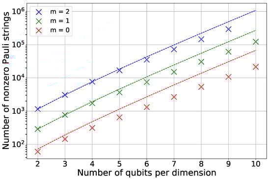
Figure 1. Number of non-zero Pauli terms in the decomposition of the Hamiltonian ${\tilde{H}}_3$ given by Equation (37). Empirical data (crosses), obtained with randomized velocity profiles for various block sizes m, are compared against the theoretical upper bound from Equation (38) (dotted line). The results demonstrate the scaling of the term count with the number of discretization qubits n for different values of m.

The empirical results reveal that the calculated upper bound closely estimates the actual count of Pauli strings. This difference arises from the distinctive configuration of the finite-difference matrix B used in our simulation. While the theoretical limit is formulated for any tridiagonal matrix, our approach uses a typical first-order stencil with matrix B having $-1$ on the main diagonal and 1 on the upper diagonal. This specific arrangement results in a more efficient Pauli decomposition, needing about $2^{n+1}$ strings for each operator, as opposed to the general maximum of $(n+1)2^{n-1}$.

The number of gates required for a single iteration of a p-th order Trotterization is based on the first-order equation as presented in Equation (26). Consequently, our analysis prioritizes the numerical validation of the first-order estimate. For the Hamiltonian ${\tilde{H}}_3$, Equation (24) provides the upper limit on the gate count for one step of a first-order Trotterization, expressed as $g_1\le \Gamma (g_d+g_z)$. Here, $\Gamma$ denotes the number of sets containing commuting Pauli strings, $g_d$ represents the gate count required to diagonalize an individual set, and $g_z$ signifies the gate count to execute the diagonal rotations in a diagonalized set.

For the block speed model, it is possible to utilize Gray code ordering within each mutually commuting set. This approach allows for further elimination of CNOT gates, thereby reducing the limit to $g_z\le 2K^{\prime }$. Previously, in Corollary 4 it was established that the block speed model restricts the number of Pauli strings per set by $K^{\prime }\le 2N{4}^m$. Thus, the limit on the number of one- and two-qubit gates for a first-order step is

$$g_1\le 3(n+1)\left[2(n+2)+4N{4}^m\right]=6(n+1)\left[n+2+2N{4}^m\right].$$

(39)

Figure 2 illustrates the results of the numerical simulation, showing how the gate counts vary with the number of qubits per dimension. We created a software program designed to produce a circuit corresponding to one Trotter step and for each collection of commuting Pauli strings. Each group’s circuit is output in QASM format for later integration into several Trotter steps. Following this, the overall gate count was ascertained from these output files. In systems where the qubit count is small, specifically $n\le 4$, we confirmed that the circuit constructed for a single group of mutually commuting operators accurately realizes $exp(-it{H}_{\gamma })$. Here, $H_{\gamma }$ represents a Hamiltonian made up exclusively of Pauli strings from that group.

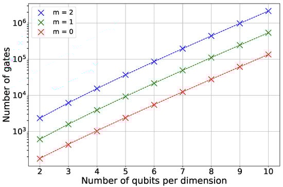
Figure 2. Gate count for a single first-order Trotter step of the Hamiltonian ${\tilde{H}}_3$. Empirical data (crosses), obtained from compiled QASM circuits, are compared against the theoretical upper bound from Equation (39) (dotted line). The results demonstrate the scaling of the gate count with the number of discretization qubits n for different velocity block sizes m.

In Figure 2, the experimental results, indicated by crosses, are slightly beneath the theoretical limit outlined in Equation (39), represented by the dotted line. This is attributed to circuit optimization techniques applied during compilation. The CNOT gates in the diagonalization circuits of each set can cancel each other out if placed in a specific order, providing a slight optimization benefit. However, the main impact comes from performing the diagonal component.

Additionally, to validate the functional correctness of the algorithm, we examined a specific instance with fixed parameters $n=5$ and $m=2$. This corresponds to solving the wave equation on a $32\times 32\times 32$ grid ($N=2^5=32$), partitioned into $2^m=4$ velocity blocks per dimension, resulting in a total of 64 individual blocks, each of size $8\times 8\times 8$ and assigned a unique velocity value. For this configuration, we verified that the implemented quantum circuit accurately approximates the action of the target unitary $exp(-i{\tilde{H}}_{3}t)$.

We assessed the accuracy by setting the initial condition to a random wavefunction $|\psi (0)⟩$ and comparing the statevector produced by our algorithm against a classical reference computed using the “scipy.sparse.linalg.expm_multiply” function in Python. Specifically, we compute the error

$$ϵ={||U(t,r,p)|\psi (0)⟩-exp(-it{\tilde{H}}_3)|\psi (0)⟩}_2||,$$

(40)

where $U(t,r,p)|\psi (0)⟩$ is the state obtained from our quantum algorithm using r Trotter steps of order p.

Figure 3 illustrates how the error varies with both the quantity of Trotter steps and the Trotter order. As anticipated, the error diminishes when the number of steps or the formula’s order is raised. This outcome confirms our implementation and offers a pragmatic calculation of the Trotter steps needed to reach a specified error threshold.

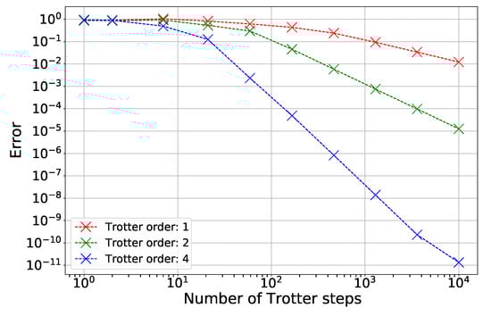
Figure 3. Trotter error scaling for the Hamiltonian ${\tilde{H}}_3$ with fixed parameters $n=5$, $m=2$. The error $ϵ$ given by (40) is plotted against the number of Trotter steps r for different Trotter orders p. The results validate the algorithm and demonstrate the expected convergence with increasing r and p.

Conducting a more thorough validation requires calculating the operator norm error ${U(t,r,p)-exp(-it{\tilde{H}}_3)}_2$ and assessing it against the bound in Corollary 4. Nevertheless, this calculation turns out to be computationally infeasible using classical methods for the matrix dimensions we are dealing with, even when n and m are relatively small.

4. Discussion

We introduced a structured quantum algorithm for simulating the multidimensional variable-coefficient wave equation. The method begins with a Hamiltonian formulation and a decomposition into Pauli strings—tensor products of $I,X,Y,Z$. This representation affords a clear physical interpretation: Z terms encode diagonal energy shifts, whereas X and Y terms generate off-diagonal transitions between basis states.

Our main contribution is a systematic extension of bounds on only relevant Pauli strings and their generation for Hamiltonians with a special block structure, together with a partition of these strings into commuting sets that admit efficient diagonalization (Propositions 1 and 2). This customizes and generalizes prior decomposition strategies [15,16] to the setting of variable-coefficient, multi-dimensional wave equations.

A second contribution is the establishment of precise gate complexity limits for calculating time evolution operators expressed as $exp(-i{\tilde{H}}_{D}t)$. Our analysis indicates that, given assumptions applicable to physical models, the gate complexity for a single Trotter step increases linearly with the size of one dimension N (Corollary 2). Nevertheless, employing Trotter–Suzuki formulas adds extra overhead: the gate complexity for the complete algorithm utilizing a p-th order Trotter formula scales as $N^{2+1/p}$ with respect to the size of a single dimension (Corollary 3). This result is significant because it tackles the challenge posed by the “curse of dimensionality”, which hinders the functionality of conventional wave equation solvers that typically scale as $N^D$ [1,2].

In contrast to oracle-based strategies [9] (with a 1D implementation in [12]), our algorithm specifies deterministic circuits in terms of one- and two-qubit gates. Although oracle-based methods may exhibit superior asymptotic query complexity, their constant factors and ancilla requirements can be substantial in regimes relevant to near-term problems [12]. Consequently, despite worse asymptotics, our explicit construction is often more practical at modest scales and enables precise resource estimation. Related oracle-dependent works [10,14] demonstrate scalability but at the cost of extra ancillas. For constant-speed models, ref [13] employs the Bell-basis approach to efficiently diagonalize each term of the Hamiltonian, yielding the same diagonalization as our method, while [11] demonstrates hardware experiments using Fourier transforms; however, these techniques do not directly extend to variable-speed profiles. In summary, relative to these lines of work, our algorithm provides explicit higher-dimensional resource bounds while accommodating variable coefficients.

For block-structured speed profiles, our analysis (Corollary 4) shows that respecting physical structure can materially reduce cost: the complexity simplifies to $2^{(D-1)m}$ when m qubits encode each block parameter (for a total of $2^{Dm}$ distinct speeds). Such piecewise-homogeneous models are common in seismic and acoustic imaging [5], making this specialization particularly relevant.

Three-dimensional simulations corroborate the predicted trends and indicate that rotation scheduling within each diagonal group can further reduce cost [21]. These optimizations are compatible with our commuting-set framework and offer practical gains without altering asymptotics.

Our use of Trotter–Suzuki decomposition entails the usual trade-off between accuracy and depth. Techniques such as qubitization [23] and linear combinations of unitaries [24] may improve asymptotic performance but generally require additional ancillas and more elaborate control logic. Moreover, our present estimates omit measurement overhead, cost-function construction, noise, and limited connectivity, all of which are consequential in the NISQ regime [25,26]. Closing these gaps is a necessary step toward end-to-end application benchmarks.

Beyond PDEs, the proposed Pauli decomposition and commuting-set diagonalization extend naturally to Hamiltonians with short-range interactions, where matrix elements cluster near the diagonal. Reducing non-commuting terms directly lowers measurement cost in variational and hybrid schemes [27,28]. The framework is also complementary to advances in randomized simulation [29], qubitization [23], and Schrödingerization [30]. We anticipate fruitful combinations that retain the structural advantages of our decomposition while improving asymptotic scaling.

Overall, the results advance quantum simulation of the wave equation in higher dimensions with variable coefficients, delivering explicit gate counts, deterministic circuit structure, and a pathway to exploiting block heterogeneity. We expect the practical advantage over oracle-based techniques observed in lower-dimensional, structured instances [15] to persist in 3D, though a like-for-like quantitative comparison remains open due to the absence of clear oracle constructions in this setting. Future work will integrate advanced simulation primitives and incorporate hardware-aware compilation and error mitigation to translate the present complexity gains into experimentally validated performance.

5. Conclusions

We have developed a general framework for quantum simulation of the multidimensional wave equation using Pauli string decomposition, diagonalization of commuting operator sets, and Trotterized time evolution. The method provides rigorous gate-complexity bounds and shows favorable scaling, particularly for the block speed model. Numerical validation in three dimensions confirms both the theoretical predictions and the potential for additional reductions through circuit-level optimization.

These results demonstrate that quantum computing can offer practical advantages for simulating high-dimensional wave dynamics, a class of problems that remain computationally demanding for classical solvers. Future directions include integrating qubitization and other advanced simulation techniques as well as designing hardware-aware circuit optimizations. The presented approach establishes a foundation for scalable quantum algorithms with applications in geophysics, nondestructive testing, and materials science.

References

- Virieux, J.; Operto, S. An overview of full-waveform inversion in exploration geophysics. Geophysics 2009, 74, WCC1–WCC26. [Google Scholar] [CrossRef]
- Taflove, A.; Hagness, S.C.; Piket-May, M. Computational electromagnetics: The finite-difference time-domain method. In The Electrical Engineering Handbook; Elsevier: Amsterdam, The Netherlands, 2005; Volume 3, p. 15. [Google Scholar]
- LeVeque, R.J. Finite Difference Methods for Ordinary and Partial Differential Equations: Steady-State and Time-Dependent Problems; Society for Industrial and Applied Mathematics (SIAM): Philadelphia, PA, USA, 2007. [Google Scholar]
- Tarantola, A. Inverse Problem Theory and Methods for Model Parameter Estimation; Society for Industrial and Applied Mathematics (SIAM): Philadelphia, PA, USA, 2005. [Google Scholar]
- Pratt, R.G. Seismic waveform inversion in the frequency domain, Part 1: Theory and verification in a physical scale model. Geophysics 1999, 64, 888–901. [Google Scholar] [CrossRef]
- Yee, K. Numerical solution of initial boundary value problems involving Maxwell’s equations in isotropic media. IEEE Trans. Antennas Propag. 1966, 14, 302–307. [Google Scholar]
- Harrow, A.W.; Hassidim, A.; Lloyd, S. Quantum algorithm for linear systems of equations. Phys. Rev. Lett. 2009, 103, 150502. [Google Scholar] [CrossRef]
- Berry, D.W. High-order quantum algorithm for solving linear differential equations. J. Phys. A Math. Theor. 2014, 47, 105301. [Google Scholar] [CrossRef]
- Costa, P.C.S.; Jordan, S.; Ostrander, A. Quantum algorithm for simulating the wave equation. Phys. Rev. A 2019, 99, 012323. [Google Scholar] [CrossRef]
- Bösch, C.; Schade, M.; Aloisi, G.; Keating, S.D.; Fichtner, A. Quantum wave simulation with sources and loss functions. Phys. Rev. Res. 2025, 7, 033225. [Google Scholar] [CrossRef]
- Wright, L.; Mc Keever, C.; First, J.T.; Johnston, R.; Tillay, J.; Chaney, S.; Rosenkranz, M.; Lubasch, M. Noisy intermediate-scale quantum simulation of the one-dimensional wave equation. Phys. Rev. Res. 2024, 6, 043169. [Google Scholar] [CrossRef]
- Suau, A.; Staffelbach, G.; Calandra, H. Practical quantum computing: Solving the wave equation using a quantum approach. ACM Trans. Quantum Comput. 2021, 2, 1–35. [Google Scholar] [CrossRef]
- Sato, Y.; Kondo, R.; Hamamura, I.; Onodera, T.; Yamamoto, N. Hamiltonian simulation for hyperbolic partial differential equations by scalable quantum circuits. Phys. Rev. Res. 2024, 6, 033246. [Google Scholar] [CrossRef]
- Sato, Y.; Tezuka, H.; Kondo, R.; Yamamoto, N. Quantum algorithm for partial differential equations of nonconservative systems with spatially varying parameters. Phys. Rev. Appl. 2025, 23, 014063. [Google Scholar] [CrossRef]
- Arseniev, B.; Guskov, D.; Sengupta, R.; Biamonte, J.; Zacharov, I. Tridiagonal matrix decomposition for Hamiltonian simulation on a quantum computer. Phys. Rev. A 2024, 109, 052629. [Google Scholar] [CrossRef]
- Arseniev, B.; Guskov, D.; Sengupta, R.; Zacharov, I. High-order schemes for solving partial differential equations on a quantum computer. Phys. Rev. A 2025, 111, 042625. [Google Scholar] [CrossRef]
- Berry, D.W.; Ahokas, G.; Cleve, R.; Sanders, B.C. Efficient quantum algorithms for simulating sparse Hamiltonians. Commun. Math. Phys. 2007, 270, 359–371. [Google Scholar] [CrossRef]
- Childs, A.M.; Su, Y.; Tran, M.C.; Wiebe, N.; Zhu, S. Theory of trotter error with commutator scaling. Phys. Rev. X 2021, 11, 011020. [Google Scholar] [CrossRef]
- Kawase, Y.; Fujii, K. Fast classical simulation of Hamiltonian dynamics by simultaneous diagonalization using Clifford transformation with parallel computation. Comput. Phys. Commun. 2023, 288, 108720. [Google Scholar] [CrossRef]
- Van Den Berg, E.; Temme, K. Circuit optimization of Hamiltonian simulation by simultaneous diagonalization of Pauli clusters. Quantum 2020, 4, 322. [Google Scholar] [CrossRef]
- Welch, J.; Greenbaum, D.; Mostame, S.; Aspuru-Guzik, A. Efficient quantum circuits for diagonal unitaries without ancillas. New J. Phys. 2014, 16, 033040. [Google Scholar] [CrossRef]
- Sato, H.; Fehler, M.C.; Maeda, T. Seismic Wave Propagation and Scattering in the Heterogeneous Earth; Springer: Berlin/Heidelberg, Germany, 2012; Volume 496. [Google Scholar]
- Low, G.H.; Chuang, I.L. Optimal Hamiltonian simulation by quantum signal processing. Phys. Rev. Lett. 2017, 118, 010501. [Google Scholar] [CrossRef]
- Berry, D.W.; Childs, A.M.; Cleve, R.; Kothari, R.; Somma, R.D. Simulating Hamiltonian dynamics with a truncated Taylor series. Phys. Rev. Lett. 2015, 114, 090502. [Google Scholar] [CrossRef]
- Kandala, A.; Temme, K.; Córcoles, A.D.; Mezzacapo, A.; Chow, J.M.; Gambetta, J.M. Error mitigation extends the computational reach of a noisy quantum processor. Nature 2019, 567, 491–495. [Google Scholar] [CrossRef]
- Preskill, J. Quantum computing in the NISQ era and beyond. Quantum 2018, 2, 79. [Google Scholar] [CrossRef]
- Cerezo, M.; Arrasmith, A.; Babbush, R.; Benjamin, S.C.; Endo, S.; Fujii, K.; McClean, J.R.; Mitarai, K.; Yuan, X.; Cincio, L.; et al. Variational quantum algorithms. Nat. Rev. Phys. 2021, 3, 625–644. [Google Scholar] [CrossRef]
- Peruzzo, A.; McClean, J.; Shadbolt, P.; Yung, M.H.; Zhou, X.Q.; Love, P.J.; Aspuru-Guzik, A.; O’brien, J.L. A variational eigenvalue solver on a photonic quantum processor. Nat. Commun. 2014, 5, 4213. [Google Scholar] [CrossRef] [PubMed]
- Childs, A.M.; Ostrander, A.; Su, Y. Faster quantum simulation by randomization. Quantum 2019, 3, 182. [Google Scholar] [CrossRef]
- Jin, S.; Liu, N.; Yu, Y. Quantum simulation of partial differential equations via Schrödingerization. Phys. Rev. Lett. 2024, 133, 230602. [Google Scholar] [CrossRef]
- Zacharov, I.; Arslanov, R.; Gunin, M.; Stefonishin, D.; Bykov, A.; Pavlov, S.; Panarin, O.; Maliutin, A.; Rykovanov, S.; Fedorov, M. “Zhores”—Petaflops supercomputer for data—Driven modeling, machine learning and artificial intelligence installed in Skolkovo Institute of Science and Technology. Open Eng. 2019, 9, 512–520. [Google Scholar] [CrossRef]
Disclaimer/Publisher’s Note: The statements, opinions and data contained in all publications are solely those of the individual author(s) and contributor(s) and not of MDPI and/or the editor(s). MDPI and/or the editor(s) disclaim responsibility for any injury to people or property resulting from any ideas, methods, instructions or products referred to in the content. |
© 2025 by the authors. Licensee MDPI, Basel, Switzerland. This article is an open access article distributed under the terms and conditions of the Creative Commons Attribution (CC BY) license (https://creativecommons.org/licenses/by/4.0/).