Abstract
Over the past several decades, there has been an accelerating trend to ever more accurate quantum sensors: sensors of time intervals (i.e., atomic clocks), sensors of magnetic fields (i.e., quantum magnetometers), and sensors of inertial motions (i.e., atom interferometers), to name just a few. With this trend has come a renewed interest in the problem of quantum mechanical measurement (i.e., collapse of the wavefunction), and though there have been many attempts to resolve the problem, there is still no wholly accepted resolution. Here, we discuss a little-explored path for resolving the issue that exploits wavefunction phase. To illustrate this path’s potential, we consider the notion of “eigenphase” sets that are disjoint among orthogonal eigenvectors. Wavefunction collapse then occurs because of constructive/destructive interference when a classical measuring device “phase-locks” to an incoming wavefunction. While the present work examines one method for exploiting wavefunction phase, its primary purpose is to more generally re-focus attention on wavefunction phase as a means for resolving the measurement problem that avoids many other solutions’ problematic aspects.
1. Introduction
Over the past several decades, there has been an accelerating trend towards the creation of quantum sensors: atomic clocks for sensing time intervals [1,2], atom interferometers for sensing non-inertial motions [3], quantum magnetometers [4], Rydberg-atom [5] and atomic candle [6,7] sensors of microwave fields, and many others. In a very real sense, “quantum engineering” is emerging as a vibrant cousin to electrical and mechanical engineering, and with this trend comes a closer scrutiny of quantum mechanical measurement as technologists question the ultimate limits and limitations of quantum sensors. Of these questions, there is no more important issue than the “measurement problem” (i.e., collapse of the wavefunction), which is receiving renewed attention in the wider physics community [8,9].
To illustrate the significance of the issue, one need only consider NASA’s Deep Space Atomic Clock [10], where an atomic superposition state created by a microwave field collapses to a hyperfine eigenstate of 199Hg+ as the ion absorbs a UV photon from an rf-discharge lamp. This device can assess the frequency of that microwave field out to the 15th significant figure and is already easily capable of sensing relativistic planetary alterations of the metric. As space-qualified atomic clocks continue to improve [11], researchers will likely need to better understand how quantum measurement plays out on a changing metric background during fly-by missions of massive astronomical objects.
The measurement problem in quantum mechanics consists principally of two parts: (1) No matter the initial wavefunction of an object, the result of a “strong” measurement [12] on that object always results in the collapse of the wavefunction into one of the eigenstates associated with the measuring apparatus. (2) Once the wavefunction collapses, it remains collapsed regardless of the object’s initial wavefunction [13]. To clarify the first issue by way of example, consider the Stern–Gerlach experiment where spin-1/2 atoms are passed through an inhomogeneous magnetic field [14,15] and assume that the apparatus is arranged to measure the atom’s spin along the z-axis of the experimental coordinate frame (i.e., the eigenstates of the measuring apparatus correspond to ∣+⟩ and ∣−⟩ relative to the z-axis). Regardless of the initial wavefunction ∣Φ⟩ of the atoms entering the apparatus (e.g., ∣Φ⟩ = a+∣+⟩ + a−∣−⟩), the result of the strong measurement will always be a manifestation of either ∣+⟩ or ∣−⟩. The measurement will never correspond to some superposition of measuring-apparatus eigenstates, even though that may have been the initial state of the object’s wavefunction.
The second part of the measurement problem states that the collapse is irreversible. In a sense, the complexity of the object is reduced by the strong measurement. Prior to the collapse, while in a superposition state, there was complexity to the object’s z-axis nature: it was partly spin-up and partly spin-down. After the collapse that complexity is lost; the atom is either all z-axis spin-up or all z-axis spin-down.
The reason that quantum-state measurement is often viewed as problematic has to do with the “schizophrenic” split (to quote from DeWitt [16]) that it creates in the foundational nature of change in quantum mechanics. On the one hand, in the absence of measurement, a wavefunction evolves in time under the action of a Hamiltonian in a deterministic manner: von Neumann’s T2 process [17]. However, when a strong measurement takes place, the wavefunction evolves discontinuously; it evolves in an irreversible manner, and its evolution is probabilistic as opposed to deterministic with probabilities given by the Born rule [18]: von Neumann’s T1 process [17]. How one resolves these two quite distinct natures of change into a coherent whole has been a foundational problem in quantum mechanics since its beginning [19], and the success or failure of various attempts to solve the problem is still largely a matter of opinion.
In this paper, we want to revisit a solution pathway to the measurement problem first touched on by Bohm [20] and then more carefully pointed out by Pearle [21]. Bohm noted that every measurement involves an interaction, and that through the interaction the combined quantum-entity/measuring-device wavefunction develops a random phase. On average, this random phase keeps measuring-device “pointer states” solely associated with their corresponding quantum-particle eigenstates. Unfortunately, in Bohm’s analysis, these random phases do nothing to resolve the problem of wavefunction collapse. Pearle took the phase idea a bit further, arguing that if the phase of a wavefunction were a random variable, then along with a nonlinear Schrödinger equation this random phase would lead to wavefunction collapse. Here, we also focus on wavefunction phase as central to the measurement problem. However, different from Pearle, we take quantum mechanics as linear.
Prior to discussing our wavefunction-phase pathway, we present in the next section a very brief review of some of the present leading candidates for solving the measurement problem, considering their advantages as well as their problematic aspects. We then turn to some preliminary issues: the notion of global phase in textbook quantum mechanics and the very general concept of measurement itself. Following these preliminaries, we discuss one wavefunction-phase pathway as a concrete illustration of the pathway’s broader potential for resolution of the measurement problem and its ability to circumvent other solutions’ problematic aspects.
2. Some Attempts to Solve the Measurement Problem
2.1. Copenhagen Interpretation
The standard solution to the measurement problem routinely found in textbooks follows from the Copenhagen Interpretation of quantum mechanics. Briefly, the wavefunction is interpreted solely as a computational device that provides probabilities for the results of experimental outcomes; it is not indicative of a quantum entity’s actual nature [22]. When a measurement occurs, new information regarding the quantum entity is obtained. In the Copenhagen Interpretation, the wavefunction does not really collapse during a strong measurement. Rather, measurement provides new information regarding the quantum entity, and consequently the tool for predicting further experimental outcomes (i.e., the wavefunction) must be updated. Thus, in the Copenhagen Interpretation, there is no measurement problem. What we call collapse of the wavefunction is nothing more than the manifestation of one of the entity’s stochastic potentialities and an updating of the tool for future computation. (To be clear, the Copenhagen Interpretation does not imply that the quantum object has some well-defined eigenstate prior to measurement; rather, in the Copenhagen Interpretation, it is meaningless to talk about the state of a quantum object prior to measurement, since, by definition, no measurement has taken place to determine the object’s state.)
Though pragmatic in the sense that the Copenhagen Interpretation allows the practicing physicist to proceed with their use of quantum mechanics without worry of foundational issues, it does nonetheless have detractors. Many practicing physicists would likely rebel against the view of the wavefunction as nothing more than a computational tool. They would likely see the wavefunction as an actual reflection of a quantum entity’s nature. Some might even argue that they do in fact “touch” the wavefunction through (for example) atom interferometry experiments [23,24] and weak measurements [25].
2.2. Many Worlds Interpretation
Another solution to the measurement problem originated with Everett as the Many Worlds Interpretation of quantum mechanics [26]. In this interpretation, the total wavefunction of the object/observer (i.e., object/measuring-device) system is viewed as an entangled superposition state of object eigenvectors and their corresponding measurement-device eigenvectors. It is not that the object’s wavefunction collapses, but rather that each of the object/observer potentialities is realized, with each realization manifesting itself as a splitting of the universe into a set of disconnected branches. There is one observer for each branch of the splitting, and that observer measures one specific manifestation of the quantum object’s multitude of potentialities.
As with the Copenhagen solution, the Many Worlds solution to the measurement problem has its supporters and detractors. On the one hand, it neatly avoids the dualism of von Neumann’s T1 and T2 processes: there are only T2 processes, and the appearance of T1 processes is an artifact of an observer confined to one branch of a multiverse. However, for many, this requires the uncomfortable acceptance of a multiverse, with branches rapidly multiplying and forever isolated from one another.
2.3. Decoherence Theory
In recent years, attention has been directed towards the Decoherence Theory of measurement [27]. In any measurement of a quantum entity by a laboratory measuring apparatus, we are dealing with a macroscopic device that is, at heart, an open quantum system coupled to the environment. Thus, as the quantum entity interacts with the measuring device, the near-infinite degrees of freedom the environment brings into the problem result in a very rapid loss of coherence among linearly superposed eigenvectors in the entity’s wavefunction. Consequently, the density matrix describing a sequence of measurements on the quantum entity is always diagonal; there is zero probability of having a measurement that represents a superposition of eigenvectors. Thus, in Decoherence Theory, collapse of the wavefunction is an observational consequence of measuring quantum entities with macroscopic devices coupled to the environment.
Again, as with the other solutions to the measurement problem, Decoherence Theory has its adherents and detractors. On the one hand, it recognizes that ideal measurements, isolated from the world around them, exist primarily in the physicist’s imagination. Actual measurements with real measuring devices always have some coupling to the world at large, and, in Decoherence Theory, that coupling plays a central role in what can and cannot be observed and measured. Critics, of course, could argue that Decoherence Theory only “sweeps the measurement problem under the rug,” since it relies on a general very rapid loss of coherence that by rights should be clearly articulated and defined in every measurement situation. Further, critics could reasonably argue that if one could decouple a macroscopic measuring device from the environment at large, then one could find the measuring device in a superposition of measuring-apparatus eigenstates. One might also argue that Decoherence Theory creates an epistemological problem for quantum mechanics, since it is only the density matrix that reflects experimental outcomes. Consequently, it can be argued that it forces the physicist to accept the density matrix’s Liouville equation as more foundational than the Schrödinger equation.
2.4. Spontaneous Collapse Models
Spontaneous Collapse Models start from the assumption (even if not specifically articulated) that there is some random field permeating the universe, which cannot be a standard quantum field. This field couples to “quantum matter through an anti-Hermitian and nonlinear coupling” [28]. At random times, this coupling causes the wavefunction to localize and thereby results in the collapse of the wavefunction into one of its eigenstates.
Though logically consistent, and amenable to experimental investigation, many would argue that the requirement for a nonlinear Schrödinger equation is at a minimum distasteful. Furthermore, requiring a non-quantum field that permeates all of space, likely with a cosmological origin, opens a host of new problems related to the structure and evolution of the universe.
2.5. General Character of Solutions to the Measurement Problem
In each of these potential measurement problem solution cases, the solution should be seen as having a dyadic nature. For one part of the solution, there is a statement regarding textbook quantum mechanics: either textbook quantum mechanics requires modification, or it does not. For the second part, there is a measuring “protocol” statement. For example, in the Many Worlds interpretation, there is no specific change to textbook quantum mechanics, but there is a measuring protocol statement regarding the introduction of an unknowable multiverse. In Spontaneous Collapse Models, nonlinearity is introduced into textbook quantum mechanics, while the measurement protocol hypothesizes the operation of a quantum-entity/non-quantum-field interaction. In Decoherence Theory, textbook quantum mechanics is taken without modification, and the measuring protocol is the interaction of a heat-bath with the coupled quantum-entity/measuring-device system. Even in the Copenhagen Interpretation, there is what amounts to an epistemological protocol: “one cannot know without measurement; therefore, it is meaningless to talk about a quantum entity existing in a superposition or entangled state.”
2.6. Overview of Wavefunction Phase as a Path to Resolution of the Measurement Problem
There are, of course, many other suggested solutions to the measurement problem [29,30] with some of these distinct from those mentioned above and some novel modifications [31,32,33,34,35]. Here, we want to re-open discussion of a path to resolution of the measurement problem that avoids many of the issues listed in the preceding and follows from ideas touched on by Bohm [20] and introduced by Pearle [21]: a wavefunction-phase path.
To demonstrate the potential of this pathway, we focus on the global phase invariance of operator eigenvectors. Rather than taking global phase invariance as continuous (modulo two pi), we allow each eigenvector to have a set of unique phases (of extremely large cardinality) with the sets disjoint between eigenvectors: no phase appearing in one set equals the phase appearing in an orthogonal eigenvector’s phase set. This does not destroy the U(1) symmetry of the eigenvectors since all measurements remain invariant with respect to a U(1) transformation of the wavefunction.
Similar to other solutions to the measurement problem, we introduce a measurement protocol: during the measurement process, the classical measuring device “phase-locks” to the incoming quantum particle. With this slight change to textbook quantum mechanics (eigenphase sets) and the measurement protocol (quantum-particle/measuring-device phase-locking), wavefunction collapse occurs as a consequence of constructive/destructive interference between the macroscopic measuring device and the quantum particle.
Advantages to this solution pathway are several. Contrary to the Copenhagen Interpretation, the wavefunction is seen as an object that describes the actual nature of a quantum object, and in addition the wavefunction-phase solution does not require postulating a rapidly expanding multiverse. The wavefunction-phase pathway also gives primacy to the Schrödinger equation, which is (arguably) different from Decoherence Theory. Importantly, the wavefunction-phase pathway to resolution of the measurement problem takes quantum mechanics as linear, which all experiments to date support. There is no nonlinear aspect to the fundamental equations of Nature, nor is there a need for a cosmological random field that couples to matter as in Spontaneous Collapse Models.
We also note that the wavefunction-phase pathway is not a Hidden Variables Theory [36] as will be partially demonstrated subsequently. A wavefunction’s global phase is a fundamental element of standard quantum theory. It is in no way an extra parameter added into quantum mechanics and manifests itself in countless atomic interference experiments (e.g., atomic clocks and atom interferometers). An excellent experimental/technological example of this is provided by atomic clocks based on Coherent Population Trapping (CPT) [37]. With CPT, two routes of optical excitation within an atom are simultaneously excited. However, since the two routes (i.e., matrix elements) have different phases, they destructively interfere, which results in no optical absorption though both optical excitation routes are resonantly excited.
3. Some Preliminary Considerations
3.1. Wavefunction Phase in Standard Quantum Mechanics
It is well known that the solution of the Schrödinger equation is not unique. There are an infinite number of solutions, distinguished from one another by a global phase. Specifically, if Φeiα is a solution to the Schrödinger equation (with α a constant), then so is Φeiβ with α ≠ β. This is to be distinguished from the fact that the evolution of every quantum entity plays out in spacetime, which gives the wavefunction a spacetime dependence. Specifically, with every wavefunction, there is typically a phase factor of the form , where the xμ are spacetime coordinates. It is worth noting , where xoμ is routinely taken as the origin of an arbitrarily defined coordinate system. As such, xoμ is one manifestation of a wavefunction’s global phase.
All of this is routinely illustrated in quantum textbooks through the example of a free particle’s wavefunction:
where we have explicitly included the global phase α. In many experiments and quantum devices, the kμxμ phase factor plays an important role, such as in atomic clocks where it leads to Ramsey’s separated oscillatory fields method for atomic signal generation [38,39]. However, in these devices and experiments, the global phase factor eiα plays no role.
As a textbook illustration of the usual irrelevance of the global phase factor, consider a perturbation V that causes transitions between the eigenstates of a Hamiltonian. The transition rate between the initial state ∣i⟩ and the final state ∣f⟩, Γif, is given by Fermi’s Golden Rule:
where ρ(Ef) is the density of final states. If we allow these two orthogonal eigenvectors to have different phases: αi and βf, Equation (2) becomes
The global phase factor has dropped out of the transition probability.
The same will be true for collision cross-sections or any other observable. Consequently, in computations, it is routine to set the global phase factor of an eigenvector to zero. With regard to present considerations, all of this illustrates the tremendous freedom within standard quantum mechanics regarding an eigenvector’s global phase. No matter how one chooses to define a wavefunction’s global phase, the results of textbook quantum mechanics are unaltered.
3.2. Measurement
As discussed more fully in Appendix A, a measurement is very generally a mapping from the entity to be measured (i.e., the measurand) to a categorical manifestation of the measured entity (often quantifiable). In other words, we can define the measuring process through a mapping operator that projects the measurand’s state onto a measuring-device “response state.” Of course, for a strong quantum measurement [25], which is the only type we consider here, the mapping irreversibly couples the measurand and measuring device. In other words, the wavefunction of the measurand collapses.
It is also important to note that physical measurement processes are one-to-one: one quantum entity gives rise to one measuring-device response. For example, in the detection of a single photon, conservation of energy requires the generation of one photodiode current-pulse equivalent to the photon’s energy (independent of any measuring-device gain). In the destructive detection of a single charge-carrying particle, conservation of charge requires the measuring device to create one charge-equivalent response (again prior to any measuring-device gain).
Here, we capture this notion of measurement through a mapping operator M that projects the combined initial state of the quantum wavefunction and measuring device to some final state. To keep the discussion focused, we restrict our considerations to a two-state quantum entity interacting with a three-state measuring device. The quantum measurand can therefore be in the “down” state ∣−⟩ or the “up” state ∣+⟩, or it can be in some down/up superposition state. (We can also think in terms of a photon’s polarization, with the down state corresponding to horizontal polarization and the up state to vertical polarization.) The measuring device can be in the neutral state ∣m0⟩ (e.g., producing no measurement response), the down measurement response state ∣m−1⟩, or the up measurement response state ∣m+1⟩; for each of these measurement response states, there is a unit-valued, measurement pointer: Aq, which is the measuring device’s output for a single quantum-measurand detection. Thus, we write M as
Note that similar to Decoherence Theory [27] and Bohm’s analysis of measurement [20], there is no phase coherence among the measuring-device’s response states (i.e., the off-diagonal elements are zero). This is consistent with the coupling of a classical, macroscopic measuring device to an environmental heat-bath. Of course, loss of phase coherence among the measuring-device’s response states can also occur via incoherent coupling of the quantum entities making up the measuring device to one another (e.g., the individual atoms or domains making up a classical magnet).
As an example of this measuring operator’s application, consider the incoming wavefunction in a superposition state:
The initial state of the measurand/measuring device is ∣Φ⟩∣m0⟩, so that the mapping operator acting on this wavefunction yields
The measurement process has entangled measuring-device response states and quantum-entity eigenstates. Thus, taking the norm of this final measurand/measuring-device state (i.e., ∣Ψ⟩ = M∣Φ⟩∣m0⟩) as the output of the measuring-device, we have
The output of the measuring device can be either A+1 or A−1 with probabilities ∣a+∣2 and ∣a−∣2, respectively.
Given this result, it would appear that we have done nothing with the measurement operator of Equation (4) but arrive back at the measurement problem (i.e., no collapse of the wavefunction within standard quantum mechanics). However, that is precisely the point. There is nothing novel in writing Equation (4); it is fully consistent with standard quantum mechanics [20]. As we will show in the following sections, by positing disjoint eigenvector phase sets, the entanglement of Equation (7) is eliminated, with the result that the measuring device produces either A+1 or A−1 but not both.
4. Eigenphase Sets and Measurement
4.1. Overview
As previously stated, there is considerable freedom within standard quantum mechanics in setting an eigenvector’s global phase. We can take advantage of this freedom by postulating an addition to textbook quantum mechanics, which in no way violates the tenants of standard quantum mechanics. To each eigenvector of an Hermitian operator (e.g., angular momentum), we assign a set of unique “eigenphases” (which we take as distributed uniformly between −π and π radians for convenience), and define these sets as disjoint for orthogonal eigenvectors. Consequently, no matter where or when an eigenvector manifests itself, the global phase of that eigenvector will always be drawn from its unique set of eigenphases.
In the present case, for an operator with two eigenvectors, ∣+⟩ and ∣−⟩, there will be two eigenphase sets: {θ} and {ϕ}. Specifically, ∣+⟩eiθ1, ∣+⟩eiθ2,… ∣+⟩eiθN are all equivalent ∣+⟩ eigenvectors, while ∣−⟩eiϕ1, ∣−⟩eiϕ2,… ∣−⟩eiϕN are all equivalent ∣−⟩ eigenvectors; for all i and j, θi ≠ ϕj. Note that while the cardinality of the eigenphase sets will be very large (e.g., 1017), every manifestation of an eigenvector is nonetheless a single ray in Hilbert space.
Clearly, a significant caveat to this assumption is that the phase sets contain a finite number Nφ of elements. Though we speculate on possible origins for the eigenphase sets’ finite size in Appendix D, here we simply note that the value of Nφ will be exceedingly large. Consequently, Δφ ~ 2π/Nφ is so small that, in any experiment sensitive to an eigenvector’s phase (e.g., atom interferometry), the global phases within a set would have the appearance of continuity and no measurable influence on experimental outcomes.
With this modification to textbook quantum mechanics comes the issue of a solution to the Schrödinger equation when the Hamiltonian and operator of interest (e.g., Sz) do not commute, such that in expressing the Schrödinger equation’s solution ∣Φ⟩ in terms of the operator-of-interest’s eigenvectors, we have essentially two choices regarding the global phase, namely
or
The problem with Equation (8a) is readily apparent: for any general Hermitian operator O, the expectation value of the operator would become a random variable depending on how the disjoint global eigenphases θ and ϕ manifest:
In other words, with Equation (8a), the matrix elements of a Hermitian operator become random variables, which is clearly not borne out by experiment. Thus, the only way to write a superposition state consistent with experience is Equation (8b).
To relate the phase η to the sets of eigenphases {θ} and {ϕ}, we note from Born’s rule [18] that ∣a+∣2 and ∣a−∣2 are the probabilities for finding the state ∣Φ⟩ in either ∣+⟩ or ∣−⟩, respectively. Thus, it should be that
where P[η = {X}] is the probability that η takes on one of the values in the set {X}. Consequently, from the perspective of eigenphases, Born’s rule is not so much an “added on” statement regarding experimental outcomes, but rather a quantum rule assigning the probability for choosing a superposition wavefunction’s phase from one of the possible eigenphase sets.
It is also important to note that this modification of textbook quantum mechanics has no effect on expectation values. Given any Hermitian operator O and considering the wavefunction of Equation (8b),
which is independent of any stochastic nature to the wavefunction’s phase. Moreover, Equation (8b) maintains the U(1) transformation invariance of inner products involving eigenvectors. Recognizing that the U(1) transformation (i.e., eiα) is independent of the global phase choice, U(1)∣Φ⟩ = [a+∣+⟩ + a−∣−⟩]ei(η+α) ⟹ U(1) [⟨Φ∣O∣Φ⟩] = ⟨Φ∣O∣Φ⟩.
4.2. The Measurement Operator and Eigenphase Sets
To incorporate the concept of eigenphase sets into the measurement operator, we now rewrite Equation (4) as
In this expression, the global phase terms in the two summations capture interference between the incoming quantum measurand and the multitude of quantum objects making up the classical, macroscopic measuring device, each with its own global eigenphase. Further, since the macroscopic measuring device is obviously constructed from an Avogadro’s number of quantum entities, all interacting with the quantum measurand, the classical measuring device presents the complete set of eigenphase values to the incoming quantum measurand. This is appropriate so long as the number of quantum entities in the measuring device, Nm, is significantly greater than Nφ. (Thoughts on the Nm/Nφ ratio are discussed in Appendix D.) Finally, g±1 captures the fact that for a single measurement with Nm measuring-device quantum objects, the result of the measurement must nonetheless be one-to-one: one quantum measurand produces one measuring-device response. Note that if all the eigenphases were zero, and the g±1 were equal to unity, then Equation (12) would reduce to Equation (4).
4.3. Quantum-Measurand and Measuring-Device Phase-Locking
As already noted, in all present solutions to the measurement problem, there is a protocol that leads to wavefunction collapse. To re-iterate,
- In the case of the Copenhagen interpretation of quantum mechanics the protocol is an appeal to epistemology. Specifically, since one cannot know without measurement; it is pointless to consider the state of the wavefunction prior to measurement. While theory may allow one to write the state of the wavefunction as a superposition of eigenvectors prior to measurement, this mathematical statement is solely a convenient way of capturing how an experiment might turn out. It is in no way a description of reality, since reality cannot be known without measurement. Clearly, there is no possibility of experimentally testing this protocol since the appeal to epistemology effectively redefines the measurement problem away.
- In the Many Worlds hypothesis, the protocol is an appeal to a multiverse. There is no collapse of the wavefunction, each possible result of a measurement is in fact realized. Since observers are confined to one particular universe within the multiverse, an observer experiences only one of the myriad results that are obtained from measurement. In fact, however, all possible results are obtained. Again, there is no way of experimentally testing this protocol, since each universe in the multiverse is forever cut-off from all others. One must take it “on faith” that the multiverse exists.
- The protocol of Decoherence Theory clearly has an intuitive appeal, since it focuses on the coupling of a real measuring device to its laboratory environment. Through this coupling, off-diagonal elements of the density matrix rapidly decay to zero, so that experimental outcomes must devolve to the diagonal elements of the density matrix, which describes the probability of finding the wavefunction in one eigenvector or another. Nevertheless, the protocol does lead to a provocative (and some might say disturbing) thought experiment. If one could manage to decouple a classical measuring device from the environment, would (for example) a Stern–Gerlach apparatus lead to the detection of a spin-up/spin-down superposition state?
- Finally, the protocol of Spontaneous Collapse Models is an appeal to a random (non-quantum) field pervading the universe and, while controversial, does have the advantage of possible experimental verification [40]. Nevertheless, we note again (as with all other solutions to the measurement problem) that Spontaneous Collapse Models require a measurement protocol to achieve wavefunction collapse.
Here, our measurement protocol involves a classical measuring device “phase-locking” to an incoming quantum measurand. Prior to obtaining the measurement output, the measuring operator transitions via this phase-locking: M ⟶ TPL[M], where TPL indicates the phase-locking transformation of the measuring device.
As discussed in Appendix B, depending on the phase of the measurand’s wavefunction, two possibilities present themselves for phase-locking:
- (1)
- If η is an element of the set {θ}, then all terms in the top left sum of Equation (12), except for η = θK (i.e., the actual phase of the incoming wavefunction) have (η − θJ) = π, and all terms in the lower right sum have (η − ϕJ) = π.
- (2)
- If η is an element of the set {ϕ}, then all terms in the lower right sum of Equation (12), except η = ϕK (again the actual phase of the incoming wavefunction), have (η − ϕJ) = π, and all terms in the top left sum have (η − θJ) = π.
Consequently, after phase-locking, the sums in Equation (12) reduce to a series of Kronecker deltas:
In effect, the incoming quantum measurand and phase-locked measuring device have destructively interfered for all eigenphases other than η.
To examine this measurement process concretely, we apply TPL[M] to the superposition state of Equation (8b), considering (for illustrative purposes) the specific case of η = θK: the phase of the incoming quantum-state measurand for this one particular realization of the quantum entity comes from the set of unique eigenphases associated with the ∣+⟩ eigenvector. Applying TPL[M] to this incoming quantum measurand then yields the measurand/measuring-device combined state after measurement, ∣Ψ⟩:
It should be noted that ∣Ψ⟩ is not a state in the usual quantum sense, since it is a mixture of a quantum state and a classical measuring-device response-state (i.e., ∣m+⟩) as it must be. Consequently, the norm of ∣Ψ⟩ is not unity but rather the magnitude of the classical measuring device’s output A±1.
The value of g±1 in Equation (14) is fixed by the requirement that the measurement be one-to-one:
yielding
Interestingly, for the classical measuring device to always produce a one-to-one response, regardless of the value of a+, the classical measuring device must in effect increase its sensitivity to an eigenvector as that eigenvector’s contribution to the overall measurand wavefunction decreases. Given Equation (16), we arrive at
The measuring device is in the single response-state ∣m+⟩ with norm A+1, and the quantum-measurand wavefunction has collapsed to ∣+⟩eiθK with unit norm.
If the measurement process leading to Equation (17) is repeated many times, then different results will be obtained depending on the values of the quantum-measurand’s phase. The probability of finding the macroscopic measuring device in the state ∣m+⟩ and obtaining the quantity A+1 for the measurement’s manifestation will be equal to the probability of having the quantum-measurand’s phase η equal to a member of the eigenphase set {θ}, which is just ∣a+∣2. Similarly, the probability of finding the macroscopic measuring device in the state ∣m−⟩ and obtaining the measurement manifestation A−1 will be equal to the probability of η = {ϕ}, which is just ∣a−∣2. Consequently, the statistics of measurement outcomes is consistent with the Born rule. Moreover, as seen here, the Born rule is not an after-the-fact addition to quantum mechanics for the prediction of experimental outcomes. Rather, the Born rule follows from the probability that a wavefunction’s phase is drawn from one or another eigenphase set.
5. Hidden Variables and Eigenphase Wavefunctions
5.1. Eigenphase Sets and Bell’s Inequality
As is well known, modifications to quantum mechanics involving hidden variables are inconsistent with experiment, and so it is reasonable to ask if the present use of eigenphase sets does not somehow correspond to a hidden-variables solution to the measurement problem. To demonstrate that this is not the case (at least partially), it will be useful to show that quantum mechanics with eigenphase sets yields the exact same results for a Bell’s inequality experiment as standard quantum mechanics without eigenphase sets. Saying this differently, if the inclusion of eigenphase sets to standard quantum mechanics (QM) was a Local Hidden Variables Theory (LHVT), it must necessarily lead to different results for a Bell’s inequality experiment.
To investigate the question, we first consider the typical Bell’s inequality experiment as shown in Figure 1, from the viewpoint of standard quantum mechanics. In this case, two spin-1/2 particles are in a singlet entangled state ∣Φ⟩ given by
One of the particles in the entangled state is sent towards the a-detector system, while the other is sent towards the b-detector system. Further, we will assume that the a-detector is set to measure particles in a rotated basis set:
Similarly, the b-detector is set to measure particles in an oppositely rotated basis set with a different rotation angle:
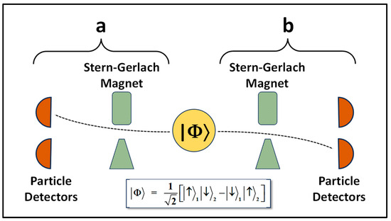
Figure 1.
Typical Bell’s inequality experiment for a spin-1/2 entangled system.
The probability of detecting a spin-up signal in the a-detector system, while simultaneously detecting a spin-down signal in the b-detector system (i.e., Pa↑,b↓) is
Substituting from Equations (18), (19a) and (20b), we then have
and working through the multiplications and trigonometry we find that
This is the Bell’s inequality experimental result that is predicted from standard quantum mechanics, and which is inconsistent with any Local Hidden Variables Theory. (See the discussion in Ref. [41].)
Considering now quantum mechanics with eigenphase sets, let {θ} be that set of eigenphases associated with ∣↑⟩ and {ϕ} be the set of eigenphases associated with ∣↓⟩; Equation (18) then becomes
Here, θ1 and ϕ2 are particular random choices out of the sets {θ} and {ϕ} for particle-1 and particle-2, respectively, and we have written the phase term consistent with Equation (8b), recognizing that the entangled wavefunction is a combination of product states with each term in the product state bringing with it a global phase. Clearly, for some other realization of the entangled wavefunction, we could have ϕ1 and θ2, namely particle-1’s phase drawn from the set {ϕ} and particle-2’s phase drawn from the set {θ}. Note also that because Equation (24) refers to a singlet state, the phase factor consists of one phase from the set {θ} and one phase from the set {ϕ}. If we had considered a triplet state, then the phase factor could have consisted of two phases from the set {θ} or two phases from the set {ϕ}.
Using Equation (24) along with Equations (19a) and (20b), we obtain for Pa↑,b↓
or taking the ei(θ1+ϕ2) phase factor out of the absolute value
But this is just Equation (22), yielding
The identity of Equation (26) with Equation (23) shows that including eigenphase sets in standard quantum mechanics leads to the same result as textbook quantum mechanics for a Bell’s inequality experiment. Therefore, including eigenphase sets into quantum mechanics cannot be a Local Hidden Variables Theory. Moreover, to try and state that wavefunction phase is somehow a hidden variable would be inconsistent with standard quantum mechanics where eigenvectors exist in a complex Hilbert space: ∣Φ⟩ = abs[∣Φ⟩]eiψ. In the next subsection, we consider how wavefunction collapse occurs in the Bell’s inequality experiment with the inclusion of eigenphases.
5.2. Collapse of the Wavefunction in a Bell’s Inequality Experiment
To elucidate the nature of wavefunction collapse in a Bell’s inequality experiment using eigenphase sets, we consider the simplified experimental situation where α = β = 0 in Equations (19) and (20). Further, we should recognize that both the ‘a’ and ‘b’ measuring devices of Figure 1 will have their own measurement operators, M(a) and M(b), and that these will only respond to those components of the entangled wavefunction reaching them. For conceptual concreteness, we will imagine that Equation (24) describes an HD molecule in its singlet ground state (i.e., a hydrogen-deuterium molecule), and that for the Bell’s inequality experiment we are “gently” stretching the molecule, adding kinetic energy to the molecular bond.
Again, this is only one realization of the molecular wavefunction, and in some other realization, we could have θH ⟶ ϕH and ϕD ⟶ θD.
For clarity in this gedanken experiment, we will also imagine that the system in Figure 1 is modified by adding a “mass-filter” prior to each Stern–Gerlach magnet. If we consider that the HD stretching energy is equally partitioned between the H and D atoms, then the separation velocity of these two must necessarily be different by the ratio (mH/mD)1/2. Knowing this, we could place the deuterium detector (e.g., the b-detector) closer to the HD source and restrict our measurement results to coincidental counts from the two detector systems. If a deuterium atom is emitted towards the b-detector, then the spin measurements of the ‘a’ and ‘b’ detectors will be coincident. If a hydrogen atom is emitted towards the b-detector, then the b-detector’s spin measurement will precede the ‘a’ detector’s measurement. Note that this mass filter does not alter the spin entanglement. Rather, it simply reduces the number of spin measurements in the Bell’s inequality experiment. Consequently, we will consider the b-detector system as examining only the spin of the deuterium atom and the a-detector only measuring the spin of the hydrogen atom. Note that this does nothing to the entangled nature of the spins; it simply reduces the Bell measurement results by one half, since any time a hydrogen atom is stretched towards the b-detector, that measurement will not be included in the Bell’s inequality results.
To proceed, with the H-atom traveling towards the a-detector and the D-atom traveling towards the b-detector, Equation (13) becomes
As a result, each measuring device phase-locks to either the H-atom’s eigenphase or the D-atom’s eigenphase, and after phase-locking, the result of this one particular ‘a’ and ‘b’ detector measurement yields
Detector ‘a’ collapses the entangled spins into a spin-up state for the H-atom, while the b-detector collapses the entangled spins into a spin-down state for the D-atom. Though we only considered the simplified case of α = β = 0, nothing precludes the analysis from recreating the situation of α ≠ β ≠ 0 discussed previously.
6. The Uncertainty Principle and Eigenphase Sets
To be fully consistent with quantum mechanics, the use of a wavefunction’s global phase to resolve the measurement problem must be consistent with the uncertainty principle, which is arguably the foundation upon which all of quantum mechanics is built. As discussed in a number of textbooks [42,43], for two Hermitian operators A and B, the uncertainty principle follows from their commutator:
where ∣Φ⟩ is the state of the particle in which the eigenvalues of A and B are obtained. Here, ΔA is the uncertainty in the measured eigenvalue of A, which is defined as ∣(A − ⟨A⟩I)Φ∣ with a similar definition for ΔB.
To demonstrate that global phase is consistent with the uncertainty principle, we again consider the uncertainty for A and B measurements of a two-state particle in a superposition state as given by Equation (8b):
Using Equation (31) to determine ΔA (and similarly ΔB), we have
and we see that the global phase has dropped out as a consequence of the absolute value in the definition of ΔA. For the right-hand-side of Equation (30), we obtain
and again the global phase has dropped out. Thus, the uncertainty principle is transparent to eigenphase sets, because (1) each particle’s phase is global and unaffected by the action of any Hermitian operator (i.e., Equation (32b)) and (2) because the definition of uncertainty is in terms of an eigenvalue’s magnitude (i.e., Equation (32a)).
7. Summary
In this work, we focused on one possible pathway for a wavefunction-phase resolution of the measurement problem with the goal of highlighting the broader potential of such a pathway. Here, we considered a modification to textbook quantum mechanics and a protocol regarding the interaction between a single quantum entity and a classical, macroscopic measuring device:
- Modification—To each eigenvector of an Hermitian operator, there is a set of discrete eigenphases, with orthogonal eigenvectors having disjoint eigenphase sets.
- Protocol—A classical, macroscopic measuring device phase-locks to the global phase of an incoming wavefunction.
Though a number of ideas regarding resolution of the measurement problem are under active debate, there are several advantages to the wavefunction-phase pathway that should be noted:
- (1)
- There is no need to define the wavefunction as solely a computational device, which is not indicative of a quantum entity’s actual nature—Copenhagen Interpretation.
- (2)
- There is no need to postulate a rapidly expanding multiverse—Many Worlds Theory. Here, wavefunction collapse is a consequence of destructive interference between a phase-locked macroscopic object and a single quantum-entity measurand.
- (3)
- There is no need to hypothesize the existence of a non-quantum random field pervading the Universe—Spontaneous Collapse Models. Stochasticity arises from a wavefunction’s random “choice” of global phase.
- (4)
- There is no epistemological problem for quantum mechanics. The Schrödinger equation is more foundational than the density matrix’s Liouville equation—Decoherence Theory.
- (5)
- There is no need to hypothesize a fundamental nonlinear theory of nature to which standard quantum mechanics is an approximation. Quantum mechanics is fundamental, and if nonlinearity enters the measurement problem at all, it is through the interface between the quantum and classical regimes (e.g., a classical measuring device’s phase-locking process).
- (6)
- There is no schizophrenic split between von Neumann’s T1 and T2 processes. Quantum mechanics solely involves T2 processes. Apparent T1 processes arise from destructive interference between a measuring device and a quantum measurand.
All of this is not to say that the use of a wavefunction’s global phase to resolve the measurement problem has no outstanding questions requiring further study.
- Is it indeed true that a macroscopic object can phase-lock to a single quantum entity, and are there experiments that might test this? Though this is a question future work will hopefully address, we present some preliminary thoughts on how phase-locking might occur and be tested in Appendix C.
- How might discretization of a wavefunction’s global phase arise? We present some conjectures in Appendix D arguing that the concept of eigenphase sets with very large cardinality is viable.
Regardless of the questions noted above, what we have really demonstrated in this work is the potential of a little-explored path for resolving the measurement problem. It is our contention that this pathway has much to recommend it and should be studied further and critically discussed.
Funding
This work was funded by the U.S. Space Force Space Systems Command under Contract No. FA8802-19-C-0001.
Data Availability Statement
The original contributions presented in the study are included in the article, further inquiries can be directed to the corresponding author.
Conflicts of Interest
Author was employed by the company The Aerospace Corporation. The author declares that the research was conducted in the absence of any commercial or financial relationships that could be construed as a potential conflict of interest.
Appendix A. Measurement
In any attack on the measurement problem, one must first define the meaning of measurement. Superficially, of course, the meaning of “measurement” seems self-evident, and many physicists (including Einstein [44]) have expressed their concept of the measurement process. However, before too quickly accepting these physics-focused definitions, we should recognize that many scientific disciplines beyond physics have grown in their measurement capabilities [45,46,47], and with this growth has come a broader understanding of scientific measurement and its relation to the objective world [48]. Consequently, since the measurement problem is longstanding, it would seem prudent to consider what measurement means for the broader scientific community.
According to the International Vocabulary of Metrology [49], measurement is defined as a “process of experimentally obtaining one or more quantity values that can reasonably be attributed to a quantity,” with measurand defined as the “quantity intended to be measured.” Measurement method is a “generic description of a logical organization of operations used in a measurement,” and the measurement result is the “set of quantity values being attributed to a measurand together with any other available relevant information.”
Of course, it can be argued that even as general as these definitions appear, they are nonetheless too limited, focusing as they do on the concept of quantity. Some argue that there are objects of measurement that do not so easily lend themselves to quantity but are nonetheless measurands. In physics, one could reasonably argue that particle spin is an example of such a measurand. Though a particle with spin may possess a magnetic moment that is related to its spin, and which can be measured as a quantity, spin itself is an angular momentum generator of rotations, which is often best described as categorically “up” or categorically “down.”
Ferris has argued for a more encompassing definition of measurement [50]: “Measurement is an empirical process, using an instrument, effecting a rigorous and objective mapping of an observable into a category in a model of the observable that meaningfully distinguishes the manifestation from other possible and distinguishable manifestations.” Here, the operative idea is a mapping between the measurand (e.g., spin) and some manifestation of the measurand (e.g., a current pulse in a hot-wire ionizer after the spin-particle passes through an inhomogeneous magnetic field). In physics, one might reasonably ascribe this process to a mapping operator that projects the measurand’s state onto a set of measuring-device “response states.”
Of course, when considering quantum measurements, there is an additional aspect of the measurement process that rarely concerns metrologists but cannot be overlooked: the act of (strong) measurement irreversibly alters the measurand. For example, the measurement of a particle’s spin along the z-axis of a coordinate system will irreversibly alter the particle’s observed spin-state, if that particle was initially in an eigenstate of spin along some other, orthogonal, axis of the coordinate system. As noted many times by many authors, this is a distinguishing characteristic of the quantum measurement process: collapse of the wavefunction.
Putting this all together in a concept of the quantum measurement process: (1) there is something to be measured, the measurand; (2) there is a methodology for mapping the measurand to a categorical (perhaps quantified) measurement result that results in a manifestation of the measurand (i.e., a mapping operator); and (3) the mapping irreversibly couples the measurand and measuring device. For the case of spin measurements, the quantum particle’s spin (up or down) is the measurand; the measurement process maps (i.e., projects) the particle’s spin state onto a measuring-device response state, and this response state results in a physical manifestation of that spin (e.g., a current pulse). Moreover, the act of spin measurement irreversibly alters the particle’s initial spin state.
Appendix B. Phase-Locking
In this appendix, we want to indicate the way that a measuring device might phase-lock to an incoming wavefunction, and what the consequences of that phase-locking would be. To this end, Figure A1 illustrates a standard phase-locking process as it relates to the present situation, where the kth element of the classical measuring device (out of Nm elements) attempts to phase-lock to the incoming wavefunction. As illustrated in the figure, the difference between the measuring-device element’s particular eigenphase φJ(k) and the incoming wavefunction’s phase η (i.e., δφJ) is added to a correction phase δφCOR, and then passes to an Identity Element, I. The output of I is the difference between the measuring-devices’ locked phase [φJ(k) − δφCOR] and the input wavefunction’s phase: Δφk = [φJ(k) − δφCOR] − η. This difference passes through a limiter L(Δφ) that constrains Δφ to the range [−π,π].

Figure A1.
Block diagram for a notional concept of how the kth element of a measuring device (out of Nm total elements) might phase-lock to an incoming wavefunction.
The output of the Identity element also passes through the main feedback element of the measuring-device, whose Laplace transform is H(Δφ), then to a low-pass filter, F(s), that defines the timescale of the phase-locking process, and finally through a gain-element, G. Solely for the sake of illustration in this appendix, we model F(s) as a simple RC-like filter:
where τ is the RC time constant.
As illustrated in the figure, H(Δφ) has one of two responses for any Δφ. For the low-pass filter that we are considering here as an illustration, the output of H(Δφ) can be either +1 or −1/G. The plus one value is output when the kth element’s eigenphase is within ±π/Nφ of the incoming wavefunction’s phase (i.e., Δφk = 0). Since the “delta-phase” value of H(Δφ) is so narrow, only one particular eigenphase of the operator of interest (i.e., the operator basis-state that the measuring device is designed to detect) will yield an output of +1. All other possible eigenphases will yield H(Δφ) = −1/G. Thus,
with
and from Equations (A2) using Equation (A1) for F(s), we arrive at
To proceed, we now consider the wavefunction’s temporal interaction with the measuring device as a step function:
so that
In this case, Equation (A3) becomes
If we now employ the Final Value theorem,
the steady-state value of Δφk becomes
For the single, unique φJ(k) that equals η, H(Δφk) = +1 and becomes
which yields = 0 in the limit that G ⟶ ∞. Alternatively, for any other value of φJ(k) we have H(Δφk) = −1/G, so that ⟶ ∞, which is limited to ±π by L(Δφ). Consequently, as a result of this phase-locking process, only two possible values are obtained in steady-state for the differences (η − θJ) and (η − ϕJ) in Equation (12). Either the difference will be zero or ±π, depending on the equality of the measuring-device entity’s eigenphase with η. Saying this differently, for those measuring-device elements with φJ(k) equal to η, the measuring-device element and incoming wavefunction constructively interfere, while for those measuring-device elements whose eigenphase φJ(k) does not equal η, destructive interference occurs.
It is important to note that there is nothing particularly special about the forms of H(Δφ) and F(s) chosen in this appendix other than their simplicity. Any other H(Δφ) (chosen with consideration of F(s)) would have yielded a similar result. Very generally, all feedback loops have one of two output responses. If the parameter to be locked (in this case φJ(k)) is within the capture range of the loop (e.g., 2π/Nφ), then the parameter will lock to the appropriate value (e.g., η). If, however, the parameter’s initial value is outside the capture range, the feedback loop becomes unstable; the correction to φJ(k) builds without bound, sending the “locked” parameter’s value to ±∞.
Appendix C. Mechanism of Phase-Locking a Classical Device to a Quantum Object
In the specific wavefunction-phase approach to the measurement problem discussed in the main text, collapse of the wavefunction follows from phase-locking a classical measuring device to the incoming quantum measurand. Though a physical mechanism that could lead to this is yet to be determined, the problem’s eventual solution must ultimately come from a recognition that all macroscopic objects are formed from quantum entities. Consequently, any mechanism that leads to phase-locking will likely derive from the asymmetry of a single (incoming) quantum entity interacting with an Avogadro’s number of (measuring device) quantum entities.
To sketch one possible approach to the problem, imagine that all particle/particle interactions lead to a small exchange of global phases during the interaction. More particularly, given an interaction between particle-A and particle-B through some interaction Hamiltonian H, assume that the interaction has the form:
Here, E is a global-phase exchange operator and ξA is one particular eigenphase of the particle-A eigenvector and ζB is one particular eigenphase of the particle-B eigenvector. If the eigenphase of ∣A⟩ belongs to the same set as the eigenphase of ∣B⟩ (i.e., the top expression on the right-hand-side of Equation (A10)), then there is a very small exchange term: particle-A takes on some small component of particle-B’s phase and particle-B takes on some small component of particle-A’s phase during the interaction. If the eigenphases of particle-A and particle-B do not belong to the same set, then a very small overall global-phase shift is added during the interaction.
Note that in the {ξA} = {ζB} situation the value of ∣ζA − ξB∣ is roughly going to be π. Thus, given the large value of Nφ both situations in Equation (A10) yield
Thus, the influence of this phase exchange is effectively an infinitesimal overall global-phase shift on the matrix element during the interaction given anticipated values of Nφ: 1013 to 1017 (see Appendix D).
To continue, it will be clearest to return to the spin-1/2 measurement problem taking our incoming quantum measurand as ∣A⟩ and the multitude of measuring-device quantum objects as ∣B⟩. Further, for concreteness, let the phase η of the incoming wavefunction ∣A⟩ be drawn from one of the eigenphases associated with the ∣+⟩ eigenvector {θ}. Then, from Equation (8b), we obtain
where θνA is the νth eigenphase from the set {θ} associated with the ∣+⟩ eigenvector of particle-A.
We now write the measuring-device wavefunction as an incoherent product state over all the individual quantum entities making up the classical measuring device:
Equation (A13) indicates that the classical device is in an incoherent linear superposition of eigenstates with an average eigenphase for each eigenvector that comes from the Nm quantum objects making up the measuring device. Since we assume that Nm >> Nφ, we take
Using Equations (A12) and (A13) in Equation (A10), taking advantage of Equation (A14), we obtain
If we now define f = Nm/2Nφ >> 1, and again employ Equation (A14), we obtain
Thus, we can interpret Equation (A16) as a very large number f of the ∣+⟩ entities within the classical measuring device as having phase-locked to the incoming wavefunction. Similarly, a large number of ∣−⟩ entities have taken on a value of π. All this occurs while the phase of the incoming particle has been unaffected. Moreover, we can imagine that the phase-locked measuring-device entities interact in second order to the other non-phase-locked measuring-device entities, providing a cascade effect that phase-locks the entire measuring device to the incoming quantum particle.
The fact that this particular process for phase-locking relies on a “number asymmetry”—one quantum measurand interacting with an Avogadro’s number of measuring-device quantum entities—suggests an experimental means of studying the process (at least conceptually). One could imagine building up a macroscopic measuring device one quantum entity at a time, and as the number of quantum measurement entities grows, the measuring device’s ability to force wavefunction collapse is examined. Perhaps this could be accomplished with trapped ions as the measuring device since it is possible to form trapped-ion crystals in a linear ion trap [51]. If the rotary collective motion of the ion-crystal could be used as the measurement response for a linearly polarized electromagnetic field [52], it might be possible through that collective motion to watch wavefunction collapse occur (actually photon state-vector collapse) as the number of ions in the crystal grew from one or two to many tens and then thousands. Obviously, to conduct such an experiment would require excellent sensitivity to the ions’ collective motion and would necessitate the use of single photons. Thus, one can imagine that the signal-to-noise ratio in such an experiment would be a nightmare, and that there would be many additional daunting experimental challenges. However, the fact that one can imagine such an experiment to test a possible resolution of the measurement problem is fascinating, and if accomplished would be extremely illuminating of quantum mechanics’ subtle structure.
Appendix D. Possibilities for Discretization of a Wavefunction’s Global Phase
One way that wavefunction-phase discretization might arise is by recognizing that the dynamics of all quantum entities play out in spacetime. Consequently, whether explicitly stated or not, the wavefunction’s phase contains information on the origin of the coordinate system describing the quantum entity’s dynamics: where xoμ is the coordinate system origin. However, for a particle’s wavefunction this coordinate system origin cannot be specified more accurately than the particle’s Compton wavelength, , since this is the scale beyond which particles can no longer be localized due to particle-pair creation [53]. Of course, if spacetime were continuous down to the smallest scales, then we should have φ continuous between −π and π (modulo 2π) across the length of λC. However, the continuity of spacetime is expected to break down at the Planck scale, = 1.6 × 10⁻³⁵ m. This discretization of spacetime necessarily breaks the Compton wavelength into discrete bits and thereby could result in discretization of a wavefunction’s phase.
Considering the Planck scale idea further, if the Planck scale is tied to wavefunction-phase discretization, then Nφ is determined by the number of Planck-scale steps across the Compton wavelength:
where Mp is the Planck mass (1.2 × 10¹⁹ GeV). For atoms, like those employed in the Stern–Gerlach experiment, Equation (A17) yields Nφ ~ 1019A−1, where A is the atom’s atomic mass number. In the actual Stern–Gerlach experiment, passing spin-1/2 silver atoms through an inhomogeneous magnetic field, Nφ ~ 1017, which implies that Δφ = 2π/Nφ ~ 10−16 radians.
Associated with the value of Nφ is the ratio Nm/Nφ, which we took in Equation (12) as much greater than unity, allowing us to assume that the macroscopic measuring device presented the full set of eigenphase values to the incoming wavefunction. Considering again the Stern–Gerlach experiment, the measuring device corresponds to a several kilogram fixed Fe magnet, which (if each quantum entity composing the measuring device corresponds to an iron atom) leads to Nm ~ 1025. Even if the quantum entities of the measuring device do not correspond to individual Fe atoms, but instead magnetic domains within the magnet each containing ~ 106 Fe atoms, we still arrive at a large value: Nm ~ 1019. Thus, for the Stern–Gerlach experiment, we could expect Nm/Nφ to lie somewhere between 102 and 108.
Of course, quantization of space is not the only way that the discretization of wavefunction phase might arise. Consider a single photon polarization-detection experiment, and a very low-intensity single-mode laser with linewidth ΔνL impinging on a Wollaston prism. Two different photon trajectories can emerge from the prism, one with vertical polarization (our ∣+⟩ state) and one with horizontal polarization (our ∣−⟩ state), and each of these possible beam paths impinge on a high-efficiency photodetector. For a field in a state of both horizontal and vertical polarization (i.e., an elliptically polarized laser), the detection of a photoelectron count from one detector or the other tells us to which polarization state the field has collapsed.
Given a field of frequency νL (i.e., λL), the uncertainty in the laser’s phase traces back to the laser linewidth, and that uncertainty could represent a level of discretization over the period of the field’s oscillation (i.e., δφ/2π = δt/T = δν/ν), so that Nφ = 2π/δφ = c/ΔνLλL. The larger the laser linewidth, the fewer the number of discrete phases for the field. As a conservative realistic case, we can consider a visible laser (λL = 400 nm) with a single-mode laser linewidth of 102 MHz, which yields Nφ = 107. Alternatively, we could consider a visible laser with a single-mode linewidth of 100 Hz, which results in Nφ = 1013. Routinely, a Wollaston prism is constructed from calcite (CaCO3), which has an hexagonal unit cell with a volume 1.1 × 10⁻²¹ cm3. For a macroscopic prism of 1 cm3 volume, this implies that Nm ~ 1021, and that Nm/Nφ could be anywhere from 108 to 1014. We, of course, recognize that the phase of the electromagnetic field is a tricky subject in quantum optics, and how this intuitive picture applies to quantum field theory and single photons is a question that will need further consideration.
References
- Diddams, S.A.; Bergquist, J.C.; Jefferts, S.R.; Oates, C.W. Standards of time and frequency at the outset of the 21st century. Science 2004, 306, 1318–1324. [Google Scholar] [CrossRef]
- Arias, E.F.; Matsakis, D.; Quinn, T.J.; Tavella, P. The 50th anniversary of the atomic second. IEEE Trans. Ultrason. Ferroelec. Freq. Control 2018, 65, 898–903. [Google Scholar] [CrossRef]
- Arndt, M. De Broglie’s meter stick: Making measurements with matter waves. Phys. Today 2014, 67, 30–36. [Google Scholar] [CrossRef]
- Budker, D.; Romalis, M. Optical magnetometry. Nat. Phys. 2007, 3, 227–234. [Google Scholar] [CrossRef]
- Meyer, D.H.; Castillo, Z.A.; Cox, K.C.; Kunz, P.D. Assessment of Rydberg atoms for wideband electric field sensing. J. Phys. B At. Mol. Opt. Phys. 2020, 53, 034001. [Google Scholar] [CrossRef]
- Tretiakov, A.; LeBlanc, L.J. Microwave Rabi resonances beyond the small-signal regime. Phys. Rev. A 2019, 99, 043402. [Google Scholar] [CrossRef]
- Hou, D.; Li, C.; Sun, F.; Guo, G.; Liu, K.; Liu, J.; Li, X.; Zhang, P.; Zhang, S. High-dynamic-range microwave sensing using atomic Rabi resonances. Rev. Sci. Instrum. 2023, 94, 024702. [Google Scholar] [CrossRef] [PubMed]
- Mermin, N.D. There is no quantum measurement problem. Phys. Today 2022, 75, 62–63. [Google Scholar] [CrossRef]
- Carroll, S.M. Addressing the quantum measurement problem. Phys. Today 2022, 75, 62–63. [Google Scholar] [CrossRef]
- Burt, E.A.; Prestage, J.D.; Tjoelker, R.L.; Enzer, D.G.; Kuang, D.; Murphy, D.W.; Robison, D.E.; Seubert, J.M.; Wang, R.T.; Ely, T.A. Demonstration of a trapped-ion atomic clock in space. Nature 2021, 595, 43–47. [Google Scholar] [CrossRef]
- Jaduszliwer, B.; Camparo, J. Past, present and future of atomic clocks for GNSS. GPS Solut. 2021, 25, 27. [Google Scholar] [CrossRef]
- Aharonov, Y.; Albert, D.Z.; Vaidman, L. How the result of a measurement of a component of the spin of a spin-1/2 particle can turn out to be 100. Phys. Rev. Lett. 1988, 60, 1351–1354. [Google Scholar] [CrossRef]
- Stamatescu, I.-O. Wave function collapse. In Compendium of Quantum Physics; Greenberger, D., Hentschel, K., Weinert, F., Eds.; Springer: Berlin, Germany, 2009; pp. 813–822. [Google Scholar]
- Platt, D.E. A modern analysis of the Stern-Gerlach experiment. Am. J. Phys. 1992, 60, 306–308. [Google Scholar] [CrossRef]
- Castelvecchi, D. The Ster,-Gerlach experiment at 100. Nat. Rev. Phys. 2022, 4, 140–142. [Google Scholar] [CrossRef]
- DeWitt, B.S. Quantum mechanics and reality. Phys. Today 1970, 23, 30–35. [Google Scholar] [CrossRef]
- von Neumann, J. The Mathematical Foundations of Quantum Mechanics; Chapter 5; Princeton University Press: Princeton, NJ, USA, 2018. [Google Scholar]
- Landsman, N.P. Born rule and its interpretation. In Compendium of Quantum Physics; Greenberger, D., Hentschel, K., Weinert, F., Eds.; Springer: Berlin, Germany, 2009; pp. 64–70. [Google Scholar]
- de Castro, L.A.; de Sá Neto, O.P.; Brasil, C.A. An introduction to quantum measurements with a historical motivation. Acta Phys. Slovaca 2019, 69, 1–74. [Google Scholar]
- Bohm, D. Quantum Theory; Chapter 22; Prentice-Hall: Englewood Cliffs, NJ, USA, 1951. [Google Scholar]
- Pearle, P. Reduction of the state vector by a nonlinear Schrodinger equation. Phys. Rev. D 1976, 13, 857–868. [Google Scholar] [CrossRef]
- Stapp, H.P. The Copenhagen interpretation. Am. J. Phys. 1972, 40, 1098–1116. [Google Scholar] [CrossRef]
- Godun, R.M.; D’Arcy, M.B.; Summy, G.S.; Burnett, K. Prospects for atom interferometry. Contemp. Phys. 2001, 42, 77–95. [Google Scholar] [CrossRef]
- Kitching, J.; Knappe, S.; Donley, E.A. Atomic sensors—A review. IEEE Sens. J. 2011, 11, 1749–1758. [Google Scholar]
- Lundeen, J.S.; Sutherland, B.; Patel, A.; Stewart, C.; Bamber, C. Direct measurement of the quantum wavefunction. Nature 2011, 474, 188–191. [Google Scholar] [CrossRef]
- DeWitt, B.S.; Graham, N. The Many Worlds Interpretation of Quantum Mechanics; Princeton University Press: Princeton, NJ, USA, 1973. [Google Scholar]
- Zurek, W.H. Decoherence and the transition from quantum to classical. Phys. Today 1991, 44, 36–44. [Google Scholar] [CrossRef]
- Bassi, A.; Lochan, K.; Satin, S.; Singh, T.P.; Ulbricht, H. Models of wave-function collapse, underlying theories, and experimental tests. Rev. Mod. Phys. 2013, 85, 471–527. [Google Scholar] [CrossRef]
- Baggott, J. The Meaning of Quantum Theory; Oxford University Press: Oxford, UK, 1995. [Google Scholar]
- Norsen, T. Foundations of Quantum Mechanics; Springer: Cham, Switzerland, 2017. [Google Scholar]
- Gambini, R.; Pullin, J. The Montevideo interpretation: How the inclusion of a quantum gravitational notion of time solves the measurement problem. Universe 2020, 6, 236. [Google Scholar] [CrossRef]
- Glick, J.R.; Adami, C. Markovian and non-Markovian quantum measurements. Found. Phys. 2020, 50, 1008–1055. [Google Scholar] [CrossRef]
- Naus, H.W.L. On the quantum mechanical measurement process. Found. Phys. 2021, 51, 1. [Google Scholar] [CrossRef]
- Lawrence, J. Observing a quantum measurement. Found. Phys. 2022, 52, 14. [Google Scholar] [CrossRef]
- Nakajima, T. Microscopic quantum jump: An interpretation of measurement problem. Int. J. Theor. Phys. 2023, 62, 67. [Google Scholar] [CrossRef]
- Hiley, B.J. Hidden variables. In Compendium of Quantum Physics; Greenberger, D., Hentschel, K., Weinert, F., Eds.; Springer: Berlin, Germany, 2009; pp. 284–287. [Google Scholar]
- Camparo, J.C. The rubidium atomic clock and basic research. Phys. Today 2007, 60, 33–39. [Google Scholar] [CrossRef]
- Ramsey, N.F. The method of successive oscillatory fields. Phys. Today 1980, 33, 25–30. [Google Scholar] [CrossRef]
- Vanier, J.; Audoin, C. The classical caesium beam frequency standard: Fifty years later. Metrologia 2005, 42, S31–S42. [Google Scholar] [CrossRef]
- Tobar, G.; Forstner, S.; Fedorov, A.; Bowen, W.P. Testing spontaneous wavefunction collapse with quantum electromechanics. Quantum Sci. Technol. 2023, 8, 045003. [Google Scholar] [CrossRef]
- Dehlinger, D.; Mitchell, M.W. Entangled photons, nonlocality, and Bell inequalities in the undergraduate laboratory. Am. J. Phys. 2002, 70, 903–910. [Google Scholar] [CrossRef]
- Bohm, D. Quantum Theory; Chapter 10; Prentice-Hall: Englewood Cliffs, NJ, USA, 1951. [Google Scholar]
- Merzbacher, E. Quantum Mechanics; Chapter 8; John Wiley & Sons: New York, NY, USA, 1961. [Google Scholar]
- Einstein, A.; Podolsky, B.; Rosen, N. Can quantum-mechanical description of physical reality be considered complete? Phys. Rev. 1935, 47, 777–780. [Google Scholar] [CrossRef]
- Matheson, G. Intervals and ratios: The invariantive transformations of Stanely Smith Stevens. Hist. Hum. Sci. 2006, 19, 65–81. [Google Scholar]
- Camparo, J.; Camparo, L.B. The analysis of Likert scales using state multipoles: An application of quantum methods to behavioral sciences data. J. Educ. Behav. Stat. 2013, 38, 81–101. [Google Scholar] [CrossRef]
- Lester, J.N.; Cho, Y.; Lochmiller, C.R. Learning to do qualitative data analysis: A starting point. Hum. Res. Deve. Rev. 2020, 19, 94–106. [Google Scholar] [CrossRef]
- Wiseman, H.M.; Milburn, G.J. Quantum Measurement and Control; Chapter 1; Cambridge University Press: Cambridge, UK, 2010. [Google Scholar]
- International Vocabulary of Metrology—Basic and General Concepts and Associated Terms (VIM). Available online: https://www.bipm.org/documents/20126/2071204/JCGM_200_2012.pdf/f0e1ad45-d337-bbeb-53a6-15fe649d0ff1 (accessed on 20 August 2025).
- Ferris, T.L.J. A new definition of measurement. Measurement 2004, 36, 101–109. [Google Scholar] [CrossRef]
- Raizen, M.G.; Gilligan, J.M.; Bergquist, J.C.; Itano, W.M.; Wineland, D.J. Ionic crystals in a linear Paul trap. Phys. Rev. A 1992, 45, 6493–6501. [Google Scholar] [CrossRef]
- Huang, X.P.; Bollinger, J.J.; Mitchell, T.B.; Itano, W.M. Phase-Locked Rotation of Crystallized Non-neutral Plasmas by Rotating Electric Fields. Phys. Rev. Lett. 1998, 80, 73–76. [Google Scholar] [CrossRef]
- Adler, R.J. Six easy roads to the Planck scale. Am. J. Phys. 2010, 78, 925–932. [Google Scholar] [CrossRef]
Disclaimer/Publisher’s Note: The statements, opinions and data contained in all publications are solely those of the individual author(s) and contributor(s) and not of MDPI and/or the editor(s). MDPI and/or the editor(s) disclaim responsibility for any injury to people or property resulting from any ideas, methods, instructions or products referred to in the content. |
© 2025 by the author. Licensee MDPI, Basel, Switzerland. This article is an open access article distributed under the terms and conditions of the Creative Commons Attribution (CC BY) license (https://creativecommons.org/licenses/by/4.0/).