Einstein’s E = mc² Derivable from Heisenberg’s Uncertainty Relations

Abstract

Heisenberg’s uncertainty relation can be written in terms of the step-up and step-down operators in the harmonic oscillator representation. It is noted that the single-variable Heisenberg commutation relation contains the symmetry of the $Sp\left(2\right)$ group which is isomorphic to the Lorentz group applicable to one time-like dimension and two space-like dimensions, known as the $O(2,1)$ group. This group has three independent generators. The one-dimensional step-up and step-down operators can be combined into one two-by-two Hermitian matrix which contains three independent operators. If we use a two-variable Heisenberg commutation relation, the two pairs of independent step-up, step-down operators can be combined into a four-by-four block-diagonal Hermitian matrix with six independent parameters. It is then possible to add one off-diagonal two-by-two matrix and its Hermitian conjugate to complete the four-by-four Hermitian matrix. This off-diagonal matrix has four independent generators. There are thus ten independent generators. It is then shown that these ten generators can be linearly combined to the ten generators for Dirac’s two oscillator system leading to the group isomorphic to the de Sitter group $O(3,2)$, which can then be contracted to the inhomogeneous Lorentz group with four translation generators corresponding to the four-momentum in the Lorentz-covariant world. This Lorentz-covariant four-momentum is known as Einstein’s $E=m{c}^2.$

1. Introduction

Let us start with Heisenberg’s commutation relations

$$\left[x_i,P_j\right]=i{\delta }_{ij},$$

(1)

with

$$P_i=-i\frac{\partial }{\partial x_i},$$

(2)

where $i=1,2,3,$ corresponds to the $x,y,z$ coordinates respectively.

With these $x_i$ and $P_i$, we can construct the following three operators,

$$J_i={ϵ}_{ijk}{x}_j{P}_k.$$

(3)

These three operators satisfy the closed set of commutation relations:

$$\left[J_i,J_j\right]=i{ϵ}_{ijk}{J}_k.$$

(4)

These $J_i$ operators generate rotations in the three-dimensional space. In mathematics, this set is called the Lie algebra of the rotation group. This is a direct consequence of Heisenberg’s commutation relations.

In quantum mechanics, each $J_i$ corresponds to the angular momentum along the i direction. A remarkable fact is that it is also possible to construct the same Lie algebra with two-by-two matrices. These matrices are of course the Pauli spin matrices, leading to the observable angular momentum not seen in classical mechanics.

As the expression shows in Equation (2), each $P_i$ generates a translation along the $i^{th}$ direction. Thus, the three translation generators, together with the three rotation generators constitute the Lie algebra of the Galilei group, with the additional commutation relations:

$$\left[J_i,P_j\right]=i{ϵ}_{ijk}{P}_k.$$

(5)

This set of commutation relations together with those of Equation (4) constitute a closed set for both $P_i$ and $J_i$. This set is called the Lie algebra of the Galilei group. This group is the basic symmetry group for the Schrödinger or non-relativistic quantum mechanics.

In the Schrödinger picture, the generator $P_i$ corresponds to the particle momentum along the i direction. In addition, the time translation operator is

$$P_0=i\frac{\partial }{\partial t}.$$

(6)

This corresponds to the energy variable.

Let us go to the Lorentzian world. Here we have to take into account the generators of the boosts. The generators thus include the time variable, and the generator of boosts along the i direction is

$$K_i=i\left(x_i\frac{\partial }{\partial t}+t\frac{\partial }{\partial x_i}\right).$$

(7)

These generators satisfy the commutation relations

$$\left[K_i,K_j\right]=-i{ϵ}_{ijk}{J}_k.$$

(8)

Thus, these three boost generators alone cannot constitute a closed set of commutation relations (Lie algebra).

With $J_i$, these boost generators satisfy

$$\left[J_i,K_j\right]=i{ϵ}_{ijk}{K}_k.$$

(9)

With $P_i$, they satisfy the relation

$$\left[P_i,K_i\right]=i{\delta }_{0i}{P}_0.$$

(10)

Thus, the commutation relations of Equations (4),(5),(8–10) constitute a closed set of the ten generators. This closed set is commonly called the Lie algebra of the Poincaré symmetry.

The three rotation and three translation generators are contained in, or are derivable from, Heisenberg’s commutation relations, and the time translation operator is seen in the Schrödinger equation. They are all Hermitian operators corresponding to dynamical variables. On the other hand, the three boost generators of Equation (7) are not derivable from the Heisenberg relations. Furthermore, they do not appear to correspond to observable quantities [1].

The purpose of this paper is to show that the Lie algebra of the Poincaré symmetry is derivable from the Heisenberg commutation relations. For this purpose, we first examine the symmetry of the Heisenberg commutation relation using the Wigner function in the phase space. It is noted that the single-variable relation contains the symmetry of the Lorentz group applicable to two space-like and one time-like dimensions.

As Dirac noted in 1963 [2], two coupled oscillators lead to the symmetry of the $O(3,2)$ or the Lorentz group applicable to the three space-like directions and two time-like directions. As is illustrated in Figure 1, it is possible to contract one of those two time variables of this $O(3,2)$ group into the inhomogeneous Lorentz group, consisting of the Lorentz group applicable to the three space-like dimensions and one time-like direction, plus four translation generators corresponding to the energy-momentum four-vector. This of course leads to Einstein’s energy–momentum relation of $E=m{c}^2$.

In Section 2, it is noted that the best way to study the symmetry of the Heisenberg commutation relation is to use the Wigner function for the Gaussian function for the oscillator state. In the Wigner phase space, this function contains the symmetry for the Lorentz group applicable to two space-like dimensions and one time-like dimension. This group has three generators. This operation is equivalent to constructing a two-by-two block-diagonal Hermitian matrix with quadratic forms of the step-up and step-down operators.

In Section 3, we consider two oscillators. If these oscillators are independent, it is possible to construct a four-by-four block diagonal matrix, where each block consists of the two-by-two matrix for each operator defined in Section 2. Since the oscillators are uncoupled, this four-by-four block-diagonal Hermitian matrix contains six independent generators.

If the oscillators are coupled, then to keep the overall four-by-four block-diagonal matrix Hermitian, we need one off-diagonal block matrix, with four independent quadratic forms. Thus, the overall four-by-four matrix contains ten independent quadratic forms of the creation and annihilation operators.

It is shown that these ten independent generators can be linearly combined into the ten generators constructed by Dirac for the the Lorentz group applicable to three space-like dimensions and two time-like dimensions, commonly called the $O(3,2)$ group.

In Section 4, using the boosts belonging to one of its time-like dimensions, we contract $O(3,2)$ to produce the Lorentz group applicable to one time dimension and four translations leading to the four-momentum. This Lorentz-covariant four-momentum is commonly known as Einstein’s $E=m{c}^2$.

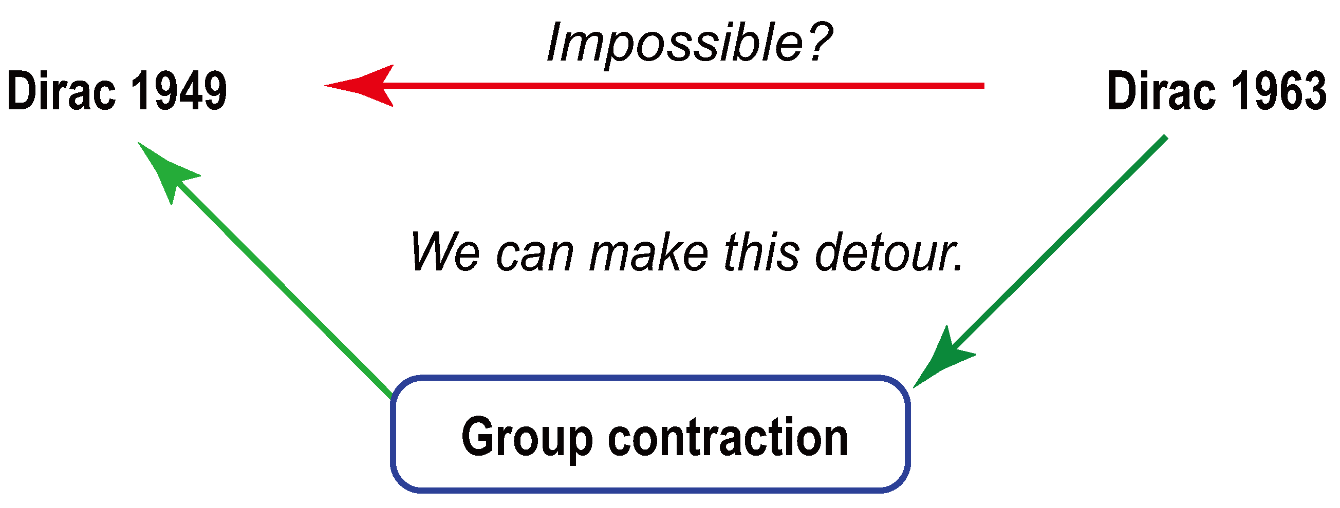
This paper is essentially based on Dirac’s paper published in 1949 and 1963 [1,2]. As is illustrated in Figure 2, we show here that the space-time symmetry of quantum mechanics mentioned in his 1949 paper is derivable from his two-oscillator system discussed in 1963. The route is the group contraction procedure of Inönü and Wigner [3].

Indeed, from 1927 Dirac made lifelong efforts to synthesize quantum mechanics and special relativity [4]. In 1949 and before, he treated quantum mechanics and special relativity as two separate scientific disciplines, and then in 1949 he attempted to synthesize them. Thus, it is of interest to see how Dirac’s ideas evolved during the period 1929–1949. We shall give a brief review of Dirac’s efforts during the period in Appendix A.

2. Symmetries of the Single-Mode States

Heisenberg’s uncertainty relation for a single Cartesian variable takes the form

$$[x,p]=i$$

(11)

with

$$p=-i\frac{\partial }{\partial x}.$$

Very often, it is more convenient to use the operators

$$a=\frac{1}{\sqrt{2}}(x+ip),a^{†}=\frac{1}{\sqrt{2}}(x-ip)$$

(12)

with

$$\left[a,a^{†}\right]=1.$$

(13)

This aspect is well known.

The representation based on a and $a^{†}$ is known as the harmonic oscillator representation of the uncertainty relation and is the basic language for the Fock space for particle numbers. This representation is therefore the basic language for quantum optics.

Let us next consider the quadratic forms: $aa,a^{†}{a}^{†},a{a}^{†}$, and $a^{†}a$. Then the linear combination

$$a{a}^{†}-a^{†}a=1,$$

(14)

according to the uncertainty relation. Thus, there are three independent quadratic forms, and we are led to the following two-by-two matrix:

$$\left(\begin{array}{cc}\left(a{a}^{†}+a^{†}a\right)/2& aa\\ a^{†}{a}^{†}& \left(a{a}^{†}+a^{†}a\right)/2\end{array}\right).$$

(15)

This matrix leads to the following three independent operators:

$$J_2=\frac{1}{2}\left(a{a}^{†}+a^{†}a\right),K_1=\frac{1}{2}\left(a^{†}{a}^{†}+aa\right),K_3=\frac{i}{2}\left(a^{†}{a}^{†}-aa\right).$$

(16)

They produce the following set of closed commutation relations:

$$\left[J_2,K_1\right]=-i{K}_3,\left[J_2,K_3\right]=i{K}_1,\left[K_1,K_3\right]=i{J}_2.$$

(17)

This set is commonly called the Lie algebra of the $Sp\left(2\right)$ group, locally isomorphic to the Lorentz group applicable to one time and two space coordinates.

The best way to study the symmetry property of these operators is to use the Wigner function for the ground-state oscillator which takes the form [5,6,7,8]

$$W(x,p)=\frac{1}{\pi }exp\left[-\left(x^2+p^2\right)\right].$$

(18)

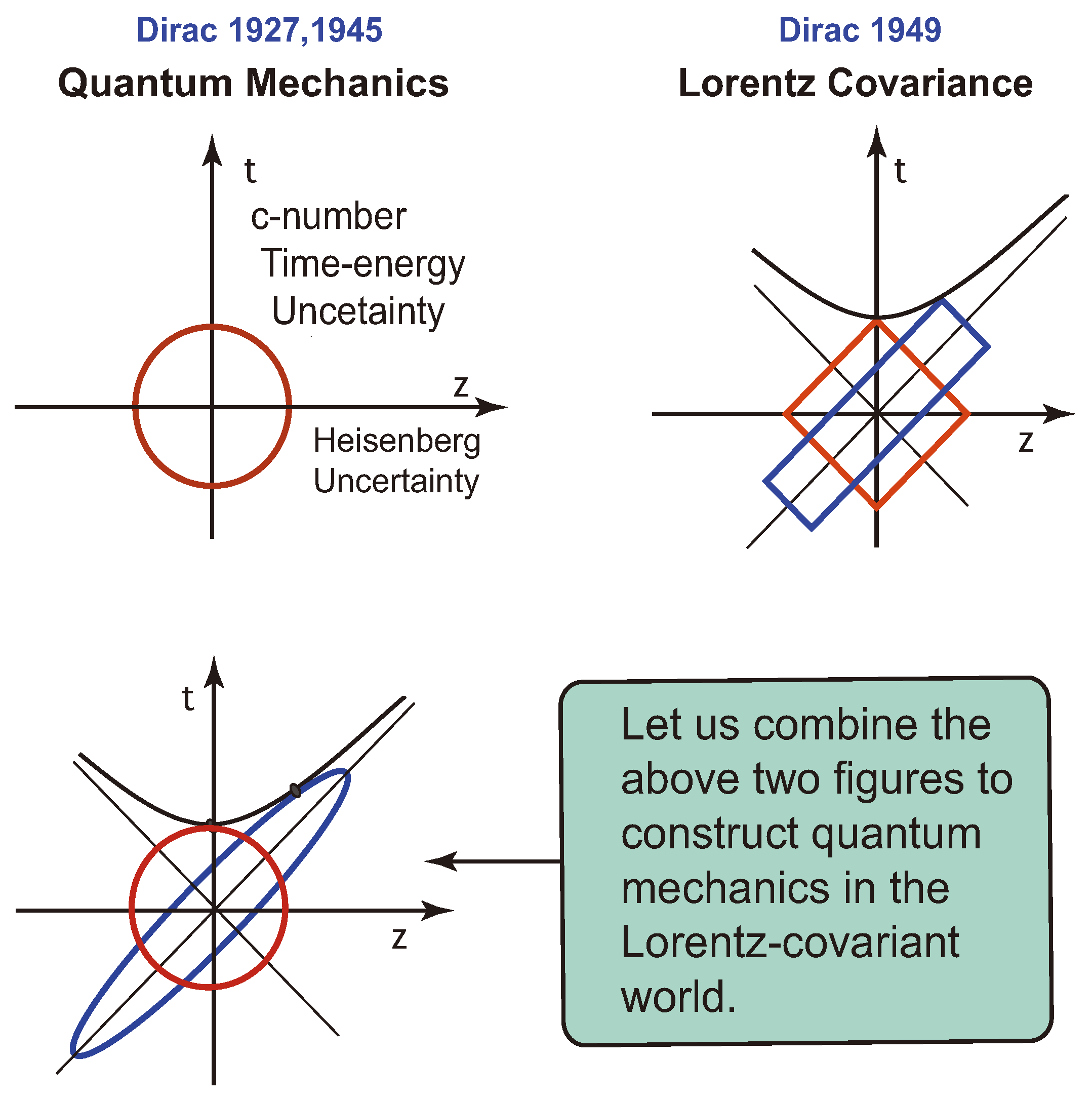
This distribution is concentrated in the circular region around the origin. Let us define the circle as

$$x^2+p^2=1.$$

(19)

We can use the area of this circle in the phase space of x and p as the minimum uncertainty. This uncertainty is preserved under rotations in the phase space and also under squeezing. These transformations can be written as

$$\left(\begin{array}{cc}cos\theta & -sin\theta \\ sin\theta & cos\theta \end{array}\right)\left(\begin{array}{c}x\\ p\end{array}\right),\left(\begin{array}{cc}{e}^{\eta }& 0\\ 0& e^{-\eta }\end{array}\right)\left(\begin{array}{c}x\\ p\end{array}\right),$$

(20)

respectively. The rotation and the squeeze are generated by

$$J_2=-i\left(x\frac{\partial }{\partial p}-p\frac{\partial }{\partial x}\right),K_1=-i\left(x\frac{\partial }{\partial x}-p\frac{\partial }{\partial p}\right).$$

(21)

If we take the commutation relation with these two operators, the result is

$$\left[J_2,K_1\right]=-i{K}_3,$$

(22)

with

$$K_3=-i\left(x\frac{\partial }{\partial p}+p\frac{\partial }{\partial x}\right).$$

(23)

Indeed, as before, these three generators form the closed set of commutation which form the Lie algebra of the $Sp\left(2\right)$ group, isomorphic to the Lorentz group applicable to two space and one time dimensions. This isomorphic correspondence is illustrated in Figure 3.

Let us consider the Minkowski space of $(x,y,z,t)$. It is possible to write three four-by-four matrices satisfying the Lie algebra of Equation (17). The three four-by-four matrices satisfying this set of commutation relations are:

$$J_2=\left(\begin{array}{cccc}0& 0& i& 0\\ 0& 0& 0& 0\\ i& 0& 0& 0\\ 0& 0& 0& 0\end{array}\right),K_1=\left(\begin{array}{cccc}0& 0& 0& i\\ 0& 0& 0& 0\\ 0& 0& 0& 0\\ i& 0& 0& 0\end{array}\right),K_3=\left(\begin{array}{cccc}0& 0& 0& 0\\ 0& 0& 0& 0\\ 0& 0& 0& i\\ 0& 0& i& 0\end{array}\right).$$

(24)

However, these matrices have null second rows and null second columns. Thus, they can generate Lorentz transformations applicable only to the three-dimensional space of $(x,z,t)$, while the y variable remains invariant. Thus, this single-oscillator system cannot describe what happens in the full four-dimensional Minkowski space.

Yet, it is interesting that the oscillator system can produce three different representations sharing the same Lie algebra with the (2 + 1)-dimensional Lorentz group, as shown in

Table 1. Transformation for the Gaussian function, in terms of harmonic oscillators, two-dimensional phase space, and the four-dimensional Minkowski space.

Generators	Oscillator	Phase Space	Lorentz
$J_2$	$\frac{1}{2}\left(a{a}^{†}+a^{†}a\right)$	$\frac{1}{2}{\sigma }_2$	$\left(\begin{array}{cccc}0& 0& i& 0\\ 0& 0& 0& 0\\ i& 0& 0& 0\\ 0& 0& 0& 0\end{array}\right)$
$K_1$	$\frac{1}{2i}\left(a^{†}{a}^{†}+aa\right)$	$\frac{i}{2}{\sigma }_1$	$\left(\begin{array}{cccc}0& 0& 0& i\\ 0& 0& 0& 0\\ 0& 0& 0& 0\\ i& 0& 0& 0\end{array}\right)$
$K_3$	$\frac{1}{2}\left(a^{†}{a}^{†}-aa\right),$	$\frac{i}{2}{\sigma }_3$	$\left(\begin{array}{cccc}0& 0& 0& 0\\ 0& 0& 0& 0\\ 0& 0& 0& i\\ 0& 0& i& 0\end{array}\right)$

.

3. Symmetries from Two Oscillators

In order to generate Lorentz transformations applicable to the full Minkowskian space, we may need two Heisenberg commutation relations. Indeed, Paul A. M. Dirac started this program in 1963 [2]. It is possible to write the two uncertainty relations using two harmonic oscillators as

$$\left[a_i,a_j^{†}\right]={\delta }_{ij},$$

(25)

with

$$a_i=\frac{1}{\sqrt{2}}\left(x_i+i{p}_i\right),a_i^{†}=\frac{1}{\sqrt{2}}\left(x_i-i{p}_i\right),$$

(26)

and

$$x_i=\frac{1}{\sqrt{2}}\left(a_i+a_i^{†}\right),p_i=\frac{i}{\sqrt{2}}\left(a_i^{†}-a_i\right),$$

(27)

where i and j could be 1 or 2.

As in the case of the two-by-two matrix given in Equation (15), we can consider the following four-by-four block-diagonal matrix if the oscillators are not coupled:

$$\left(\begin{array}{cccc}\left(a_1{a}_1^{†}+a_1^{†}{a}_1\right)/2& a_1{a}_1& 0& 0\\ a_1^{†}{a}_1^{†}& \left(a_1{a}_1^{†}+a_1^{†}{a}_1\right)/2& 0& 0\\ 0& 0& \left(a_2{a}_2^{†}+a_2^{†}{a}_2\right)/2& a_2{a}_2\\ 0& 0& a_2^{†}{a}_2^{†}& \left(a_2{a}_2^{†}+a_2^{†}{a}_2\right)/2\end{array}\right).$$

(28)

There are six generators in this matrix.

We are now interested in coupling them by filling in the off-diagonal blocks. The most general forms for this block are the following two-by-two matrix and its Hermitian conjugate:

$$\left(\begin{array}{cc}{a}_1^{†}{a}_2& a_1{a}_2\\ & \\ a_1^{†}{a}_2^{†}& a_1{a}_2^{†}\end{array}\right)$$

(29)

with four independent generators. This leads to the following four-by-four matrix with ten (6 + 4) generators:

$$\left(\begin{array}{cccc}\left(a_1{a}_1^{†}+a_1^{†}{a}_1\right)/2& a_1{a}_1& a_1^{†}{a}_2& a_1{a}_2\\ a_1^{†}{a}_1^{†}& \left(a_1{a}_1^{†}+a_1^{†}{a}_1\right)/2& a_1^{†}{a}_2^{†}& a_1{a}_2^{†}\\ a_1{a}_2^{†}& a_1{a}_2& \left(a_2{a}_2^{†}+a_2^{†}{a}_2\right)/2& a_2{a}_2\\ a_1^{†}{a}_2^{†}& a_1^{†}{a}_2& a_2^{†}{a}_2^{†}& \left(a_2{a}_2^{†}+a_2^{†}{a}_2\right)/2\end{array}\right).$$

(30)

With these ten elements, we can now construct the following four rotation-like generators:

$$\begin{array}{c}{J}_1=\frac{1}{2}\left(a_1^{†}{a}_2+a_2^{†}{a}_1\right),J_2=\frac{1}{2i}\left(a_1^{†}{a}_2-a_2^{†}{a}_1\right),\hfill \\ J_3=\frac{1}{2}\left(a_1^{†}{a}_1-a_2^{†}{a}_2\right),S_0=\frac{1}{2}\left(a_1^{†}{a}_1+a_2{a}_2^{†}\right),\hfill \end{array}$$

(31)

and six squeeze-like generators:

$$\begin{array}{c}{K}_1=-\frac{1}{4}\left(a_1^{†}{a}_1^{†}+a_1{a}_1-a_2^{†}{a}_2^{†}-a_2{a}_2\right),\hfill \\ K_2=+\frac{i}{4}\left(a_1^{†}{a}_1^{†}-a_1{a}_1+a_2^{†}{a}_2^{†}-a_2{a}_2\right),\hfill \\ K_3=+\frac{1}{2}\left(a_1^{†}{a}_2^{†}+a_1{a}_2\right),\hfill \end{array}$$

(32)

and

$$\begin{array}{c}{Q}_1=-\frac{i}{4}\left(a_1^{†}{a}_1^{†}-a_1{a}_1-a_2^{†}{a}_2^{†}+a_2{a}_2\right),\hfill \\ Q_2=-\frac{1}{4}\left(a_1^{†}{a}_1^{†}+a_1{a}_1+a_2^{†}{a}_2^{†}+a_2{a}_2\right),\hfill \\ Q_3=+\frac{i}{2}\left(a_1^{†}{a}_2^{†}-a_1{a}_2\right).\hfill \end{array}$$

(33)

There are now ten operators from Equations (31)–(33), and they satisfy the following Lie algebra as was noted by Dirac in 1963 [2]:

$$\begin{array}{c}[J_i,J_j]=i{ϵ}_{ijk}{J}_k,[J_i,K_j]=i{ϵ}_{ijk}{K}_k,\hfill \\ [J_i,Q_j]=i{ϵ}_{ijk}{Q}_k,[K_i,K_j]=[Q_i,Q_j]=-i{ϵ}_{ijk}{J}_k,\hfill \\ [K_i,Q_j]=-i{\delta }_{ij}{S}_0,[J_i,S_0]=0,[K_i,S_0]=-i{Q}_i,[Q_i,S_0]=i{K}_i.\hfill \end{array}$$

(34)

Dirac noted that this set is the same as the Lie algebra for the $O(3,2)$ de Sitter group, with ten generators. This is the Lorentz group applicable to the three-dimensional space with two time variables. This group plays a very important role in space-time symmetries.

In the same paper, Dirac pointed out that this set of commutation relations serves as the Lie algebra for the four-dimensional symplectic group commonly called $Sp\left(4\right)$. For a dynamical system consisting of two pairs of canonical variables $x_1,p_1$ and $x_2,p_2$, we can use the four-dimensional phase space with the coordinate variables defined as [9]

$$\left(x_1,p_1,x_2,p_2\right).$$

(35)

Then the four-by-four transformation matrix M applicable to this four-component vector is canonical if [10,11]

$$MJ\tilde{M}=J,$$

(36)

where $\tilde{M}$ is the transpose of the M matrix, with

$$J=\left(\begin{array}{cccc}0& 1& 0& 0\\ -1& 0& 0& 0\\ 0& 0& 0& 1\\ 0& 0& -1& 0\end{array}\right),$$

(37)

which we can write in the block-diagonal form as

$$J=i\left(\begin{array}{cc}I& 0\\ 0& I\end{array}\right){\sigma }_2,$$

(38)

where I is the unit two-by-two matrix.

According to this form of the J matrix, the area of the phase space for the $x_1$ and $p_1$ variables remains invariant, and the story is the same for the phase space of $x_2$ and $p_2.$

We can then write the generators of the $Sp\left(4\right)$ group as [12]

$$J_1=-\frac{1}{2}\left(\begin{array}{cc}0& I\\ I& 0\end{array}\right){\sigma }_2,J_2=\frac{i}{2}\left(\begin{array}{cc}0& -I\\ I& 0\end{array}\right)I,J_3=\frac{1}{2}\left(\begin{array}{cc}-I& 0\\ 0& I\end{array}\right){\sigma }_2,S_0=\frac{1}{2}\left(\begin{array}{cc}I& 0\\ 0& I\end{array}\right){\sigma }_2,$$

(39)

and

$$\begin{array}{c}{K}_1=\frac{i}{2}\left(\begin{array}{cc}I& 0\\ 0& -I\end{array}\right){\sigma }_1,K_2=\frac{i}{2}\left(\begin{array}{cc}I& 0\\ 0& I\end{array}\right){\sigma }_3,K_3=-\frac{i}{2}\left(\begin{array}{cc}0& I\\ I& 0\end{array}\right){\sigma }_1,\hfill \\ Q_1=-\frac{i}{2}\left(\begin{array}{cc}I& 0\\ 0& -I\end{array}\right){\sigma }_3,Q_2=\frac{i}{2}\left(\begin{array}{cc}I& 0\\ 0& I\end{array}\right){\sigma }_1,Q_3=\frac{i}{2}\left(\begin{array}{cc}0& I\\ I& 0\end{array}\right){\sigma }_3.\hfill \end{array}$$

(40)

Among these ten matrices, six of them are in block-diagonal form. They are $S_0,J_3,K_1,K_2,Q_1,$ and $Q_2.$ In the language of two harmonic oscillators, these generators do not mix up the first and second oscillators. There are six of them because each operator has three generators for its own $Sp\left(2\right)$ symmetry. These generators, together with those in the oscillator representation, are tabulated in

Table 2. Transformation generators for the two-oscillator system.

Generators	Two Oscillators	Phase Space
$J_1$	$\frac{1}{2}\left(a_1^{†}{a}_2+a_2^{†}{a}_1\right)$	$-\frac{1}{2}\left(\begin{array}{cc}0& I\\ I& 0\end{array}\right){\sigma }_2$
$J_2$	$\frac{1}{2i}\left(a_1^{†}{a}_2-a_2^{†}{a}_1\right)$	$\frac{i}{2}\left(\begin{array}{cc}0& -I\\ I& 0\end{array}\right)I$
$J_3$	$\frac{1}{2}\left(a_1^{†}{a}_1-a_2^{†}{a}_2\right),$	$\frac{1}{2}\left(\begin{array}{cc}-I& 0\\ 0& I\end{array}\right){\sigma }_2$
$S_0$	$\frac{1}{2}\left(a_1^{†}{a}_1+a_2{a}_2^{†}\right),$	$\frac{1}{2}\left(\begin{array}{cc}I& 0\\ 0& I\end{array}\right){\sigma }_2$
$K_1$	$-\frac{1}{4}\left(a_1^{†}{a}_1^{†}+a_1{a}_1-a_2^{†}{a}_2^{†}-a_2{a}_2\right)$	$\frac{i}{2}\left(\begin{array}{cc}I& 0\\ 0& -I\end{array}\right){\sigma }_1$
$K_2$	$+\frac{i}{4}\left(a_1^{†}{a}_1^{†}-a_1{a}_1+a_2^{†}{a}_2^{†}-a_2{a}_2\right)$	$\frac{i}{2}\left(\begin{array}{cc}I& 0\\ 0& I\end{array}\right){\sigma }_3$
$K_3$	$\frac{1}{2}\left(a_1^{†}{a}_2^{†}+a_1{a}_2\right)$	$-\frac{i}{2}\left(\begin{array}{cc}0& I\\ I& 0\end{array}\right){\sigma }_1$
$Q_1$	$-\frac{i}{4}\left(a_1^{†}{a}_1^{†}-a_1{a}_1-a_2^{†}{a}_2^{†}+a_2{a}_2\right)$	$-\frac{i}{2}\left(\begin{array}{cc}I& 0\\ 0& -I\end{array}\right){\sigma }_3$
$Q_2$	$-\frac{1}{4}\left(a_1^{†}{a}_1^{†}+a_1{a}_1+a_2^{†}{a}_2^{†}+a_2{a}_2\right)$	$\frac{i}{2}\left(\begin{array}{cc}I& 0\\ 0& I\end{array}\right){\sigma }_1$
$Q_3$	$\frac{i}{2}\left(a_1^{†}{a}_2^{†}-a_1{a}_2\right)$	$\frac{1}{2}\left(\begin{array}{cc}I& 0\\ 0& I\end{array}\right){\sigma }_2$

.

The off-diagonal matrix $J_2$ couples the first and second oscillators without changing the overall volume of the four-dimensional phase space. However, in order to construct the closed set of commutation relations, we need the three additional generators: $J_1,K_3,$ and $Q_3.$ The commutation relations given in Equations (34) are clearly consequences of Heisenberg’s uncertainty relations.

As for the $O(3,2)$ group, the generators are five-by-five matrices, applicable to $(x,y,z,t,s)$, where t and s are time-like variables. These matrices can be written as

$$\begin{array}{c}{J}_1=\left(\begin{array}{ccccc}0& 0& 0& 0& 0\\ 0& 0& -i& 0& 0\\ 0& i& 0& 0& 0\\ 0& 0& 0& 0& 0\\ 0& 0& 0& 0& 0\end{array}\right),J_2=\left(\begin{array}{ccccc}0& 0& i& 0& 0\\ 0& 0& 0& 0& 0\\ -i& 0& 0& 0& 0\\ 0& 0& 0& 0& 0\\ 0& 0& 0& 0& 0\end{array}\right),J_3=\left(\begin{array}{ccccc}0& -i& 0& 0& 0\\ i& 0& 0& 0& 0\\ 0& 0& 0& 0& 0\\ 0& 0& 0& 0& 0\\ 0& 0& 0& 0& 0\end{array}\right),\hfill \\ K_1=\left(\begin{array}{ccccc}0& 0& 0& i& 0\\ 0& 0& 0& 0& 0\\ 0& 0& 0& 0& 0\\ i& 0& 0& 0& 0\\ 0& 0& 0& 0& 0\end{array}\right),K_2=\left(\begin{array}{ccccc}0& 0& 0& 0& 0\\ 0& 0& 0& i& 0\\ 0& 0& 0& 0& 0\\ 0& i& 0& 0& 0\\ 0& 0& 0& 0& 0\end{array}\right),K_3=\left(\begin{array}{ccccc}0& 0& 0& 0& 0\\ 0& 0& 0& 0& 0\\ 0& 0& 0& i& 0\\ 0& 0& i& 0& 0\\ 0& 0& 0& 0& 0\end{array}\right),\hfill \\ Q_1=\left(\begin{array}{ccccc}0& 0& 0& 0& i\\ 0& 0& 0& 0& 0\\ 0& 0& 0& 0& 0\\ 0& 0& 0& 0& 0\\ i& 0& 0& 0& 0\end{array}\right),Q_2=\left(\begin{array}{ccccc}0& 0& 0& 0& 0\\ 0& 0& 0& 0& i\\ 0& 0& 0& 0& 0\\ 0& 0& 0& 0& 0\\ 0& i& 0& 0& 0\end{array}\right),Q_3=\left(\begin{array}{ccccc}0& 0& 0& 0& 0\\ 0& 0& 0& 0& 0\\ 0& 0& 0& 0& i\\ 0& 0& 0& 0& 0\\ 0& 0& i& 0& 0\end{array}\right),\hfill \\ S_0=\left(\begin{array}{ccccc}0& 0& 0& 0& 0\\ 0& 0& 0& 0& 0\\ 0& 0& 0& 0& 0\\ 0& 0& 0& 0& -i\\ 0& 0& 0& i& 0\end{array}\right).\hfill \end{array}$$

(41)

Next, we are interested in eliminating all the elements in the fifth row. The six generators $J_i$ and $K_i$ are not affected by this operation, but $Q_1,Q_2,Q_3,$ and $S_0$ become

$$\begin{array}{c}{P}_1=\left(\begin{array}{ccccc}0& 0& 0& 0& i\\ 0& 0& 0& 0& 0\\ 0& 0& 0& 0& 0\\ 0& 0& 0& 0& 0\\ 0& 0& 0& 0& 0\end{array}\right),P_2=\left(\begin{array}{ccccc}0& 0& 0& 0& 0\\ 0& 0& 0& 0& i\\ 0& 0& 0& 0& 0\\ 0& 0& 0& 0& 0\\ 0& 0& 0& 0& 0\end{array}\right),P_3=\left(\begin{array}{ccccc}0& 0& 0& 0& 0\\ 0& 0& 0& 0& 0\\ 0& 0& 0& 0& i\\ 0& 0& 0& 0& 0\\ 0& 0& 0& 0& 0\end{array}\right),\hfill \\ P_0=\left(\begin{array}{ccccc}0& 0& 0& 0& 0\\ 0& 0& 0& 0& 0\\ 0& 0& 0& 0& 0\\ 0& 0& 0& 0& -i\\ 0& 0& 0& 0& 0\end{array}\right),\hfill \end{array}$$

(42)

respectively. While $J_i$ and $K_i$ generate Lorentz transformations on the four dimensional Minkowski space, these $Q_i$ and $S_0$ in the form of the $P_i,P_0$ matrices generate translations along the $x,y,z,$ and t directions respectively. We shall study this aspect in detail in Section 4.

4. Contraction of $\mathit{O}\mathbf{(}\mathbf{3}\mathbf{,}\mathbf{2}\mathbf{)}$ to the Inhomogeneous Lorentz Group

We can contract $O(3,2)$ according to the procedure introduced by Inönü and Wigner [3]. They introduced the procedure for transforming the four-dimensional Lorentz group into the three-dimensional Galilei group. Here, we shall contract the boost generators belonging to the time-like s variable, $Q_i$, along with the rotation generator between the two time-like variables, $S_0$.

Here, we illustrate the Inönü-Wigner procedure using the concept of squeeze transformations. For this purpose, let us introduce the squeeze matrix

$$C\left(ϵ\right)=\left(\begin{array}{ccccc}1/ϵ& 0& 0& 0& 0\\ 0& 1/ϵ& 0& 0& 0\\ 0& 0& 1/ϵ& 0& 0\\ 0& 0& 0& 1/ϵ& 0\\ 0& 0& 0& 0& ϵ\end{array}\right).$$

(43)

This matrix commutes with $J_i$ and $K_i$. The story is different for $Q_i$ and $S_0$.

For $Q_1$,

$$C{Q}_1{C}^{-1}=\left(\begin{array}{ccccc}0& 0& 0& 0& i/{ϵ}^2\\ 0& 0& 0& 0& 0\\ 0& 0& 0& 0& 0\\ 0& 0& 0& 0& 0\\ i{ϵ}^2& 0& 0& 0& 0\end{array}\right),$$

(44)

which, in the limit of small $ϵ$, becomes

$$Q_1^{\prime }=\left(\begin{array}{ccccc}0& 0& 0& 0& i/{ϵ}^2\\ 0& 0& 0& 0& 0\\ 0& 0& 0& 0& 0\\ 0& 0& 0& 0& 0\\ 0& 0& 0& 0& 0\end{array}\right).$$

(45)

We then make the inverse squeeze transformation:

$$C^{-1}{Q}_1^{\prime }C=\left(\begin{array}{ccccc}0& 0& 0& 0& i\\ 0& 0& 0& 0& 0\\ 0& 0& 0& 0& 0\\ 0& 0& 0& 0& 0\\ 0& 0& 0& 0& 0\end{array}\right).$$

(46)

Thus, we can write this contraction procedure as

$$P_1=\underset{ϵ\to 0}{lim}\left({ϵ}^{2}C{Q}_1{C}^{-1}\right),$$

(47)

where the explicit five-by-five matrix is given in Equation (42). Likewise

$$P_2=\underset{ϵ\to 0}{lim}\left({ϵ}^{2}C{Q}_2{C}^{-1}\right),P_3=\underset{ϵ\to 0}{lim}\left({ϵ}^{2}C{Q}_3{C}^{-1}\right),P_0=\underset{ϵ\to 0}{lim}\left({ϵ}^{2}C{S}_0{C}^{-1}\right).$$

(48)

These four contracted generators lead to the five-by-five transformation matrix, as can be seen from

$$exp\left\{-i\left(a{P}_1+b{P}_2+c{P}_3+d{P}_0\right)\right\}$$

(49)

performing translations in the four-dimensional Minkowski space:

$$\left(\begin{array}{ccccc}1& 0& 0& 0& a\\ 0& 1& 0& 0& b\\ 0& 0& 1& 0& c\\ 0& 0& 0& 1& -d\\ 0& 0& 0& 0& 1\end{array}\right)\left(\begin{array}{c}x\\ y\\ z\\ t\\ 1\end{array}\right)=\left(\begin{array}{c}x+a\\ y+b\\ z+c\\ t-d\\ 1\end{array}\right).$$

(50)

In this way, the space-like directions are translated and the time-like t component is shortened by an amount d. This means the group $O(3,2)$ derivable from the Heisenberg’s uncertainty relations becomes the inhomogeneous Lorentz group governing the Poincaré symmetry for quantum mechanics and quantum field theory. These matrices correspond to the differential operators

$$P_x=-i\frac{\partial }{\partial x},P_y=-i\frac{\partial }{\partial y},P_z=-i\frac{\partial }{\partial z},P_0=i\frac{\partial }{\partial t},$$

(51)

respectively. These translation generators correspond to the Lorentz-covariant four-momentum variable with

$$p_1^2+p_2^2+p_3^2-p_0^2=\mathrm{constant}.$$

(52)

This energy-momentum relation is widely known as Einstein’s $E=m{c}^2$.

5. Concluding Remarks

According to Dirac [1], the problem of finding a Lorentz-covariant quantum mechanics reduces to the problem of finding a representation of the inhomogeneous Lorentz group. Again, according to Dirac [2], it is possible to construct the Lie algebra of the group $O(3,2)$ starting from two oscillators. We have shown in our earlier paper [12] that this $O(3,2)$ group can be contracted to the inhomogeneous Lorentz group according to the group contraction procedure introduced by Inönü and Wigner [3].

In this paper, we noted first that the symmetry of a single oscillator is generated by three generators. Two independent oscillators thus have six generators. We have shown that there are four additional generators needed for the coupling of the two oscillators. Thus there are ten generators. These ten generators can then be linearly combined to produce ten generators which were spelled out in Dirac’s 1963 paper.

For the two-oscillator system, there are four step-up and step-down operators. There are therefore sixteen quadratic forms [9]. Among those, only ten of them are in Dirac’s 1963 paper [2]. Why ten? Dirac needed those ten to construct the Lie algebra for the $O(3,2)$ group. At the end of the same paper, he stated that this Lie algebra is the same as that for the $Sp\left(4\right)$ group, which preserves the minimum uncertainty for each oscillator.

In this paper, we started with the block-diagonal matrix given in Equation (28) for two totally independent oscillators with six independent generators. We then added one two-by-two Hermitian matrix of Equation (29) with four generators for the off-diagonal blocks. The result is the four-by-four Hermitian matrix given in Equation (30). This four-by-four Hermitian matrix has ten independent operators which can be linearly combined to the ten operators chosen by Dirac. Thus, in this paper, we have shown how the two-oscillators are coupled, and how this coupling introduces additional symmetries.

Paul A. M. Dirac made life-long efforts to make quantum mechanics consistent with special relativity, starting from 1927 [4]. While we exploited the contents of his paper published in 1963 [2], it is of interest to review his earlier efforts. In his earlier papers, Dirac started with quantum mechanics and special relativity as two different branches of science based on two different mathematical bases.

In this paper, based on Dirac’s two papers [1,2], we concluded that both quantum mechanics and special relativity can be derived from the same mathematical base. A brief review of Dirac’s earlier efforts is given in Appendix A.

References

1. Dirac, P.A.M. Forms of Relativistic Dynamics. Rev. Mod. Phys. 1949, 21, 392–399. [Google Scholar] [CrossRef] [Green Version]
2. Dirac, P.A.M. A Remarkable Representation of the 3 + 2 de Sitter Group. J. Math. Phys. 1963, 4, 901–909. [Google Scholar] [CrossRef]
3. Inönü, E.; Wigner, E.P. On the Contraction of Groups and their Representations. Proc. Natl. Acad. Sci. USA 1953, 39, 510–524. [Google Scholar] [CrossRef] [PubMed]
4. Dirac, P.A.M. The Quantum Theory of the Emission and Absorption of Radiation. Proc. R. Soc. (London) 1927, A114, 243–265. [Google Scholar] [CrossRef]
5. Han, D.; Kim, Y.S.; Noz, M.E. Linear canonical transformations of coherent and squeezed states in the Wigner phase space. Phys. Rev. A 1988, 37, 807–814. [Google Scholar] [CrossRef] [PubMed]
6. Kim, Y.S.; Wigner, E.P. Canonical transformation in quantum mechanics. Am. J. Phys. 1990, 58, 439–447. [Google Scholar] [CrossRef]
7. Kim, Y.S.; Noz, M.E. Phase Space Picture of Quantum Mechanics; World Scientific Publishing Company: Singapore, 1991. [Google Scholar]
8. Dodonov, V.V.; Man’ko, V.I. Theory of Nonclassical States of Light; Taylor & Francis: London, UK; New York, NY, USA, 2003. [Google Scholar]
9. Han, D.; Kim, Y.S.; Noz, M.E. O(3, 3)-like Symmetries of Coupled Harmonic Oscillators. J. Math. Phys. 1995, 36, 3940–3954. [Google Scholar] [CrossRef]
10. Abraham, R.; Marsden, J.E. Foundations of Mechanics, 2nd ed.; Benjamin Cummings: Reading, MA, USA, 1978. [Google Scholar]
11. Goldstein, H. Classical Mechanics, 2nd ed.; Addison-Wesley: Reading, MA, USA, 1980. [Google Scholar]
12. Başkal, S.; Kim, Y.S.; Noz, M.E. Poincaré Symmetry from Heisenberg’s Uncertainty Relations. Symmetry 2019, 11, 409. [Google Scholar] [CrossRef]
13. Kim, Y.S.; Noz, M.E.; Oh, S.H. Representations of the Poincaré group for relativistic extended hadrons. J. Math. Phys. 1979, 20, 1341–1344. [Google Scholar] [CrossRef]
14. Wigner, E. On unitary representations of the inhomogeneous Lorentz group. Ann. Math. 1939, 40, 149–204. [Google Scholar] [CrossRef]
15. Dirac, P.A.M. Unitary Representations of the Lorentz Group. Proc. R Soc. (London) 1945, A183, 284–295. [Google Scholar]
16. Gell-Mann, M. A Schematic Model of Baryons and Mesons. Phys. Lett. 1964, 8, 214–215. [Google Scholar] [CrossRef]
17. Feynman, R.P. Very High-Energy Collisions of Hadrons. Phys. Rev. Lett. 1969, 23, 1415–1417. [Google Scholar] [CrossRef] [Green Version]
18. Bjorken, J.D.; Paschos, E.A. Electron-Proton and γ-Proton Scattering and the Structure of the Nucleon. Phys. Rev. 1969, 185, 1975–1982. [Google Scholar] [CrossRef]
19. Kim, Y.S.; Noz, M.E. Covariant harmonic oscillators and the parton picture. Phys. Rev. D 1977, 15, 335–338. [Google Scholar] [CrossRef]
20. Başkal, S.; Kim., Y.S.; Noz, M.E. Physics of the Lorentz Group, IOP Concise Physics; Morgan & Claypool Publisher: San Rafael, CA, USA; IOP Publishing: Bristol, UK, 2015. [Google Scholar]
Figure 1. The Inönü–Wigner contraction procedure interpreted as squeeze transformations. In (a), the square becomes a narrow rectangle during the squeeze process. When the rectangle becomes narrow enough, the point A can be moved to the horizontal axis. Then, the inverse squeeze brings back the rectangle to the original shape. The point A remains on the horizontal axis. In (b), both the hyperbola and the circle become flattened to the horizontal axis, during the initial squeeze. The point on the curve moves to the horizontal axis. This point moves back to its finite position during the inverse squeeze.
Quantumrep 01 00021 g001
Figure 2. According to Dirac’s 1949 paper, the task of constructing quantum mechanics is essentially constructing a representation of the inhomogeneous Lorentz group. In his 1963 paper, Dirac constructed the Lie algebra of the O ( 3 , 2 ) de Sitter group from the algebra of two harmonic oscillators, which is a direct consequence of Heisenberg’s uncertainty commutation relations. It is possible to derive the Lie algebra of the inhomogeneous Lorentz group from that of O ( 3 , 2 ) using the group-contraction procedure of Inönü and Wigner [3].
Quantumrep 01 00021 g002
Figure 3. Rotations and squeezes in the phase space produced by the S p ( 2 ) transformations. The squeeze along the x direction corresponds to the Lorentz boost along the z direction, while the squeeze along the 45 angle corresponds to the boost along the x direction. The rotation by 45 corresponds to the rotation by 90 around the y axis.
Quantumrep 01 00021 g003