A Full-Parameter Calibration Method for an RINS/CNS Integrated Navigation System in High-Altitude Drones

Abstract

High-altitude long-endurance (HALE) UAVs require navigation payloads that are both fully autonomous and lightweight. This paper presents a full-parameter calibration method for a dual-axis rotational-modulation RINS/CNS integrated system in which the IMU is mounted on a two-axis indexing mechanism and the reconnaissance camera is reused as the star sensor. We establish a unified error propagation model that simultaneously covers IMU device errors (bias, scale, cross-axis/installation), gimbal non-orthogonality and encoder angle errors, and camera exterior/interior parameters (EOPs/IOPs), including Brown–Conrady distortion. Building on this model, we design an error-decoupled calibration path that exploits (i) odd/even symmetry under inner-axis scans, (ii) basis switching via outer-axis waypoints, and (iii) frequency tagging through rate-limited triangular motions. A piecewise-constant system (PWCS)/SVD analysis quantifies segment-wise observability and guides trajectory tuning. Simulation and hardware-in-the-loop results show that all parameter groups converge primarily within the segments that excite them; the final relative errors are typically ≤5% in simulation and 6–$16\%$ with real IMU/gimbal data and catalog-based star pixels.

1. Introduction

High-altitude long-endurance (HALE) UAVs are increasingly deployed for persistent ISR, disaster response, and scientific sensing where GNSS may be denied or intermittently available [1,2]. In these scenarios, fully autonomous navigation with bounded drift is critical. Strapdown inertial navigation systems (SINS) provide autonomy but suffer from error growth; celestial navigation systems (CNS) offer drift-free attitude (and, in some architectures, position) [3,4] updates with low duty-cycle sensing. Rotational-modulation inertial systems (RINS) further suppress inertial device errors by periodically reorienting the IMU so that bias- and misalignment-induced terms average out over a cycle [5,6]. Combining these ideas, a dual-axis rotational INS/CNS (RINS/CNS) mounted on the reconnaissance gimbal can, in principle, deliver high-accuracy, reference-free navigation with limited mass overhead.

Recent work in the literature has advanced both the SINS/CNS fusion algorithms and the system-level self-calibration of dual-axis RINS. On the CNS side, improved mathematical-horizon-based attitude/position references and robust filtering have been reported for aerospace and planetary applications [7,8]. On the RINS side, system-level self-calibration methods that exploit deliberate rotation sequences to render inertial and installation parameters observable have significantly shortened calibration time and improved repeatability [9,10]. For star sensors (the “camera” in the INS/CNS context), the on-orbit calibration and self-calibration of intrinsics/extrinsics are being revisited with modern optimization and observability tools to mitigate performance degradation after deployment [11]. These developments make a unified, flight-realistic, full-parameter calibration of a gimbaled RINS/CNS both timely and practically relevant.

Recent work has accelerated system-level calibration by leveraging rotation-induced invariants and well-conditioned motion schemes. Sun formulate navigation errors as invariant elements and use backtracking navigation to realize a fast, equipment-free self-calibration for dual-axis RINS; their analysis clarifies how the invariant form improves numerical conditioning and convergence under large misalignment [9]. Wei et al. report an improved system-level scheme that jointly estimates IMU device errors and gimbal geometric errors, with a motion plan that mitigates parameter collinearity in the normal equations [10]. Temperature-sensitive non-orthogonality is explicitly modeled and compensated in [12], showing that coupling terms can be rendered observable without environmental chambers by designing temperature-varying excitation segments. Earlier but still influential works explored asynchronous-axis rotation and multi-position strategies for separating inner/outer-axis installation errors and scale/cross terms, laying the foundation for today’s observability-guided paths [13,14]. Together, these studies converge on two themes: (a) system-level estimation is preferable to piecemeal device-only calibration; and (b) designed excitation (multi-axis, multi-basis) is crucial for well-conditioned identification.

One line of research examines how rotational modulation moves IMU biases and misalignments into trigonometric forms so that they can be averaged or demodulated. Comparative studies confirm that encoder angle errors and gimbal non-orthogonality enter the same attitude pathway as IMU installation errors, and hence must be treated jointly [9,10]. Moving-base and lever-arm effects have also been analyzed: when rotation centers are offset from the sensor triad, additional coupling appears in the velocity/attitude residuals and must be included in the state vector for unbiased estimation [13]. Recent practical reports emphasize rate-limited triangular waves and basis switching to balance the star visibility, rate limits, and observability of axis-specific terms (e.g., inner encoder vs. outer encoder) [9].

On the CNS side, mathematical-horizon-based references and adaptive fusion have improved robustness under partial sky coverage or sky/background interference. Yang et al. developed an improved mathematical horizon reference that stabilizes attitude and heading updates within an integrated SINS/CNS filter [7]. Li et al. designed a robust adaptive scheme (validated on Mars-rover-like scenarios) that demonstrated resilience against uncertain CNS noise and modeling errors [8]. Complementary approaches introduce prediction/detection modules (e.g., LSTM) to screen degraded CNS attitudes, acting as backup when stars are intermittently lost [15]. Adaptive variants of the Sage–Husa filter have also been shown to improve fusion stability when CNS update statistics vary [16]. Collectively, these works show that CNS can be made sufficiently reliable (even at low duty cycles) to serve as the primary attitude aid for RINS self-calibration in flight-realistic conditions.

For the imaging unit, the pinhole model with Brown–Conrady distortion remains standard; what has evolved is the on-orbit calibration/self-calibration pipeline and the treatment of couplings between intrinsics (IOPs) and boresight/extrinsics (EOPs). Fu et al. review attitude-dependent vs. attitude-independent on-orbit calibration and show how coupling between IOPs and EOPs can be reduced by design, with convergence under realistic centroid noise and FOV constraints [11]. Laboratory and on-orbit methods based on dual vector/attitude constraints and global optimization continue to improve geometric accuracy when star fields are sparse or the FOV is narrow [17,18]. In tightly coupled stellar–inertial integration, prediction-residual constructs such as star centroid prediction error (SCPE) offer additional observables and can stabilize camera parameters during maneuvers [19]. These results indicate that full camera calibration (IOP/EOP/distortion) is feasible without metrology-grade fixtures, provided that the image coverage has a center-to-edge span and that boresight is co-estimated with gimbal parameters.

Bringing the threads together, recent SINS/CNS/RINS reports advocate for the joint estimation of (i) IMU bias/scale/cross and installation, (ii) gimbal non-orthogonality and encoder angle errors, and (iii) camera IOPs/EOPs with lens distortion—using a single, carefully designed dual-axis path respecting rate limits and star visibility. The remaining challenges are path-dependent observability (e.g., outer-encoder parameters remain unobservable without dedicated outer-axis motion) and avoiding over-parameterization, which harms conditioning. The consensus is that multi-basis excitation, odd/even symmetry under inner scans, and frequency tagging for outer-axis motion offer practical decoupling tools that make a full-parameter solution attainable within short calibration windows in the field. Beyond HALE applications, there is rapidly growing interest in space–air–ground collaborative positioning, navigation, and timing architectures for the low-altitude economy [20]. Large AI models are also being explored to support intelligent low-altitude platforms and services [21]. In such scenarios, UAVs often carry multi-sensor navigation payloads (inertial, vision, GNSS, etc.) whose performance also depends critically on system-level calibration. Although our present focus is on a HALE-oriented RINS/CNS payload, the decoupling principles and path-design ideas in this paper are applicable to low-altitude systems with appropriate adaptation of the measurement model and excitation constraints.

Despite the above progress, two gaps remain for dual-axis RINS/CNS used on HALE UAVs:

G1—Error coupling across subsystems. Gimbal non-orthogonality and encoder angle errors enter the same attitude pathway as camera EOPs and, through projection, mix with IMU installation and cross-axis terms. Without careful design, these parameters are only weakly separable in batch or sequential estimators. G2—Path-dependent observability. The identifiability of many parameters is highly segment-dependent: inner-axis parameters require inner-axis excitation; outer-axis encoder errors require outer-axis motion; camera intrinsics/distortion require center-to-edge FOV coverage. Yet, many reported paths are designed for one subsystem rather than the full stack.

This paper presents a full-parameter calibration method and a decoupled excitation path for a dual-axis RINS/CNS integrated navigation system. The main contributions of this study are as follows:

• Unification of the propagation of gimbal non-orthogonality/encoder errors, IMU device errors, and camera IOPs/EOPs (with Brown–Conrady distortion) in one linearized measurement model tied to star-pixel residuals, enabling consistent EKF-based estimation.
• Decoupling of error sources at the measurement level using three complementary mechanisms: (i) odd/even symmetry under inner-axis scans to isolate inner encoder error from quasi-DC terms (EOPs, outer encoder, non-orthogonality); (ii) basis switching via outer-axis waypoints to rotate the Jacobian subspaces and reduce parameter collinearity; and (iii) frequency tagging through rate-limited triangular motions to isolate outer-axis encoder errors. This yields block-diagonal normal equations to the first order and improves conditioning relative to single-purpose paths.
• Quantification of segment-wise observability via a PWCS/SVD framework and Fisher Information Matrices, allowing each segment to be justified according to its contribution to the parameter block of interest.

Compared with existing dual-axis RINS self-calibration schemes, which jointly estimate IMU device and gimbal geometric errors but assume a separately calibrated star sensor, the present work explicitly incorporates camera IOPs/EOPs and distortion into the same state vector and pixel measurement model. Relative to star-sensor self-/on-orbit calibration methods, which focus on imaging geometry alone, our method co-estimates IMU, gimbal, and camera parameters using a single dual-axis trajectory that respects the mechanical and visibility constraints of HALE UAVs. The rest of this paper is organized as follows: Section 2 formulates coordinate frames and error models for the gimbal/IMU/camera cascade. Section 3 builds the star-pixel-based measurement model and filter structure. Section 4 designs the error-decoupled calibration path under mechanical/visibility constraints. Section 5 and Section 6 present simulation and semi-physical simulation results, respectively. Section 7 concludes by discussing limitations and future work.

2. System Error and Propagation

2.1. Notation and Nomenclature

Frames: n (navigation, ENU), b (body), s (IMU triad), $h1/h2$ (inner/outer gimbal), and c (camera). A DCM ${\mathbf{C}}_b^a$ maps a vector from frame b to frame a, with

$${\mathbf{C}}_c^a={\mathbf{C}}_b^a{\mathbf{C}}_c^b,{\left({\mathbf{C}}_b^a\right)}^{-1}={\left({\mathbf{C}}_a^b\right)}^{\top }$$

for a small rotation $\delta \mathit{\theta }$, $\delta \mathbf{C}\approx \mathbf{I}-[\delta \mathit{\theta }\times ]$, where $[·\times ]$ denotes the skew-symmetric cross-product matrix. Commanded gimbal angles: $\alpha$ (inner, about $+X_b$) and $\beta$ (outer, about $+Z_b$). The main frames and symbols used in this paper are summarized in Table 1.

Table 1. Notation and frame-related variables.

Symbol	Meaning
$b,n,s,h1$	Body, navigation (ENU), sensor, inner gimbal frame
$h2,c$	Outer gimbal, camera frame
${\mathbf{C}}_b^a$	DCM: maps vectors from b to a
$\alpha ,\beta$	Inner/outer commanded angles
$\delta \alpha ,\delta \beta$	Inner/outer encoder angle errors
${\theta }_x,{\theta }_y,{\theta }_z,\phi$	Gimbal non-orthogonality (four-parameter model)
${\epsilon }^s,{𝛁}^s$	Gyro/accelerometer constant biases (sensor frame)
$\Delta {\mathbf{K}}_{g/a}$	Gyro/accelerometer scale factors (diagonal)
$\Delta {\mathbf{A}}_{g/a}$	Gyro/accelerometer cross-axis/installation (first-order)
$(f_x,f_y,c_x,c_y,s)$	Camera intrinsics (with optional pixel skew s)
$(k_1,k_2,p_1,p_2)$	Brown–Conrady radial/tangential distortion
${\mathbf{R}}_{BC}$	Camera-to-body boresight DCM (EOP)

2.2. System and Reference Frames

The payload consists of a dual-axis indexing mechanism, an IMU (three gyros, three accelerometers), and a camera reused as a star sensor (Figure 1 and Figure 2). The nominal sensor-to-body cascade is

$${\mathbf{C}}_s^b(\alpha ,\beta )={\mathbf{C}}_{h1}^b\left(\alpha \right){\mathbf{C}}_{h2}^{h1}{\mathbf{C}}_s^{h2}\left(\beta \right).$$

(1)

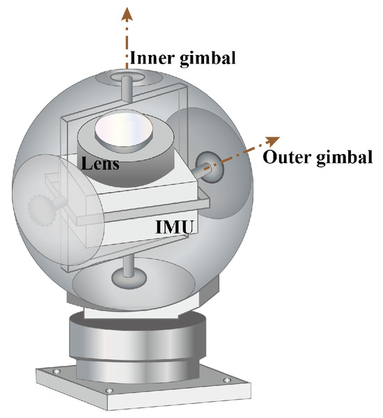
Figure 1. System structure of the dual-axis RINS/CNS payload.

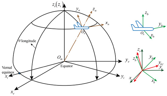
Figure 2. Coordinate frames and transformations.

2.3. Gimbal Errors

Under ideal conditions, the h1 system coincides with the h2 system, and the rotational-axis system coincides with the s system. However, in practical systems, factors such as environmental variations, assembly tolerances, and component ageing lead to a deterioration in the orthogonality between axis systems, thereby affecting navigation accuracy and rotational modulation performance. In Reference [22], the non-orthogonality of the coordinate systems is modeled in two parts: the first describes the non-orthogonal angles ${\theta }_x$, ${\theta }_y$, ${\theta }_z$ between the s system and the initial inner-axis coordinate system; the second describes the non-orthogonality between the inner and outer axes along the z-direction, characterised by the angle $\varphi$. The relationship between each non-orthogonal angle and the axis system is shown in Figure 3. Introducing the initial internal axis coordinate system $h_1^0$ facilitates description; thus, the error matrix caused by non-orthogonal angle could be written as follows:

$${\mathbf{C}}_s^{h{1}^0}=\left[\begin{array}{ccc}1& {\theta }_z& -{\theta }_y\\ -{\theta }_z& 1& {\theta }_x\\ {\theta }_y& -{\theta }_x& 1\end{array}\right],{\mathbf{C}}_{h1}^{h2}=\left[\begin{array}{ccc}1& 0& -\varphi \\ 0& 1& 0\\ \varphi & 0& 1\end{array}\right].$$

(2)

Rotation of the internal and external axes can be described by the following equation:

$${\mathbf{C}}_{h{1}^0}^{h1}\left(\tilde{\alpha }\right)=\left[\begin{array}{ccc}1& 0& 0\\ 0& \cos \tilde{\alpha }& \sin \tilde{\alpha }\\ 0& -\sin \tilde{\alpha }& \cos \tilde{\alpha }\end{array}\right],{\mathbf{C}}_{h2}^b\left(\tilde{\beta }\right)=\left[\begin{array}{ccc}\cos \tilde{\beta }& \sin \tilde{\beta }& 0\\ -\sin \tilde{\beta }& \cos \tilde{\beta }& 0\\ 0& 0& 1\end{array}\right].$$

(3)

where $\tilde{\alpha }=\alpha +\delta \alpha$ and $\tilde{\beta }=\beta +\delta \beta$. Thus, (1) could be rewritten as

$${\mathbf{C}}_s^b(\alpha ,\beta )={\mathbf{C}}_{h{1}^0}^s{C}_{h{1}^0}^{h1}\left(\alpha \right){\mathbf{C}}_{h1}^{h2}{\mathbf{C}}_{h2}^b\left(\beta \right).$$

(4)

Linearizing (4), the first-order sensitivity is

$$\begin{array}{c}\hfill \begin{array}{c}\delta {\mathbf{C}}_s^b\approx \left({\displaystyle \frac{\partial {\mathbf{C}}_s^{h{1}^0}}{\partial \theta }}\delta \theta \right){\mathbf{C}}_{h{1}^0}^{h1}{\mathbf{C}}_{h1}^{h2}{\mathbf{C}}_{h2}^b+{\mathbf{C}}_s^{h{1}^0}\left({\displaystyle \frac{\partial {\mathbf{C}}_{h{1}^0}^{h1}}{\partial \alpha }}\delta \alpha \right){\mathbf{C}}_{h1}^{h2}{\mathbf{C}}_{h2}^b\hfill \\ +{\mathbf{C}}_s^{h{1}^0}{\mathbf{C}}_{h{1}^0}^{h1}\left({\displaystyle \frac{\partial {\mathbf{C}}_{h2}^{h1}}{\partial \phi }}\delta \phi \right){\mathbf{C}}_{h2}^b+{\mathbf{C}}_s^{h{1}^0}{\mathbf{C}}_{h{1}^0}^{h1}{\mathbf{C}}_{h2}^{h1}\left({\displaystyle \frac{\partial {\mathbf{C}}_{h2}^b}{\partial \beta }}\delta \beta \right).\hfill \end{array}\end{array}$$

(5)

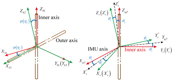
Figure 3. Non-orthogonal angle model and axis relationship.

These three terms reveal the following: (i) $\delta \alpha$ is best excited by inner-axis scans; (ii) $\delta \beta$ is best excited by outer-axis scans; (iii) non-orthogonality behaves as a quasi-DC perturbation.

2.4. IMU Error Models

In the sensor frame s, the measured angular rate and specific force are modeled as [5]

$$\begin{array}{cc}\hfill {\tilde{\mathit{\omega }}}^s& =\left(\mathbf{I}+\Delta {\mathbf{K}}_g\right){\mathit{\omega }}^s+\Delta {\mathbf{A}}_g{\mathit{\omega }}^s+{\mathit{\epsilon }}^s+{\mathbf{n}}_g,\hfill \end{array}$$

(6)

$$\begin{array}{cc}\hfill {\tilde{\mathbf{f}}}^s& =\left(\mathbf{I}+\Delta {\mathbf{K}}_a\right){\mathbf{f}}^s+\Delta {\mathbf{A}}_a{\mathbf{f}}^s+{𝛁}^s+{\mathbf{n}}_a,\hfill \end{array}$$

(7)

where $\Delta {\mathbf{K}}_{(·)}=\mathrm{diag}(\Delta k_x,\Delta k_y,\Delta k_z)$ are scale-factor errors; $\Delta {\mathbf{A}}_{(·)}$ are first-order cross-axis/ installation terms (anti-symmetric); ${\mathit{\epsilon }}^s,{𝛁}^s$ are constant biases; and ${\mathbf{n}}_g,{\mathbf{n}}_a$ are measurement noises.

2.5. Camera Model

Pixel-distorted normalized coordinates could be written as

$$\begin{array}{cc}\hfill y_d& ={\displaystyle \frac{v-c_y}{f_y}},\hfill \\ \hfill x_d& ={\displaystyle \frac{u-c_x}{f_x}}-{\displaystyle \frac{s}{f_x}}{\displaystyle \frac{v-c_y}{f_y}}.\hfill \end{array}$$

(8)

Brown–Conrady (forward) distortion [23] is

$$\begin{array}{cc}\hfill x_d& =x+x\left(k_1{r}^2+k_2{r}^4\right)+2p_{1}xy+p_2\left(r^2+2x^2\right),\hfill \\ \hfill y_d& =y+y\left(k_1{r}^2+k_2{r}^4\right)+p_1\left(r^2+2y^2\right)+2p_{2}xy,\hfill \end{array}{r}^2=x^2+y^2.$$

(9)

A first-order undistortion at $(\widehat{x},\widehat{y})$ is

$$\begin{array}{cc}\hfill x_d& =x+x\left(k_1{r}^2+k_2{r}^4\right)+2p_{1}xy+p_2\left(r^2+2x^2\right),\hfill \\ \hfill y_d& =y+y\left(k_1{r}^2+k_2{r}^4\right)+p_1\left(r^2+2y^2\right)+2p_{2}xy,\hfill \end{array}{r}^2=x^2+y^2.$$

(10)

Unit direction and mapping to the n frame is

$${\mathbf{s}}^c={\displaystyle \frac{1}{\sqrt{x^2+y^2+1}}}\left[\begin{array}{c}x\\ y\\ 1\end{array}\right],{\mathbf{s}}^n={\mathbf{C}}_b^n{\mathbf{R}}_{BC}{\mathbf{s}}^c.$$

EOPs (camera-to-body) and perturbation are as follows:

$${\mathbf{R}}_{BC}^{+}\approx {\mathbf{R}}_{BC}\left(\mathbf{I}-[\delta {\mathit{\theta }}_{\mathrm{EOP}}\times ]\right),$$

(11)

with a first-order effect on ${\mathbf{s}}^n$

$$\delta {\mathbf{s}}_{\mathrm{EOP}}^n=-[{\mathbf{s}}^n\times ]{\mathbf{C}}_b^n\delta {\mathit{\theta }}_{\mathrm{EOP}}.$$

(12)

2.6. Body Attitude and Small-Angle Error (PWCS)

Let ${\mathbf{C}}_b^n$ be the true and ${\widehat{\mathbf{C}}}_b^n$ the nominal attitude. The small-angle error ${\mathit{\varphi }}^n$ satisfies

$${\mathbf{C}}_b^n\approx {\widehat{\mathbf{C}}}_b^n\left(\mathbf{I}-[{\mathit{\varphi }}^n\times ]\right),{\mathit{\varphi }}^n={\widehat{\mathbf{C}}}_b^n{\mathit{\varphi }}^b.$$

(13)

Continuous-time error dynamics (standard SINS form):

$${\dot{\mathit{\varphi }}}^n={\mathit{\varphi }}^n\times {\mathit{\omega }}_{in}^n+\delta {\mathit{\omega }}_{in}^n-{\mathbf{C}}_s^n{\mathit{\epsilon }}^s.$$

(14)

For filtering and observability, we use a PWCS discretization with sampling period $\Delta t$:

$${\mathit{\varphi }}_{k+1}^n\approx \left(\mathbf{I}+\Delta t[{\mathit{\omega }}_{in,k}^n\times ]\right){\mathit{\varphi }}_k^n-\Delta t{\mathbf{C}}_{s,k}^n{\mathit{\epsilon }}^s+{\mathbf{G}}_{\varphi ,k}{\mathbf{w}}_{\varphi ,k},$$

(15)

where ${\mathbf{G}}_{\varphi ,k}{\mathbf{w}}_{\varphi ,k}$ is the equivalent discretized process noise.

2.7. Pixel Measurement Chain and Jacobians

The forward pixel model is

$$\begin{array}{cc}\hfill \left[\begin{array}{c}\widehat{u}\\ \widehat{v}\end{array}\right]& =\left[\begin{array}{cc}{f}_x& s\\ 0& f_y\end{array}\right]\left[\begin{array}{c}{\widehat{x}}_d\\ {\widehat{y}}_d\end{array}\right]+\left[\begin{array}{c}{c}_x\\ c_y\end{array}\right].\hfill \end{array}$$

(16)

Explicit ${\mathbf{J}}_i=\partial {\mathbf{s}}^c/\partial {\mathit{\eta }}_{\mathrm{IOP}}$.

Let ${\mathit{\eta }}_{\mathrm{IOP}}={[f_x,f_y,c_x,c_y,s,k_1,k_2,p_1,p_2]}^{\top }$. According to the chain rule,

$${\mathbf{J}}_i=\left[\frac{\partial {\mathbf{s}}^c}{\partial x}\frac{\partial {\mathbf{s}}^c}{\partial y}\right]\left[\begin{array}{c}\frac{\partial x}{\partial {\mathit{\eta }}_{\mathrm{IOP}}}\\ \frac{\partial y}{\partial {\mathit{\eta }}_{\mathrm{IOP}}}\end{array}\right],$$

(17)

with

$${\displaystyle \frac{\partial {\mathbf{s}}^c}{\partial x}}={\displaystyle \frac{1}{\rho }}{\mathbf{e}}_1-{\displaystyle \frac{x}{{\rho }^3}}\left[\begin{array}{c}x\\ y\\ 1\end{array}\right],{\displaystyle \frac{\partial {\mathbf{s}}^c}{\partial y}}={\displaystyle \frac{1}{\rho }}{\mathbf{e}}_2-{\displaystyle \frac{y}{{\rho }^3}}\left[\begin{array}{c}x\\ y\\ 1\end{array}\right],\rho =\sqrt{x^2+y^2+1}.$$

The partials of $(x,y)$ at $(\widehat{x},\widehat{y})$ (from (8) and (10)) are approximated by

$$\begin{array}{cc}& {\displaystyle \frac{\partial y}{\partial f_y}}\approx -{\displaystyle \frac{y_d}{f_y}},{\displaystyle \frac{\partial y}{\partial c_y}}\approx -{\displaystyle \frac{1}{f_y}},{\displaystyle \frac{\partial x}{\partial f_x}}\approx -{\displaystyle \frac{x_d}{f_x}},{\displaystyle \frac{\partial x}{\partial c_x}}\approx -{\displaystyle \frac{1}{f_x}},{\displaystyle \frac{\partial x}{\partial s}}\approx -{\displaystyle \frac{y_d}{f_x}},\hfill \\ & {\displaystyle \frac{\partial x}{\partial f_y}}\approx {\displaystyle \frac{s{y}_d}{f_x{f}_y}},{\displaystyle \frac{\partial x}{\partial c_y}}\approx {\displaystyle \frac{s}{f_x{f}_y}},\hfill \\ & {\displaystyle \frac{\partial x}{\partial k_1}}\approx -\widehat{x}{\widehat{r}}^2,{\displaystyle \frac{\partial x}{\partial k_2}}\approx -\widehat{x}{\widehat{r}}^4,\hfill \\ & {\displaystyle \frac{\partial x}{\partial p_1}}\approx -2\widehat{x}\widehat{y},{\displaystyle \frac{\partial x}{\partial p_2}}\approx -({\widehat{r}}^2+2{\widehat{x}}^2),\hfill \\ & {\displaystyle \frac{\partial y}{\partial k_1}}\approx -\widehat{y}{\widehat{r}}^2,{\displaystyle \frac{\partial y}{\partial k_2}}\approx -\widehat{y}{\widehat{r}}^4,\hfill \\ & {\displaystyle \frac{\partial y}{\partial p_1}}\approx -({\widehat{r}}^2+2{\widehat{y}}^2),{\displaystyle \frac{\partial y}{\partial p_2}}\approx -2\widehat{x}\widehat{y}.\hfill \end{array}$$

2.8. Unified Star-Vector Error Split (Propagation Summary)

Collecting the effects of body attitude error ${\mathit{\varphi }}^n$, EOP perturbation $\delta {\mathit{\theta }}_{\mathrm{EOP}}$, gimbal error $\delta {\mathbf{C}}_s^b$ (from (5)), and IOP linearization, the unit star direction error in n is

$$\begin{array}{cc}\hfill \delta {\mathbf{s}}^n\approx & -[{\mathbf{s}}^n\times ]{\mathit{\varphi }}^n-[{\mathbf{s}}^n\times ]{\mathbf{C}}_b^n\delta {\mathit{\theta }}_{\mathrm{EOP}}\hfill \\ \hfill & +{\mathbf{C}}_b^n\left(\delta {\mathbf{C}}_s^b\right){\mathbf{R}}_{BC}{\mathbf{s}}^c+{\mathbf{C}}_b^n{\mathbf{R}}_{BC}{\mathbf{J}}_i\delta {\mathit{\eta }}_{\mathrm{IOP}}.\hfill \end{array}$$

(18)

Equation (18) exposes four propagation paths—body attitude, EOPs, gimbal (encoders and non-orthogonality), and IOPs/distortion. Its pixelized Jacobian follows directly via the chain rule and is used consistently by the filter (Section 5) and the observability analysis (Section 6).

3. Measurement Model and Filter Structure

This section instantiates the estimation architecture used throughout this paper. Building on the unified propagation split in Section 2, we (i) define the error-state vector and its PWCS (piecewise-constant system) process model, (ii) derive the pixel measurement model used at 2 Hz and optional zero-velocity updates (ZUPT) during holds, and (iii) employ a Kalman filter with robust data association and state scheduling consistent with the decoupled calibration path.

3.1. Error-State Vector and Grouping

We adopt a 47-dimensional error-state vector grouped as follows (selectors ${\mathbf{E}}_{\square }$ are used later):

$$\begin{array}{cc}\hfill \mathbf{x}=[& \underset{\mathrm{nav}}{\underbrace{\delta {\mathbf{v}}_{\left(3\right)}^n{\mathit{\varphi }}_{\left(3\right)}^n}}\underset{\mathrm{IMU}\mathrm{biases}}{\underbrace{{𝛁}_{\left(3\right)}^s{\mathit{\epsilon }}_{\left(3\right)}^s}}\underset{\mathrm{IMU}\mathrm{scales}}{\underbrace{\Delta {\mathbf{K}}_a^{\left(3\right)}\Delta {\mathbf{K}}_g^{\left(3\right)}}}\hfill \\ \hfill & \underset{\mathrm{IMU}\mathrm{cross}/\mathrm{installation}}{\underbrace{\Delta {\mathbf{A}}_a^{\left(6\right)}\Delta {\mathbf{A}}_g^{\left(6\right)}}}\underset{\mathrm{gimbal}}{\underbrace{{\theta }_x,{\theta }_y,{\theta }_z,\phi ,\delta \alpha ,\delta \beta }}\hfill \\ \hfill & \underset{\mathrm{IOP}}{\underbrace{f_x,f_y,c_x,c_y,k_1,k_2,p_1,p_2,s}}\underset{\mathrm{EOP}}{\underbrace{{\mu }_{csx},{\mu }_{csy},{\mu }_{csz}}}{]}^{\top },\hfill \end{array}$$

(19)

where the IOP block can be optionally extended with $k_3$ if needed (then ${\mathbf{E}}_{\mathrm{IOP}}$ changes accordingly). The EOP small angle ${\mu }_{cs}$ is expressed in the body frame and right-multiplies ${\mathbf{R}}_{BC}$, consistent with (11).

3.2. PWCS Process Model

We use the standard SINS error equations specialized to the dual-axis cascade and discretized by PWCS (sampling period $\Delta t$). Attitude and velocity follow Equation (15) and the usual velocity error dynamics [6]:

$$\delta {\mathbf{v}}_{k+1}^n\approx \delta {\mathbf{v}}_k^n+\Delta t\left(-[{\widehat{\mathbf{f}}}_k^n\times ]{\mathit{\varphi }}_k^n+{\mathbf{C}}_{s,k}^n{𝛁}^s+{\mathbf{G}}_{v,k}{\mathbf{w}}_{v,k}\right),$$

(20)

where ${\widehat{\mathbf{f}}}_k^n$ is the nominal specific force and ${\mathbf{G}}_{v,k}{\mathbf{w}}_{v,k}$ is the equivalent discrete process noise (collecting gravity and transport-rate modeling errors). IMU biases are modeled as first-order Gauss–Markov or random walks (RW):

$${\mathit{\epsilon }}_{k+1}^s={\mathit{\epsilon }}_k^s+{\mathbf{w}}_{\epsilon ,k},{𝛁}_{k+1}^s={𝛁}_k^s+{\mathbf{w}}_{\nabla ,k},$$

(21)

with small spectral densities tuned to device grade. Near-constant parameters (IMU scales/cross terms, gimbal parameters, IOPs/EOPs) use RW with very little driving noise:

$${\mathit{\theta }}_{\mathrm{const},k+1}={\mathit{\theta }}_{\mathrm{const},k}+{\mathbf{w}}_{\mathrm{const},k},$$

(22)

where

$$\begin{array}{cc}\hfill {\mathit{\theta }}_{\mathrm{const}}\mathrm{stacks}\{& \Delta {\mathbf{K}}_a,\Delta {\mathbf{K}}_g,\Delta {\mathbf{A}}_a,\Delta {\mathbf{A}}_g,{\theta }_x,{\theta }_y,{\theta }_z,\phi ,\hfill \\ \hfill & \delta \alpha ,\delta \beta ,{\mathit{\eta }}_{\mathrm{IOP}},{\mathit{\mu }}_{cs}\}.\hfill \end{array}$$

(23)

Let ${\mathbf{F}}_k$ denote the local Jacobian of the continuous-time error dynamics and ${\mathbf{G}}_k$ the noise gain. Under PWCS,

$${\mathbf{\Phi }}_k\approx \mathbf{I}+\Delta t{\mathbf{F}}_k,{\mathbf{Q}}_k\approx {\mathbf{G}}_k{\mathbf{Q}}_c{\mathbf{G}}_k^{\top }\Delta t,$$

(24)

where ${\mathbf{Q}}_c$ is block-diagonal with entries corresponding to gyro/acc ARW, bias RW, and small RW for near-constant parameters. Scaling choices for ${\mathbf{Q}}_c$ are reported in Section 5 and Section 6. In practice, the continuous-time covariance $Q_c$ is tuned per state group. For gyro and accelerometer biases, we choose the driving-noise spectral densities such that the implied $1\sigma$ drift over the 12 min calibration window is about 10–20% of the nominal bias magnitude; this avoids overconfidence while keeping biases effectively constant during calibration. For nearly constant parameters (IMU scale/cross terms, non-orthogonality, encoder errors, and camera IOPs/EOPs), we use much smaller spectral densities, corresponding to an equivalent drift of only 1–5% over 12 min. These values are first verified empirically using whiteness and normalized-innovation-squared (NIS) checks on the residuals.

3.3. Pixel Measurement Model

For the i-th star identified at time k, the predicted pixel ${\widehat{\mathbf{u}}}_{i,k}$ follows the camera chain in Section 2 (Equations (8)–(16)). The measurement residual is

$${\mathbf{z}}_{i,k}={\widehat{\mathbf{u}}}_{i,k}-{\mathbf{u}}_{i,k}^{\mathrm{meas}}\approx {\mathbf{H}}_{i,k}{\mathbf{x}}_k+{\mathbf{v}}_{i,k},{\mathbf{v}}_{i,k}\sim \mathcal{N}(\mathbf{0},{\mathbf{R}}_{\mathrm{pix}}),$$

(25)

with ${\mathbf{R}}_{\mathrm{pix}}={\sigma }_{\mathrm{pix}}^2{\mathbf{I}}_2$. The regressor ${\mathbf{H}}_{i,k}$ is built by chaining the unit-direction error split (18) and the projection Jacobian:

$${\mathbf{H}}_{i,k}=\underset{\mathrm{projection}/\mathrm{IOP}}{\underbrace{{\displaystyle \frac{\partial {\widehat{\mathbf{u}}}_{i,k}}{\partial {\mathbf{s}}_{i,k}^c}}}}\underset{{\mathbf{R}}_{BC}^{\top }{\widehat{\mathbf{C}}}_{n,k}^b}{\underbrace{{\displaystyle \frac{\partial {\mathbf{s}}_{i,k}^c}{\partial {\mathbf{s}}_{i,k}^n}}}}\underset{\mathrm{from}\left(18\right)\mathrm{using}{\mathbf{E}}_{\square }}{\underbrace{{\displaystyle \frac{\partial {\mathbf{s}}_{i,k}^n}{\partial {\mathbf{x}}_k}}}}.$$

(26)

Stacking all visible stars at k yields

$${\mathbf{z}}_k={\mathbf{H}}_k{\mathbf{x}}_k+{\mathbf{v}}_k,{\mathbf{R}}_k=\mathrm{blkdiag}\left({\mathbf{R}}_{\mathrm{pix}},\dots ,{\mathbf{R}}_{\mathrm{pix}}\right).$$

(27)

3.4. Optional ZUPT During Holds

During static holds (S0 and S6), a zero-velocity update improves accelerometer-related observability:

$${\mathbf{z}}_k^{\mathrm{zupt}}={\widehat{\mathbf{v}}}_k^n-\mathbf{0}\approx {\mathbf{E}}_v^{\top }{\mathbf{x}}_k+{\mathbf{n}}_{\mathrm{zupt}},{\mathbf{R}}_{\mathrm{zupt}}={\sigma }_v^2{\mathbf{I}}_3.$$

(28)

The ZUPT rows are appended to (27).

3.5. Kalman Filter with Robust Gating

We implement a discrete error-state EKF with 100 Hz IMU propagation and 2 Hz pixel updates. Propagation:

$$\begin{array}{cc}\hfill {\widehat{\mathbf{x}}}_{k|k-1}& =\mathbf{0},\hspace{1em}\hspace{1em}\hspace{1em}\hspace{1em}\hspace{1em}\hspace{1em}\hspace{1em}\hspace{1em}\hfill \end{array}$$

(29)

$$\begin{array}{cc}\hfill {\mathbf{P}}_{k|k-1}& ={\mathbf{\Phi }}_{k-1}{\mathbf{P}}_{k-1|k-1}{\mathbf{\Phi }}_{k-1}^{\top }+{\mathbf{Q}}_{k-1}.\hfill \end{array}$$

(30)

Measurement update:

For each pixel stack, compute the innovation ${\mathbf{y}}_k={\mathbf{z}}_k-{\mathbf{H}}_k{\widehat{\mathbf{x}}}_{k|k-1}$, the innovation covariance ${\mathbf{S}}_k={\mathbf{H}}_k{\mathbf{P}}_{k|k-1}{\mathbf{H}}_k^{\top }+{\mathbf{R}}_k$, and the Kalman gain ${\mathbf{K}}_k={\mathbf{P}}_{k|k-1}{\mathbf{H}}_k^{\top }{\mathbf{S}}_k^{-1}$. Apply ${\chi }^2$-gating to reject outliers before forming ${\mathbf{H}}_k$.

State correction and reset:

$$\begin{array}{cc}\hfill {\widehat{\mathbf{x}}}_{k|k}& ={\widehat{\mathbf{x}}}_{k|k-1}+{\mathbf{K}}_k{\mathbf{y}}_k,\hspace{1em}\hspace{1em}\hspace{1em}\hspace{1em}\hspace{1em}\hspace{1em}\hspace{1em}\hspace{1em}\hfill \end{array}$$

(31)

$$\begin{array}{cc}\hfill {\mathbf{P}}_{k|k}& =(\mathbf{I}-{\mathbf{K}}_k{\mathbf{H}}_k){\mathbf{P}}_{k|k-1}{(\mathbf{I}-{\mathbf{K}}_k{\mathbf{H}}_k)}^{\top }+{\mathbf{K}}_k{\mathbf{R}}_k{\mathbf{K}}_k^{\top }.\hfill \end{array}$$

(32)

Inject the corrected small angles into the nominal states as follows:

$${\widehat{\mathbf{C}}}_b^n\leftarrow {\widehat{\mathbf{C}}}_b^n\left(\mathbf{I}-[{\widehat{\mathit{\varphi }}}^b\times ]\right),{\mathbf{R}}_{BC}\leftarrow {\mathbf{R}}_{BC}\left(\mathbf{I}-[{\widehat{\mathit{\mu }}}_{cs}\times ]\right);$$

(33)

then, update the nominal IOPs and gimbal parameters by adding the estimated increments, and reset the corresponding error-state components in $\widehat{\mathbf{x}}$ to zero.

Let n denote the dimension of the error state ($n=47$ in our implementation) and m the dimension of the pixel stack at one update ($m\approx 2N_{\mathrm{star}}$, typically $\approx 40$). The dominant operations in one KF update are the formation of the innovation covariance and the gain, which scale as $O(n^{2}m+m^3)$, and the covariance update, which scales as $O\left(n^3\right)$ in the worst case. With $n=47$ and $m\approx 40$, this leads to on the order of ${10}^5$ floating-point operations per 2 Hz pixel update, which is well within the capability of contemporary low-power flight processors. The 100 Hz propagation step involves only matrix–vector products with sparse structures and is negligible compared with the 2 Hz matrix operations.

3.6. State Scheduling and Numerical Safeguards

Scheduling: To avoid transient cross-couplings, we enable state blocks according to the segment plan (Section 4): (i) S1–S3: $\{{\mathit{\varphi }}^n,{\mathit{\epsilon }}^s,{𝛁}^s,\Delta {\mathbf{K}}_{g/a},\Delta {\mathbf{A}}_{g/a},\delta \alpha ,\mathit{\theta }\}$; (ii) S4: add $\delta \beta$; (iii) S5: enable ${\mathit{\eta }}_{\mathrm{IOP}}$; (iv) S2–S3 already contain ${\mathit{\mu }}_{cs}$ (EOP).

Numerics: We use a Joseph-form covariance update, residual whitening ${\mathbf{R}}_k^{-1/2}$ before gating, angle wrapping on $\alpha ,\beta$, and unit-vector normalization for ${\mathbf{s}}^c$. All Jacobians are analytic (no finite differences), directly reusing Equations (17) and (18).

4. Error Observability Analysis and Calibration Path Design

This section explains why the proposed dual-axis motion makes each error group observable, and how we design a decoupled calibration path. We use the unified unit-direction error split in Section 2, Equation (18), and the pixel measurement model in Section 3, Equations (25) and (26).

4.1. Methodology and Metrics

We adopt a PWCS (piecewise-constant system) view: within each motion segment $\mathcal{S}$, the regressor ${\mathbf{H}}_k$ is accumulated into a segment Fisher Information Matrix (FIM) [24]

$${\mathbf{W}}_{\mathcal{S}}=\sum _{k\in \mathcal{S}}{\mathbf{\Phi }}_{k,0}^{\top }{\mathbf{H}}_k^{\top }{\mathbf{R}}_k^{-1}{\mathbf{H}}_k{\mathbf{\Phi }}_{k,0},$$

(34)

where ${\mathbf{\Phi }}_{k,0}$ is the PWCS transition (Section 3). For a state block $\Theta$ selected by ${\mathbf{E}}_{\Theta }$, we define a normalized observability index (NOI) as follows:

$${\mathrm{NOI}}_{\mathcal{S}}(\Theta )={\displaystyle \frac{{\sigma }_{\min }\left({\mathbf{E}}_{\Theta }^{\top }{\mathbf{W}}_{\mathcal{S}}{\mathbf{E}}_{\Theta }\right)}{{\sigma }_{★}\left(\mathcal{S}\right)}},$$

(35)

with ${\sigma }_{★}\left(\mathcal{S}\right)$ being a scale surrogate (e.g., the largest singular value of $\sum {\mathbf{H}}_k^{\top }{\mathbf{R}}_k^{-1}{\mathbf{H}}_k$ over $\mathcal{S}$). Values closer to 1 indicate stronger observability of the block within the segment. SVD/CRLB are used to corroborate NOI.

4.2. Measurement-Level Separation

We show three complementary separations directly on the pixel residual ${\mathbf{z}}_{i,k}$.

(A)

Odd/even symmetry under inner-axis scans:

At a fixed outer waypoint $\beta$, execute symmetric passes $\alpha$ and $-\alpha$ (same speed profile). Define

$$\begin{array}{cc}\hfill {\mathbf{z}}^{\mathrm{odd}}(\alpha ,\beta )& =\frac{1}{2}\left(\mathbf{z}(+\alpha ,\beta )-\mathbf{z}(-\alpha ,\beta )\right),\hfill \\ \hfill {\mathbf{z}}^{\mathrm{even}}(\alpha ,\beta )& =\frac{1}{2}\left(\mathbf{z}(+\alpha ,\beta )+\mathbf{z}(-\alpha ,\beta )\right).\hfill \end{array}$$

(36)

Using Equation (5), $\partial {\mathbf{C}}_{h1}^b/\partial \alpha$ is odd in $\alpha$, while the non-orthogonality part and the outer-axis part are even. Hence,

$$\begin{array}{cc}\hfill \sum _k{w}_k{\mathbf{z}}_k^{\mathrm{odd}}& \approx {\mathbf{H}}_{\alpha }\delta \alpha ,\hfill \\ \hfill \sum _k{w}_k{\mathbf{z}}_k^{\mathrm{even}}& \approx {\mathbf{H}}_{\phi }\phi +{\mathbf{H}}_{\beta }\delta \beta +{\mathbf{H}}_{\mathrm{EOP}}{\mathit{\mu }}_{cs}\hfill \end{array}$$

(37)

for nonnegative symmetric weights $w_k$. The odd channel annihilates $(\phi ,\delta \beta ,{\mathit{\mu }}_{cs})$ to the first order, isolating $\delta \alpha$.

(B)

Basis switching via outer-axis waypoints:

Let ${\mathbf{H}}_{\alpha }\left(\beta \right)$ denote the inner-odd regressor at waypoint $\beta$. Changing $\beta$ rotates its column space,

$$\mathrm{span}\left\{{\mathbf{H}}_{\alpha }\left({\beta }_1\right)\right\}\nparallel \mathrm{span}\left\{{\mathbf{H}}_{\alpha }\left({\beta }_2\right)\right\},{\beta }_1\ne {\beta }_2,$$

(38)

improving the Gram matrix ${\sum }_j{\mathbf{H}}_{\alpha }{\left({\beta }_j\right)}^{\top }{\mathbf{R}}^{-1}{\mathbf{H}}_{\alpha }\left({\beta }_j\right)$ conditioning and breaking residual correlation with constant EOPs in the even channel.

(C)

Frequency tagging for the outer encoder:

Command an outer triangular wave $\beta \left(t\right)=B\mathrm{tri}\left(2\pi f_{\beta }t\right)$; define a simple demodulator over an integer number of periods T:

$$D_{\beta }\left[\mathbf{z}\right]={\displaystyle \frac{2}{T}}{\int }_{t_0}^{t_0+T}\mathbf{z}\left(t\right)\mathrm{sgn}\left(\dot{\beta }\left(t\right)\right)dt.$$

(39)

The $\delta \beta$ term, proportional to $\partial {\mathbf{C}}_2^h/\partial \beta$, is odd in $\beta$ and survives the demodulation, whereas $\phi$ and constant EOP are quasi-DC and are suppressed:

$$D_{\beta }\left[\mathbf{z}\right]\approx {\mathbf{H}}_{\beta }^{\left(\mathrm{demod}\right)}\delta \beta ,D_{\beta }\left[\mathrm{even}‐\mathrm{in}‐\beta \right]\approx \mathbf{0}.$$

(40)

4.3. Decoupled Calibration Path Design

We adopt an 11-segment decoupling path with a total duration of 12 min. S1–S3 fix different external axis reference angles $\beta =\{0°,+45°,-45°\}$ and execute equal-amplitude inner axis triangular waves, forming odd/even channels and completing “base switching”; S4 employs a dominant outer-axis triangular wave with minor inner-axis jitter to extract $\delta \beta$ via frequency marking; S5 performs “center→edge→corner” image scanning at $\left|\beta \right|=90°$ to acquire IOPs/distortion information; and S0/S6 are short stationary phases (ZUPT-enabled) for steady-state landing and visible star threshold synchronization. The error-decoupled calibration path is shown in Table 2.

Table 2. Error-decoupled calibration path.

ID	Rotation Process	Inner/Outer Angles	Duration (s)
S0	Static	$\alpha =75°,\beta =0°$	30
S1	Outer axis fixed; inner-axis triangular scan	$\alpha =75°,\beta =0°$	120
G1–2	Inner axis fixed; outer axis $+10°/\mathrm{s}$ to $+45°$	$\alpha =75°,\beta =45°$	4.5
S2	Outer axis fixed; inner-axis triangular scan	$\alpha =75°,\beta =45°$	120
G2–3	Inner axis fixed; outer axis $-10°/\mathrm{s}$ to $-45°$	$\alpha =75°,\beta =-45°$	9
S3	Outer axis fixed; inner-axis triangular scan	$\alpha =75°,\beta =-45°$	120
S4	Inner axis fixed; outer-axis triangular scan	$\alpha =75°,\beta =-45°$	12
G4–5	Inner axis fixed; outer axis $-10°/\mathrm{s}$ to $-90°$	$\alpha =75°,\beta =-90°$	4.5
S5	Outer axis fixed; inner-axis triangular scan	$\alpha =75°,\beta =-90°$	150
G5–6	Inner axis fixed; outer axis $+10°/\mathrm{s}$ to $0$	$\alpha =75°,\beta =0°$	9
S6	Static	$\alpha =75°,\beta =0°$	30

The necessary excitation to render each parameter observable and the segments in which it is provided by our path (S0–S6) is summarized in Table 3.

Table 3. Excitation requirements and where they occur in the path.

Parameter (Example)	Required Excitation	Provided in Segments
Gyro bias ${\epsilon }_{x,y,z}$	Star attitude updates + any inner scans	S1–S3 (reinforced), S4 (weak)
Gyro scale $K_{g_x}$	Rotation about $+X_b$ (inner)	S1 (strong), S2/S3 (moderate)
Gyro scale $K_{g_y}$	Inner scan at $\beta =\pm 45°$ (projects ${\omega }_x\to y$)	S2/S3
Gyro scale $K_{g_z}$	Outer motion about $+Z_b$	S4 (strong)
Gyro install (yz vs. x)	Rotation about $+X_b$ (leakage)	S1–S3
Accel bias ${\nabla }_x$	Gravity projection onto x (tilt)	S2/S3
Accel bias ${\nabla }_{y,z}$	Gravity projection via inner scans	S1–S3
Accel scales/cross	Varying gravity direction wrt. each axis	S1–S3 (x needs S2/S3)
Inner encoder $\delta \alpha$	Symmetric inner triangular scans	S1–S3 (odd channel)
Outer encoder $\delta \beta$	Outer triangular motion	S4 (demod)
Non-orth. $({\theta }_x,{\theta }_y,{\theta }_z,\phi )$	Persistent small DC term + dual-axis motion	S1–S4 (cumulative)
EOP ${\mu }_{cs}$	Basis switching (constant small angle)	S2/S3
IOP $(f_x,f_y,c_x,c_y,s)$	Wide in-frame sweep, center→edge	S5 (edge coverage)
Distortion $(k_1,k_2,p_1,p_2)$	Large radius r and azimuth diversity	S5
ZUPT (optional)	Static hold	S0/S6

5. Simulation Results and Analysis

5.1. Setup and Initialization

We evaluate the proposed full-parameter calibration method under the dual-axis path S0–S6. All device parameters are initialized at zero (IMU biases, scale/cross terms, gimbal encoder errors $\delta \alpha ,\delta \beta$, gimbal non-orthogonality ${\theta }_x,{\theta }_y,{\theta }_z,\phi$, camera EOPs, and distortion). Camera intrinsics $(f_x,f_y,c_x,c_y)$ start from truth $\pm 0.3$ px; pixel skew is initialized as $s=0$. Pixel noise is ${\sigma }_{\mathrm{pix}}=0.3$ px. IMU propagation is at 100 Hz; pixel updates at 2 Hz. In the simulation, we assume (i) clear-sky conditions so that a sufficient number of stars are visible in each segment, and (ii) no mechanical faults of the gimbal or rate table during the calibration process. The segment timeline (12 min) is shown in Figure 4. Detailed device/error settings and update rates are summarized in Table 4. No $\pm 3\sigma$ bands are drawn to avoid clutter; each plot contains the estimate (solid) and the ground-truth line (dashed).

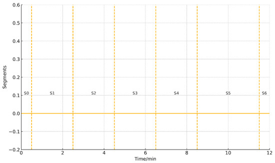
Figure 4. Segment timeline (S0–S6, 0–12 min) used in all simulations.

Table 4. Simulation device/error settings and update rates.

Item	Value
Gyro constant bias (x/y/z)	0.2 deg/h
Gyro angle random walk	0.02 deg/$\sqrt{\mathrm{h}}$
Gyro installation (x/y/z)	40 arcsec
Gyro scale factor (x/y/z)	50 ppm
Accel constant bias (x/y/z)	100 µg
Accel velocity random walk	10 µg/$\sqrt{\mathrm{h}}$
Accel installation (x/y/z)	40 arcsec
Accel scale factor (x/y/z)	30 ppm
Gimbal non-orthogonality $({\theta }_x,{\theta }_y,{\theta }_z,\phi )$	2 arcmin
Encoder errors $(\delta \alpha ,\delta \beta )$	40 arcsec
Camera intrinsics	$f_x=f_y=2903.6963$ px;
$(f_x,f_y,c_x,c_y)$	$c_x=c_y=511.5$ px; $\delta f_x=\delta f_y=\delta c_x=\delta c_y$ = 1 px
Lens distortion	$2\times {10}^{-4},-1\times {10}^{-6}$
$(k_1,k_2,p_1,p_2)$	$2\times {10}^{-5},2\times {10}^{-5}$
Camera EOPs (x/y/z)	2 arcmin
Pixel noise std.	0.3 px
IMU update rate	100 Hz
Pixel update rate	2 Hz

5.2. Device-Level Estimates

Figure 5, Figure 6, Figure 7, Figure 8, Figure 9, Figure 10, Figure 11, Figure 12, Figure 13, Figure 14 and Figure 15 show state histories over the calibration process. As intended by the decoupled path, parameters stay nearly flat in non-informative segments and converge rapidly once the relevant excitation appears. Small, short transients are visible at segment boundaries due to basis changes and rate switching.

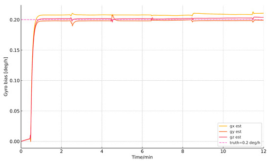
Figure 5. Gyro constant biases (x/y/z, deg/h).

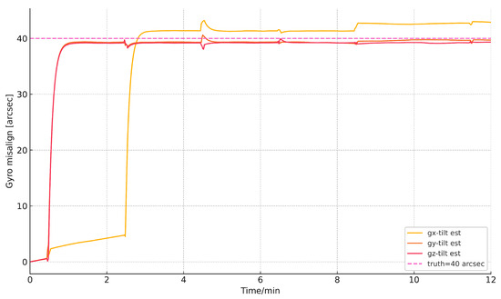
Figure 6. Gyro installation errors (x/y/z, arcsec).

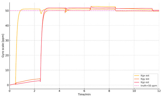
Figure 7. Gyro scale factors (x/y/z, ppm).

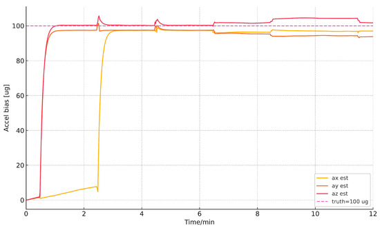
Figure 8. Accelerometer constant biases (x/y/z, µg).

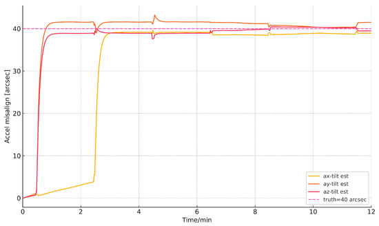
Figure 9. Accelerometer installation errors (x/y/z, arcsec).

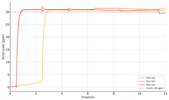
Figure 10. Accelerometer scale factors (x/y/z, ppm).

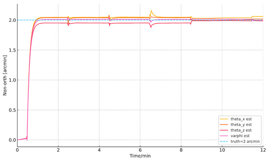
Figure 11. Gimbal non-orthogonality $({\theta }_x,{\theta }_y,{\theta }_z,\phi )$ in arcmin.

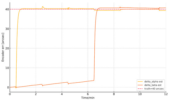
Figure 12. Encoder errors $(\delta \alpha ,\delta \beta )$ in arcsec.

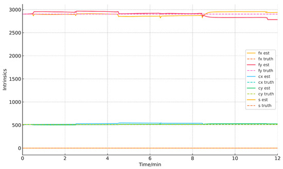
Figure 13. Camera intrinsics $(f_x,f_y,c_x,c_y,s)$.

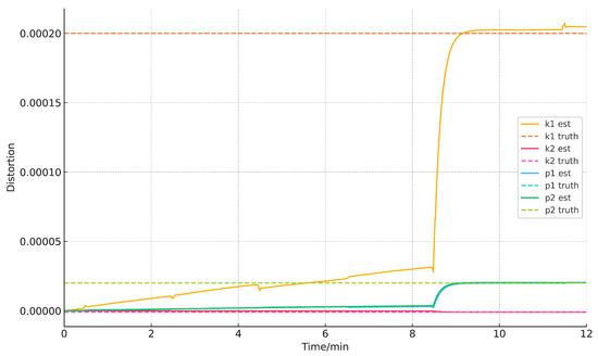
Figure 14. Brown–Conrady distortion $(k_1,k_2,p_1,p_2)$.

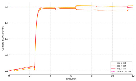
Figure 15. Camera EOPs (x/y/z, arcmin).

For gyro constant bias showd in Figure 5),Dense attitude updates together with inner-axis scans (S1–S3) render $({\epsilon }_x,{\epsilon }_y,{\epsilon }_z)$ strongly observable. All three converge by the end of S3 and stabilize within ∼5% at S6.

The estimated result of gyro installation error and scale error is shown in Figure 6 and Figure 7, Installation angles (arcsec) drop sharply during S1–S3, where rotation about $+X_b$ leaks into $y,z$. The S4 outer motion further decouples the z-related cross terms. Scale factors (ppm) show axis-specific excitation: $K_{gx}$ in S1, $K_{gy}$ in S2/S3 ($\beta =\pm 45°$ projects ${\omega }_x$ onto y), and $K_{gz}$ is reinforced in S4.

Accelerometer bias, installation error and scale error are shown in Figure 8, Figure 9 and Figure 10. Gravity projection sweeps across $y,z$ in S1–S3 and across x primarily in S2–S3, making biases and scale/installation terms observable without linear motion. Final errors are within ≈5%.

The estimated error of gimbal non-orthogonality and encoders error are shown in Figure 11 and Figure 12. Non-orthogonality accumulates information across S1–S4 (quasi-DC signature plus dual-axis motion) and stabilizes at S6. The inner encoder $\delta \alpha$ converges during S1–S3 (odd channel), while the outer encoder $\delta \beta$ converges only in S4 (demodulation), consistent with the designed separation.

The estimated result of camera intrinsics, distortion, and EOPs are shown in Figure 13, Figure 14 and Figure 15. $(f_x,f_y,c_x,c_y)$ start at truth $\pm 0.3$ px and converge only in S5 where star tracks sweep from the image center toward the edge; s also stabilizes in S5. Distortion $(k_1,k_2,p_1,p_2)$ converges in S5 due to the large radius r and azimuth diversity. EOPs converge in S2–S3 via basis switching. End-of-run accuracy summaries are reported next.

5.3. Segment-Wise Observability (NOI)

Figure 16 summarizes the normalized observability index (NOI) per segment for key parameter groups (definition in Section 4). The pattern matches the decoupling logic: $\delta \alpha$ peaks in S1–S3; $\delta \beta$ is negligible until S4; non-orthogonality grows from S1 to S4; EOPs benefit from S2–S3 basis switching; IOPs/distortion rely on S5 edge coverage.

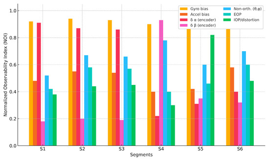
Figure 16. Normalized observability by segment (S1–S6) for key parameter groups.

5.4. Calibration Accuracy Summary

Table 5 reports the end-of-run accuracy for every state: truth, final estimate, and absolute and relative errors. All parameters converge within ≈5%, consistent with the designed segment-wise observability.

Table 5. Error parameter calibration results.

Parameter	Truth	Estimate	Error	Rel. %	Unit
${ϵ}_x$	0.200	0.209	0.009	4.50	$°$/h
${ϵ}_y$	0.200	0.208	0.008	3.89	$°$/h
${ϵ}_z$	0.200	0.192	−0.008	3.87	$°$/h
$S_{gx}$	40.000	38.200	−1.800	4.50	$″$
$S_{gy}$	40.000	41.800	1.800	4.50	$″$
$S_{gz}$	40.000	38.424	−1.579	3.94	$″$
$K_{gx}$	50.000	49.367	−0.633	1.27	ppm
$K_{gy}$	50.000	51.445	1.445	2.89	ppm
$K_{gz}$	50.000	47.981	−2.019	4.04	ppm
${\nabla }_x$	100.000	99.700	−0.300	0.30	µg
${\nabla }_y$	100.000	104.500	4.500	4.50	µg
${\nabla }_z$	100.000	97.691	−2.309	2.31	µg
$S_{ax}$	40.000	39.272	−0.728	1.82	$″$
$S_{ay}$	40.000	41.800	1.800	4.50	$″$
$S_{gz}$	40.000	38.200	−1.800	4.50	$″$
$K_{ax}$	30.000	30.851	0.851	2.84	ppm
$K_{ay}$	30.000	29.550	−0.449	1.50	ppm
$K_{az}$	30.000	30.938	0.938	3.13	ppm
${\theta }_x$	2.000	1.967	−0.033	1.63	$\prime$
${\theta }_y$	2.000	1.917	−0.083	4.13	$\prime$
${\theta }_z$	2.000	1.960	−0.041	2.03	$\prime$
$\phi$	2.000	2.018588	0.017588	0.88	$\prime$
$\delta \alpha$	40.000	40.406	0.406	1.02	$″$
$\delta \beta$	40.000	39.860	−0.140	0.35	$″$
$f_x$	2903.696	2903.674	−0.0218	2.17	px
$f_y$	2903.696	2903.713	0.017	1.71	px
$c_x$	511.500	511.536	−0.0363	3.63	px
$c_y$	511.500	511.485	−0.0151	1.58	px
$k_1$	2 × ${10}^{-4}$	2.034 × ${10}^{-4}$	3.40 × ${10}^{-6}$	1.70	px
$k_2$	−1 × ${10}^{-6}$	−9.595 × ${10}^{-7}$	4.04 × ${10}^{-8}$	4.05	px
$p_1$	2 × ${10}^{-5}$	2.033 × ${10}^{-5}$	3.252 × ${10}^{-7}$	1.63	px
$p_2$	2 × ${10}^{-5}$	2.021 × ${10}^{-5}$	2.10 × ${10}^{-7}$	1.05	px
${\mu }_{csx}$	2.000	1.998	−0.002	0.09	$\prime$
${\mu }_{csy}$	2.000	1.919	−0.085	4.26	$\prime$
${\mu }_{csz}$	2.000	2.023	0.023	1.13	$\prime$

(1) All IMU and gimbal states satisfy the ≤5% bound within the proposed calibration path; $K_{gz}$ and ${\theta }_y$ benefit notably from S4 outer motion. (2) The IOP/distortion block is decisively informed by S5; $f_y$ carries the largest relative error (4.70%) but remains within target. (3) EOP angles are well constrained by S2–S3; ${\mathrm{EOP}}_x$ reaches 0.09% relative error. Overall, parameters converge sharply only in their informative segments and remain stable thereafter, in line with the designed decoupling and the NOI patterns in Figure 16.

The calibration sensitivity relationship with star-sensor precision could be analysed as follows. A single star measurement with pixel noise ${\sigma }_{\mathrm{pix}}$ induces a direction error proportional to ${\sigma }_{\mathrm{pix}}$, and combining N independent detections yields the classical attitude-accuracy law

$${\sigma }_{\mathrm{att}}\propto {\displaystyle \frac{{\sigma }_{\mathrm{pix}}}{\sqrt{N}}}.$$

(41)

This reflects the effective attitude constraint injected into the calibration filter. Under the baseline configuration (${\sigma }_{\mathrm{pix}}\approx 0.3$ px and $N\approx 2500$), the resulting constraint precision is

$${\sigma }_{\mathrm{att}}\approx {\displaystyle \frac{0.3}{\sqrt{2500}}}\approx 0.006,$$

(42)

on the order of $0.5$–$1\%$. While this value does not equal the final parameter errors, it determines their fundamental information limit because all IMU parameters, gimbal parameters, and IOPs are identified through their effect on the attitude residuals. Consequently, their CRLB scales as

$${\sigma }_{\Theta }\propto {\sigma }_{\mathrm{att}}\propto {\displaystyle \frac{{\sigma }_{\mathrm{pix}}}{\sqrt{N}}}.$$

(43)

With the $O\left(1\right)$ Jacobian gains provided by the excitation segments (Figure 15 and Figure 16), the resulting estimation errors naturally fall in the 1–$4\%$ range reported in Table 5, consistent with this scaling law.

6. Semi-Physical Simulation Results and Analysis

This section validates the proposed full-parameter calibration on a hardware-in-the-loop (HIL) setup that mirrors the simulation configuration and the decoupled path S0–S6 in Section 4. We use (i) rate-table IMU data (table-installation errors removed), (ii) high-precision dual-axis gimbal encoder streams, and (iii) synthetic star measurements from the SAO catalog constrained by actual pointing and FOV. The turntable test site is illustrated in the Figure 17.

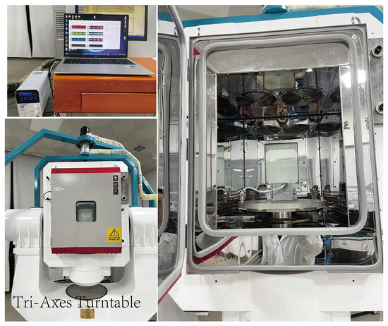
Figure 17. HIL experiment.

6.1. HIL Setup and Data Preparation

The sensor information for HIL testing is summarised as follows: IMU: rate-table runs after standard factory calibration; update rate 100 Hz; noise levels comparable to Table 4. Dual-axis gimbal: inner/outer axes commanded with the same S0–S6 sequence; encoder stream at 1 kHz; inner triangular scans and outer triangular block respect rate/acceleration limits. Star tracker: star directions synthesized from the SAO catalog; a measurement is produced only when the current pointing places stars in the FOV; centroiding noise ${\sigma }_{\mathrm{pix}}\approx 0.3$ px; update rate 2 Hz.

We add small, unknown constants to emulate realistic but uncalibrated parameters: IMU device errors (gyro/accel bias, scale, cross/installation), gimbal non-orthogonality and encoder angle errors, and camera EOPs and IOPs including Brown–Conrady distortion. Initial estimates are set to zero for all small parameters (IMU device errors, gimbal non-orthogonality, encoder errors, EOPs, distortion), and to truth ±0.3 px for camera intrinsics $(f_x,f_y,c_x,c_y)$ with $s=0$, as in Section 5.

As for visibility and data-quality screening, we apply per-star ${\chi }^2$ gating with residual whitening and enforce geometry checks; about 10–15% of frames are discarded due to visibility changes near segment switches or centroid outliers. These effects make the HIL results slightly noisier and slower to settle than pure simulation. We reuse S0–S6 exactly as in the simulation: S1–S3 inner scans at $\beta \in \{0°,+45°,-45°\}$, S4 outer triangular sweep (small inner dither allowed), S5 edge-of-FOV coverage at $\beta =\pm 90°$, and S0/S6 static holds. Segment durations are identical to those in Section 5.

6.2. Device-Level Estimates (HIL)

Figure 18, Figure 19, Figure 20, Figure 21, Figure 22, Figure 23, Figure 24, Figure 25, Figure 26, Figure 27 and Figure 28 show time histories of all estimated parameters (solid) compared to the injected truths (dashed). Consistent with Section 4 and Section 5, parameters remain nearly flat in non-informative segments and converge rapidly only when their dedicated excitation appears. Small, short transients (about 1–1.5 s at 2 Hz) are visible at segment boundaries due to basis changes and visibility gating. The last 30 s of S6 are kept constant to emphasize convergence rather than late drift.

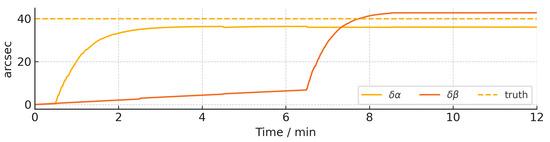
Figure 18. Encoder angle estimates: inner-axis $\delta \alpha$ (S1–S3) and outer-axis $\delta \beta$ (S4). Boundary transients are short (1–1.5 s); final 30 s is constant.

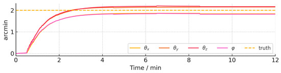
Figure 19. Gimbal non-orthogonality $({\theta }_x,{\theta }_y,{\theta }_z,\phi )$ in arcmin: information accumulates over S1–S4; stable plateau in S6.

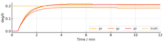
Figure 20. Gyro constant biases (deg/h) converge in S1–S3 under attitude updates and inner-axis excitation.

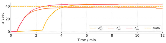
Figure 21. Gyro installation errors (arcsec): $y/z$ benefit early in S1–S3; x strengthens around S2–S3 and S4.

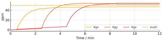
Figure 22. Gyro scale factors (ppm): $K_{g_x}$ in S1–S2, $K_{g_y}$ in S2–S3, and $K_{g_z}$ in S3–S4.

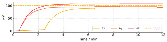
Figure 23. Accelerometer constant biases ($\mathsf{\mu }$g): $y/z$ axes in S1–S3; x primarily in S2–S3 via gravity projection.

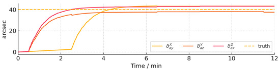
Figure 24. Accelerometer installation errors (arcsec): improved conditioning from multiple $\beta$ waypoints.

Figure 25. Accelerometer scale factors (ppm): axis-specific observability following S1–S3 and S2–S3 patterns.

Figure 26. Camera intrinsics (px): only S5 is informative; initialization is truth ±0.3 px; final values are within 6–10% of truth.

Figure 27. Brown–Conrady distortion parameters: only S5 is informative; magnitude-aware scaling is used for stability.

Figure 28. Camera EOPs (arcmin): converge in S2–S3 by basis switching; stable plateau at S6.

Figure 18 shows that the inner-axis encoder error $\delta \alpha$ converges exclusively during S1–S3 (odd channel), while the outer-axis encoder error $\delta \beta$ converges only in S4 (demodulation), matching the intended separation. In Figure 19, $({\theta }_x,{\theta }_y,{\theta }_z,\phi )$ accumulate information across S1–S4 and stabilize in S6; the slight ${\theta }_y$ lag versus the others mirrors simulation, as it benefits most from S4.

Gyro biases (Figure 20) settle by the end of S3; installation (Figure 21) and scale (Figure 22) converge in an axis-dependent manner: $K_{g_x}$ in S1–S2, $K_{g_y}$ in S2–S3, and $K_{g_z}$ in S3–S4. $y/z$ tilts benefit early from inner scans, while x is strengthened by basis switching (S2–S3) and outer motion (S4).

Accelerometer biases (Figure 23) become observable via gravity projection modulation: $y/z$ axes in S1–S3 and the x axis primarily in S2–S3. Installation and scale (Figure 24 and Figure 25) follow the same pattern, with improved conditioning at multiple $\beta$ waypoints.

As designed, IOPs $(f_x,f_y,c_x,c_y,s)$ and distortion $(k_1,k_2,p_1,p_2)$ converge only in S5 (Figure 26 and Figure 27), where a large image radius and azimuth diversity are available. EOPs (Figure 28) converge in S2–S3 by basis switching. Compared with simulation, steady-state plateaus are slightly noisier and typically 1–3% further from truth, which is expected under visibility dropout and non-ideal centroid distributions.

6.3. Segment-Wise Observability Evidence (HIL)

The time histories visualize the same observability schedule as in the simulation:

• $\delta \alpha$ contracts only in S1–S3; $\delta \beta$ contracts only in S4 (frequency tagging).
• $({\theta }_x,{\theta }_y,{\theta }_z,\phi )$ grow in information from S1 to S4 and freeze in S6.
• Gyro scales follow $(x,y,z)$ patterns S1–S2, S2–S3, S3–S4, respectively; tilts and biases align with S1–S3.
• Accelerometer biases and scale/installation rely on gravity projection modulation: $y/z$ in S1–S3, x in S2–S3.
• EOPs benefit from S2–S3 basis switching; IOPs/distortion require S5 edge coverage.

At each S# boundary, short, well-damped transients appear due to excitation changes and occasional star visibility loss; these are not indicative of divergence.

6.4. End-of-Run Accuracy

Compared with Section 5, HIL relative errors are typically within 16% (vs. ≤5% in pure simulation), reflecting star gating, dropout, and imperfect edge coverage. Crucially, every parameter converges in its informative segment, and all curves remain stable in S6 without late divergence or end-segment oscillation.This further demonstrates the effectiveness of the proposed calibration method. The error parameters calibration results of HIL are shown in Table 6.

Table 6. Error parameter calibration results.

Parameter	Truth	Estimate	Error	Rel. %	Unit
${ϵ}_x$	0.200	0.174	−0.026	−12.87	$°$/h
${ϵ}_y$	0.200	0.222	0.022	11.15	$°$/h
${ϵ}_z$	0.200	0.227	0.027	13.36	$°$/h
$K_{gx}$	50.000	45.197	−4.803	−9.61	$″$
$K_{gy}$	50.000	53.920	3.920	7.84	$″$
$K_{gz}$	50.000	55.915	5.915	11.83	$″$
$S_{gx}$	40.000	34.679	−5.321	−13.30	ppm
$S_{gy}$	40.000	33.733	−6.267	−15.67	ppm
$S_{gz}$	40.000	33.599	−6.401	−16.00	ppm
${\nabla }_x$	100.000	87.229	−12.771	−12.77	µg
${\nabla }_y$	100.000	116.299	16.299	16.30	µg
${\nabla }_z$	100.000	87.869	−12.131	−12.13	µg
$K_{ax}$	40.000	43.176	3.176	7.94	$″$
$K_{ay}$	40.000	36.953	−3.047	−7.62	$″$
$K_{gz}$	40.000	45.517	5.517	13.79	$″$
$S_{ax}$	30.000	25.464	−4.536	−15.12	ppm
$S_{ay}$	30.000	32.184	2.184	7.28	ppm
$S_{az}$	30.000	25.926	−4.074	−13.58	ppm
${\theta }_x$	2.000	1.893	−0.279	−13.58	$\prime$
${\theta }_y$	2.000	2.177	0.217	10.85	$\prime$
${\theta }_z$	2.000	2.333	−0.22	11.00	$\prime$
$\phi$	2.000	1.672	0.218	10.90	$\prime$
$\delta \alpha$	40.000	38.490	5.406	13.51	$″$
$\delta \beta$	40.000	38.270	−5.140	12.85	$″$
$f_x$	2903.696	2903.545	−0.615	0.21	px
$f_y$	2903.696	2903.611	0.736	0.25	px
$c_x$	511.500	511.360	0.740	1.44	px
$c_y$	511.500	511.386	0.561	1.09	px
$k_1$	2 × ${10}^{-4}$	1.763 × ${10}^{-4}$	−2.372 × ${10}^{-5}$	−11.86	px
$k_2$	−1 × ${10}^{-6}$	1.149 × ${10}^{-6}$	1.494 × ${10}^{-7}$	14.94	px
$p_1$	2 × ${10}^{-5}$	2.108 × ${10}^{-5}$	1.080 × ${10}^{-6}$	5.40	px
$p_2$	2 × ${10}^{-5}$	2.320 × ${10}^{-5}$	3.200 × ${10}^{-6}$	16.00	px
${\mu }_{csx}$	2.000	1.673	−0.327	16.34	$\prime$
${\mu }_{csy}$	2.000	1.741	−0.259	12.94	$\prime$
${\mu }_{csz}$	2.000	2.287	0.287	14.35	$\prime$

7. Conclusions

This paper presented a full-parameter calibration method for a dual-axis rotational-modulation RINS/CNS integrated navigation system tailored to high-altitude, long-endurance UAVs. Starting from a unified error-propagation chain (sensor frame → body → navigation) that includes IMU device errors, gimbal non-orthogonality and encoder angle errors, and camera EOPs/IOPs with Brown–Conrady distortion, we derived a pixel-level measurement model that makes every error term explicitly traceable to the star-direction residual. Building on this model, we designed an error-decoupled trajectory composed of six rate-limited segments (S0–S6) and three complementary separation mechanisms: (i) odd/even symmetry under inner-axis scans to isolate the inner encoder error; (ii) basis switching via outer-axis waypoints to decorrelate gimbal terms from camera EOPs; and (iii) frequency tagging of the outer-axis motion to extract the outer encoder error while suppressing quasi-DC components. A PWCS/SVD framework with a segment-wise Fisher Information Matrix was used to quantify observability and to attribute information gain to specific segments.

In simulation, all parameter groups exhibit the intended piecewise-observable behavior: they remain nearly flat outside their informative segments and converge rapidly once the dedicated excitation appears. End-of-run errors at 12 min are typically within ≈5% across IMU, gimbal, and camera groups. Hardware-in-the-loop experiments that reuse the same path and filter structure confirm the segment-wise convergence patterns under practical limitations (visibility gating, dropout, non-ideal edge coverage), with end-of-run errors within 6–$16\%$ and stable plateaus in S6. These results validate that the proposed path and estimator can deliver repeatable, flight-realistic, full-parameter calibration without laboratory-grade external references beyond a precision indexing mechanism.

Practically, this method leverages the reconnaissance gimbal itself as the calibration actuator and reuses the star tracker for both navigation and calibration, reducing payload redundancy and integration overhead. The segment-wise design provides a transparent way to schedule state activation, gate pixels robustly, and meter information accumulation, which facilitates on-bench tuning and in-field repetition.

The main limitations are the small-angle linearization and the assumption of time-invariant device errors over the short calibration window. Temperature gradients, long-term drifts, timing offsets (camera–IMU), rolling-shutter effects, and visibility constraints were not modeled explicitly. Future work will (i) incorporate temperature and time-varying error models with joint calibration, (ii) co-optimize the trajectory using observability metrics under FOV and rate limits, (iii) extend validation to closed-loop flight tests with maneuvering UAVs and richer star catalogs, and (iv) investigate real-time implementations with adaptive segment extension based on online Fisher information. The decoupling principles shown here (symmetry, basis switching, and frequency tagging) are generic and can be transferred to other strapdown-plus-optics architectures and gimbals with different kinematic limits.

References

- Cestino, E. Design of solar high altitude long endurance aircraft for multi payload and operations. Aerosp. Sci. Technol. 2006, 10, 541. [Google Scholar] [CrossRef]
- Tuzcu, I.; Marzocca, P.; Cestino, E.; Romeo, G.; Frulla, G. Stability and control of a high-altitude, long-endurance UAV. J. Guid. Control. Dyn. 2007, 30, 713. [Google Scholar] [CrossRef]
- Wang, D.J.; Lv, H.F.; An, X.Y.; Wu, J. A high-accuracy constrained SINS/CNS tight integrated navigation for high-orbit automated transfer vehicles. Acta Astronaut. 2018, 151, 614–625. [Google Scholar]
- Ning, X.L.; Zhang, J.; Gui, M.Z.; Fang, J.C. A Fast Calibration Method of the Star Sensor Installation Error Based on Observability Analysis for the Tightly Coupled SINS/CNS-Integrated Navigation System. IEEE Sens. J. 2018, 18, 6794–6803. [Google Scholar] [CrossRef]
- Titterton, D.H.; Weston, J.L. Strapdown Inertial Navigation Technology, 2nd ed.; IET: SteveNich, UK, 2004. [Google Scholar]
- Groves, P.D. Principles of GNSS, Inertial, and Multisensor Integrated Navigation Systems, 2nd ed.; Artech House: Norwood, MA, USA, 2013. [Google Scholar]
- Yang, S.; Feng, W.; Wang, S.; Li, J. A SINS/CNS Integrated Navigation Scheme with Improved Mathematical-Horizon Reference. Measurement 2022, 195, 111028. [Google Scholar] [CrossRef]
- Li, Z.; Zhan, Y.; Du, H. Robust Adaptive SINS/CNS Integrated Navigation for Mars Rovers. Measurement 2024, 236, 115087. [Google Scholar]
- Sun, X.; Lai, J.; Lyu, P.; Liu, R.; Gao, W. A Fast Self-Calibration Method for Dual-Axis Rotational Inertial Navigation Systems Based on Invariant Errors. Sensors 2024, 24, 597. [Google Scholar]
- Wei, Q.; Zha, F.; He, H.; Li, B. An Improved System-Level Calibration Scheme for Rotational Inertial Navigation Systems. Sensors 2022, 22, 7610. [Google Scholar] [CrossRef]
- Fu, J.; Lin, L.; Li, Q. Self-Calibration for Star Sensors. Sensors 2024, 24, 3698. [Google Scholar] [CrossRef]
- Liu, D.; Wang, W.; Li, Y. A self-calibration method for temperature errors of non-orthogonal angles between gimbals in rotational inertial navigation system. Meas. Sci. Technol. 2024, 35, 056306. [Google Scholar] [CrossRef]
- Hu, P.; Xu, P.; Chen, B.; Wu, Q. Self-Calibration for Installation Errors of Rotation Axes Based on Asynchronous Rotation of Rotational INS. IEEE Trans. Ind. Electron. 2018, 65, 3550–3558. [Google Scholar] [CrossRef]
- Bai, S.; Lai, J.; Lyu, P.; Xu, X.; Liu, M.; Huang, K. System-Level Self-Calibration for Installation Errors in a Dual-Axis Rotational INS. Sensors 2019, 19, 4005. [Google Scholar] [CrossRef] [PubMed]
- Tang, J.; Bian, H. Ship SINS/CNS Integrated Navigation Aided by LSTM Attitude Forecast. J. Mar. Sci. Eng. 2024, 12, 387. [Google Scholar] [CrossRef]
- Xu, S.; Zhou, H.; Wang, J.; He, Z.; Wang, D. SINS/CNS/GNSS Integrated Navigation Based on an Improved Federated Sage–Husa Adaptive Filter. Sensors 2019, 19, 3812. [Google Scholar] [CrossRef] [PubMed]
- Ye, T.; Zhang, X.; Song, P.; Yang, F. A global optimization algorithm for laboratory star sensors calibration problem. Measurement 2019, 134, 253–265. [Google Scholar] [CrossRef]
- Wang, W.; Wang, Q.; Zong, Y.; Di, J.; Ren, Y.; Gao, W. A novel algorithm for space camera geometry parameters on-orbit calibration. Measurement 2021, 177, 109263. [Google Scholar] [CrossRef]
- Ni, Y.; Tan, W.; Dai, D.; Wang, X.; Qin, S. A Stellar/Inertial Integrated Navigation Method Based on Star Centroid Prediction Error. Rev. Sci. Instrum. 2021, 92, 035001. [Google Scholar] [CrossRef]
- Lu, M.; Yao, Z.; Shen, Y.; Li, X.; Wang, Z. Space-air-ground collaborative positioning, navigation and timing architecture and key technologies for low-altitude economy. China Commun. 2025, 22, 48–80. [Google Scholar] [CrossRef]
- Lyu, Z.; Gao, Y.; Chen, J.; Du, H.; Xu, J.; Huang, K.; Kim, D.I. Empowering Intelligent Low-altitude Economy with Large AI Model Deployment. arXiv 2025, arXiv:2505.22343. [Google Scholar] [CrossRef]
- Lin, Y.; Miao, L.; Zhou, Z.; Xu, C. A High-Accuracy Method for Calibration of Nonorthogonal Angles in Dual-Axis Rotational Inertial Navigation System. IEEE Sens. J. 2021, 21, 16519–16528. [Google Scholar] [CrossRef]
- Brown, D.C. Decentering distortion of lenses. Photogramm. Eng. 1966, 32, 444–462. [Google Scholar]
- Martinelli, A. Closed-Form Solution of Visual-Inertial Structure from Motion. Int. J. Comput. Vis. 2014, 106, 138–152. [Google Scholar] [CrossRef]
Disclaimer/Publisher’s Note: The statements, opinions and data contained in all publications are solely those of the individual author(s) and contributor(s) and not of MDPI and/or the editor(s). MDPI and/or the editor(s) disclaim responsibility for any injury to people or property resulting from any ideas, methods, instructions or products referred to in the content. |
© 2026 by the authors. Licensee MDPI, Basel, Switzerland. This article is an open access article distributed under the terms and conditions of the Creative Commons Attribution (CC BY) license.