
Architecture and Potential of Connected and Autonomous Vehicles

 ,
,  ,
, 
Abstract
1. Introduction
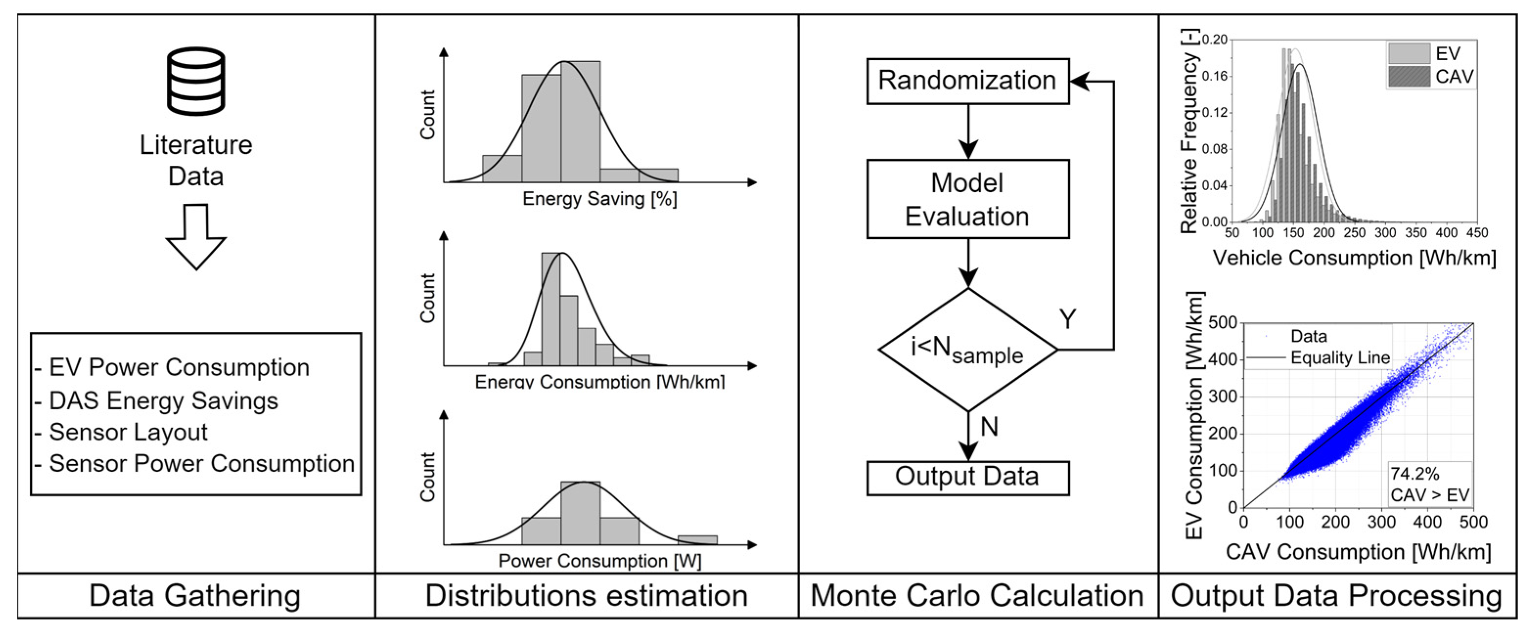
2. Materials and Methods
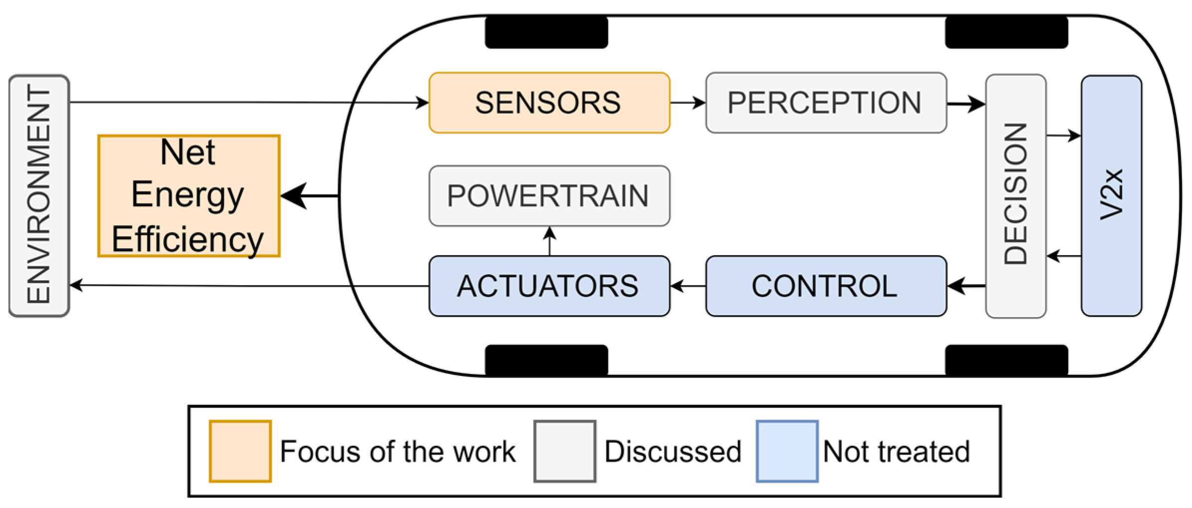
3. CAV Architecture
- (i).
- Observe: the data are gathered from the sensors and, eventually, will be received using infrastructure and other vehicles through V2x connectivity;
- (ii).
- Orient: the data are used to reconstruct the surrounding environment and localise the vehicle;
- (iii).
- Decide: a decision-making algorithm defines the best trajectory to follow to fulfil the mission goal, respecting the constraints;
- (iv).
- Act: the command for the actuators to follow the desired trajectory is generated and injected into the physical layer (i.e., electronic control units and actuators).
Sample Configurations
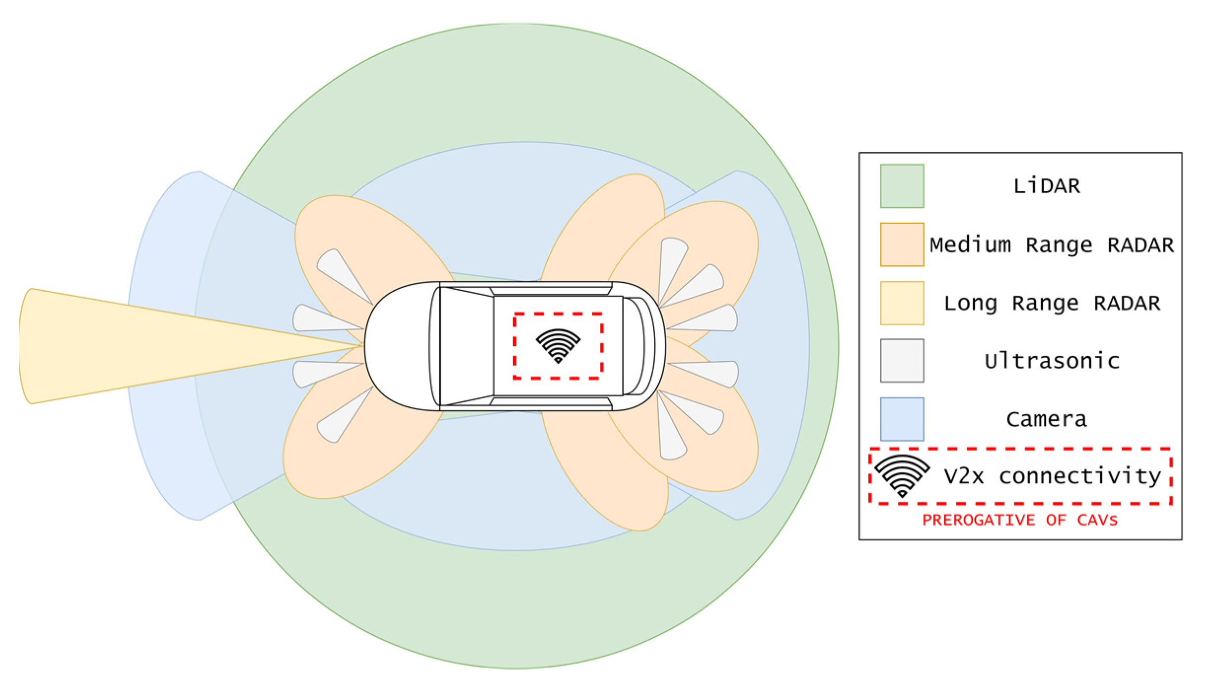
4. Sensors
- On-road vehicle, true world, real scenario testing;
- Sensor testing, true world condition reproduction;
- Sensor testing, tailored simulation test bench, laboratory.
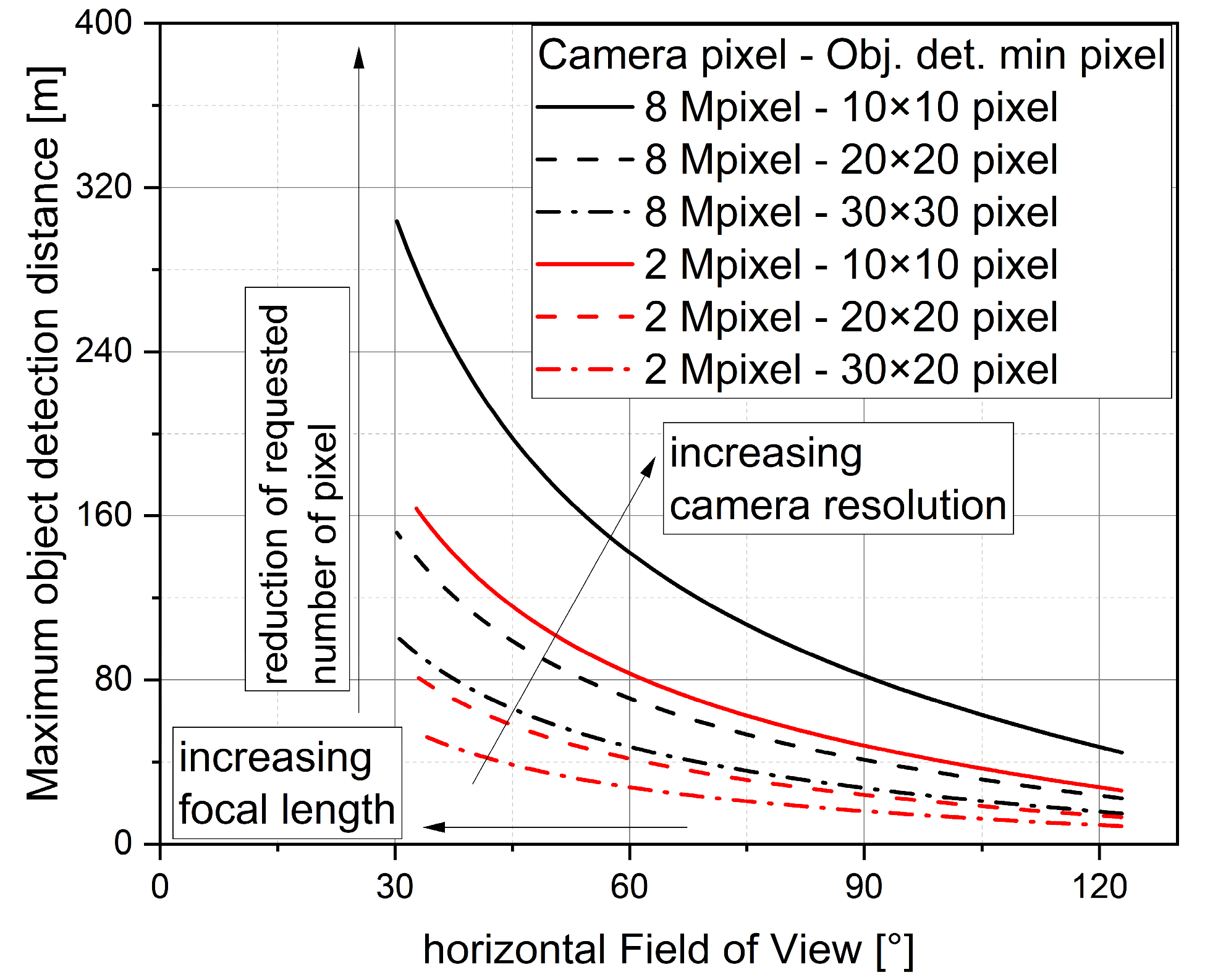
4.1. Camera
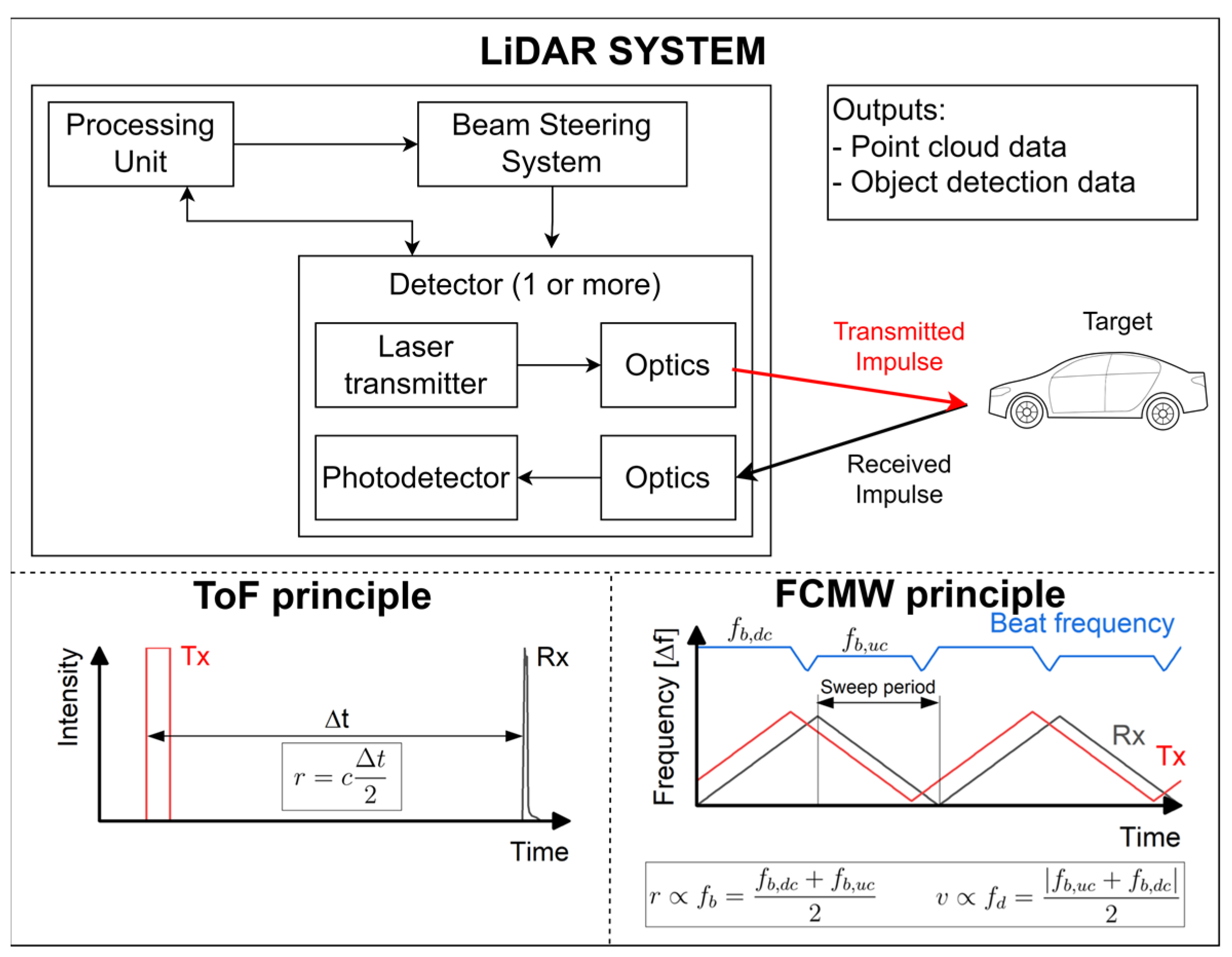
4.2. LiDAR
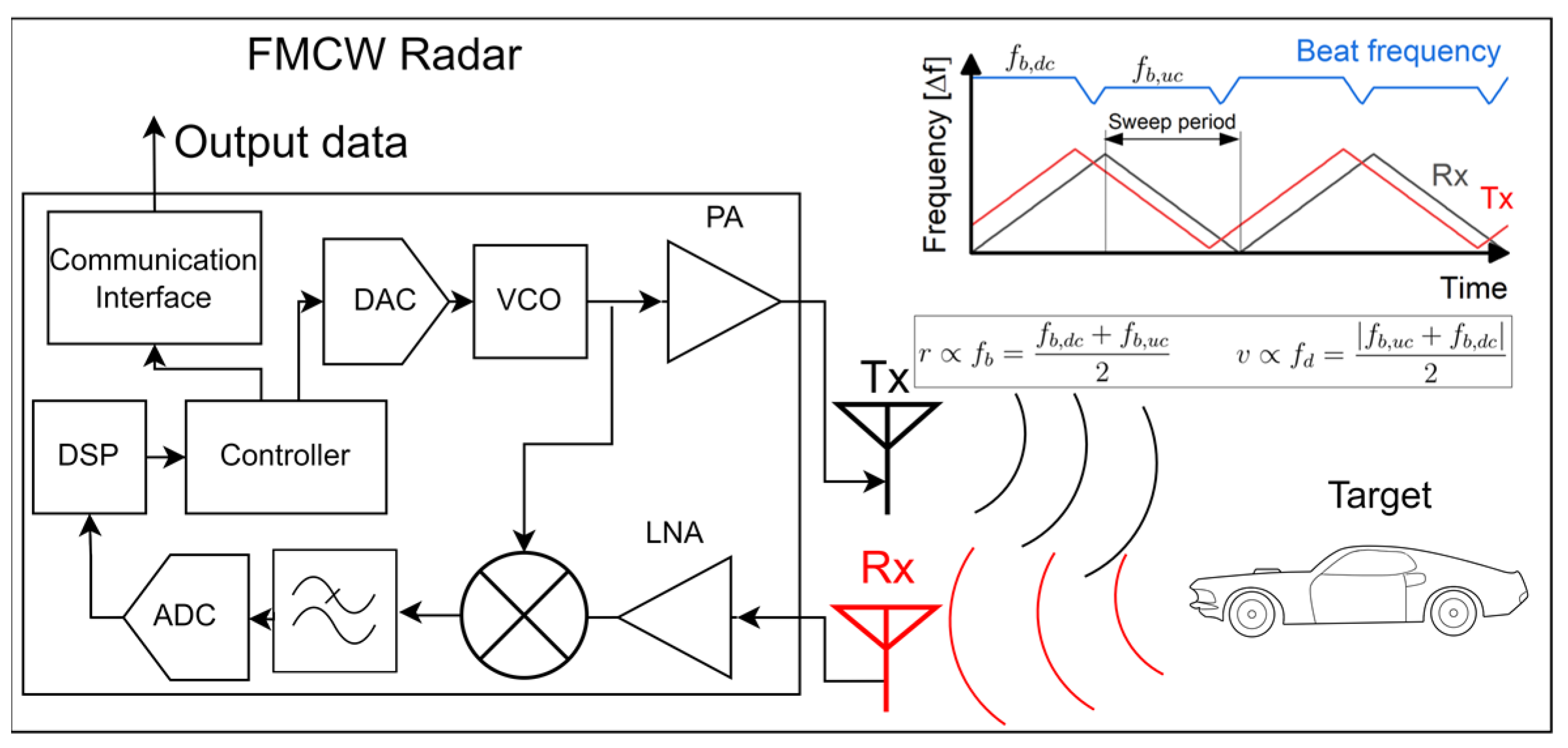
4.3. Radar
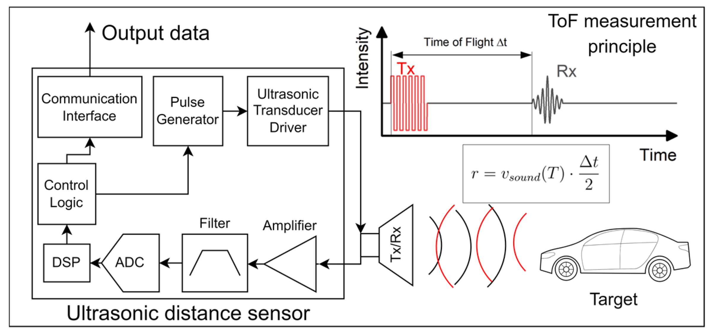
4.4. Ultrasonic
4.5. GNSS
5. An Overview of Data Processing and Management
5.1. Data Generation and Management
5.2. Data Processing
5.3. Data Exploitation for Energy Managament and Efficiency Improvements
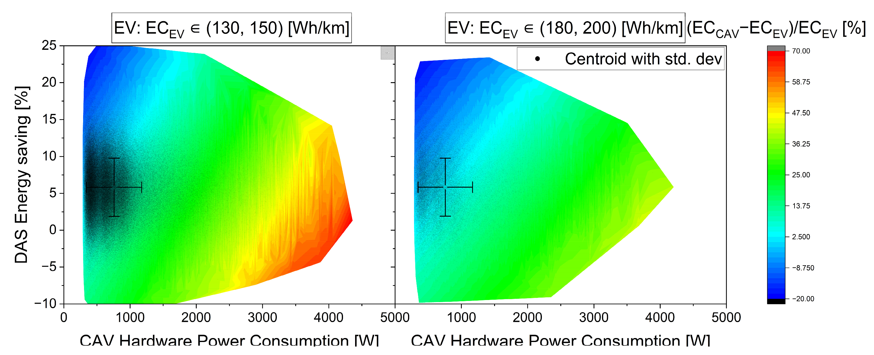
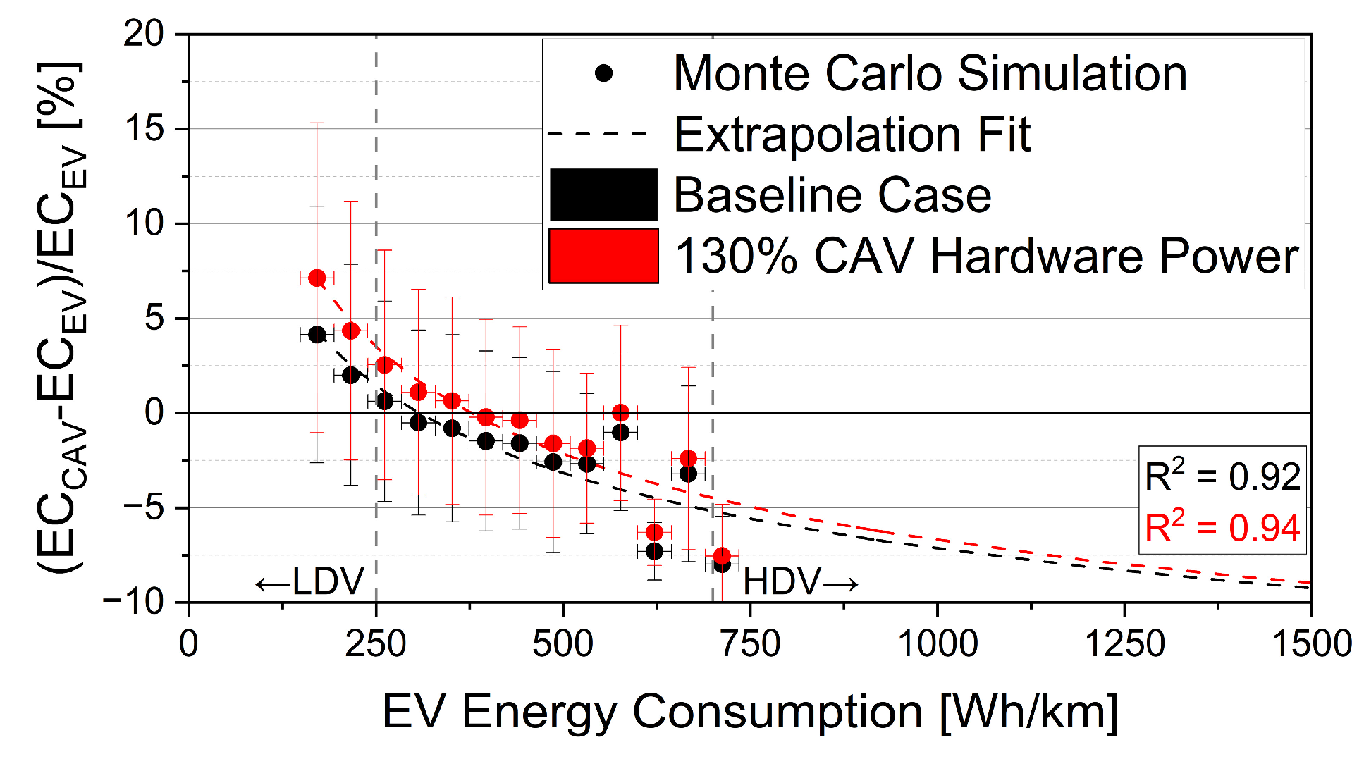
6. Energy Consumption and Impact on Vehicle Usage
7. Conclusions
- CAV architecture likely requires multiple sensors to achieve fully autonomous operation. A proper combination of different sensors can effectively simplify vehicle operations and improve safety and reliability under different and severe operating conditions.
- Regarding sensors, LiDAR can effectively measure and reconstruct the surrounding environment, but its high cost and weather sensitivity limit its application. Automotive radars suffer low angular accuracy but are often used since they can operate in adverse weather. In this scenario, 4D radar has the potential to overcome this limit and aid in reducing the number of required sensors.
- Data management is a crucial point. Sensor data storage and processing should be carefully addressed as they strongly influence vehicle performance. In particular, data elaboration and sensor fusion are key pillars which should be further developed to achieve fully operational CAVs. The improvement of the algorithms should be adequately supported by the production of more powerful and energy-efficient processing units.
- The energy analysis has shown that in an analogy of Maxwell’s demon paradigm, attention should be addressed to the environmental impact of the CAVs. If, as many studies do, the information is considered free, it can be wrongly deduced that the DAS system can effectively reduce the CAV information. However, in reality, the information has a price from both economical and energetical perspectives. In fact, if on one hand, it is possible to leverage data to improve vehicle energy efficiency, on the other hand, producing and elaborating data is energy consuming. Considering both contributions, the hypothetical advantages are not obvious, as the net result is due to their balancing.
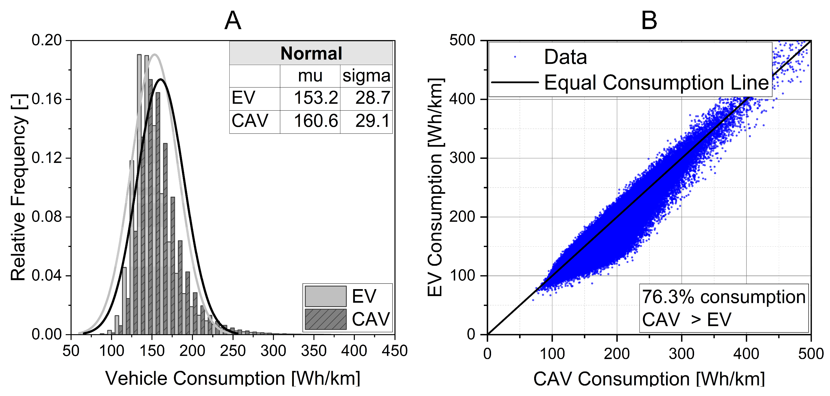
- The Monte Carlo analysis has shown that based on actual data, in about 75% of simulated scenarios, light-duty CAVs consume more energy than EVs. On average, 6% higher energy consumption can be expected by CAVs. Regarding other vehicle classes, the simulation data extrapolation suggests that no or negligible effect could be expected for medium-duty vehicles. Heavy-duty vehicles will probably take advantage of autonomous driving systems due to their higher energy demand, resulting in a lower impact of the DAS system.
Author Contributions
Funding
Data Availability Statement
Acknowledgments
Conflicts of Interest
Abbreviations
| ADAS | Advanced Driving Assistance System |
| AEC | Automotive Electronics Council |
| ASIC | Application Specific Integrated Circuit |
| ASIL | Automotive Safety Integrity Levels |
| AV | Autonomous Vehicle |
| BEV | Battery Electric Vehicle |
| CAN | Controller Area Network |
| CAV | Connected and Autonomous Vehicle |
| CCD | Charge-Coupled Device |
| CMOS | Complementary Metal-Oxide Semiconductor |
| DAS | Driving Automation System |
| DOA | Direction of Arrival |
| DSP | Digital Signal Processor |
| EV | Electric Vehicle |
| FMCW | Frequency Modulated Continuous Wave |
| FoV | Field of View |
| FPGA | Field Programmable Gate Array |
| GMSL | Gigabit Multimedia Serial Link |
| GNSS | Global Navigation Satellite System |
| GPS | Global Positioning System |
| hFoV | Horizontal FoV |
| HPC | High Performance Computing |
| ICT | Information and Communication Technologies |
| IMU | Inertial Measurement Unit |
| LAS | LASer (file format) |
| LiDAR | Light Detection and Ranging |
| LIN | Local Interconnect Network |
| LQR | Linear Quadratic Regulator |
| LRR | Long Range Radar |
| MEMS | Micro Electro-Mechanical Systems |
| MTBF | Mean Time Between Failures |
| MIMO | Multi Input Multi Output |
| MMIC | Monolithic Microwave Integrated Circuit |
| MPC | Model Predictive Control |
| MRR | Medium Range Radar |
| NHTSA | National Highway Traffic Safety Administration |
| OCDMA | Optical Code Division Multiple Access |
| OODA | Observe Orient Decide and Act |
| PCD | Point Cloud Data |
| PID | Proportional-Integral-Derivative |
| RADAR | Radio Detection and Ranging |
| SLAM | Simultaneous Localization and Mapping |
| SONAR | Sound Detection and Ranging |
| SNR | Signal-to-Noise Ratio |
| SRR | Short Range Radar |
| ToF | Time of Flight |
| TOPS | Trillion of Operations per second |
| V2I | Vehicle-to-infrastructure |
| V2V | Vehicle-to-vehicle |
| V2x | Vehicle-to-everything |
| WLTC | Worldwide Harmonised Light Vehicles Test Cycle |
Appendix A

| Manufacturer | Model | Resolution [MP] | Frame Rate [fps] | hFoV × vFOV [°] | Interface | Power Consumption [W] | Note |
|---|---|---|---|---|---|---|---|
| Bosch | Multi-camera system plus | 2 | 30 | 190 × 140 | CAN-FD, Flexray, Ethernet | 30 | |
| Bosch | Multi-purpose camera | 2.6 | 45 | 100 × 48 | |||
| MCNEX | LVDS camera | 1 | 30 | 192 × 120 | LVDS | ||
| MCNEX | 2 | 30 | 114 | ||||
| MCNEX | 3.6 | 30 | 114 | ||||
| Leopard imaging | LI-AR0820- GMSL3-120H | 8.3 | 40 | 140 × 67 | GMSL3 | 1 | |
| Intel | D457 | 1 / 0.93 | 30 / 90 | 90 × 65/87 × 58 | GMSL, USB3 | visual/depth | |
| Intel | D455 | 1 / 0.93 | 30 / 90 | 90 × 65/87 × 58 | USB3 | visual/depth | |
| Luxonis | OAK-D PRO PoE | 12 / 1.0 | 60 / 120 | 95 × 70/127 × 80 | ethernet | 8 | visual/depth |
| Luxonis | OAK-D S2 PoE | 12 / 1.0 | 60 / 120 | 80 × 55/66 × 54 | ethernet | 8 | visual/depth |
| Valeo | Smart Front Camera | 1.7 | 100 × n/a | ||||
| Valeo | Smart Front Camera | 8 | n/a | 120 × n/a | |||
| Valeo | fisheye | 2 | 30 | 195 × 155 | GMSL2, Ethernet | fisheye | |
| TI | TIDA-0500 | 1.3 | 60 | FPD-Link III | 1 | ||
| e-con | NileCAM25_CUXVR | 2 | 65 @ 2Mp/120 @ 1Mp | 105 × 62 | GMSL2 | 11 | |
| FLIR | Ladybug 6 | 72 | 15 @ 72 Mp/30 @ 36 Mp | 360 × 120 | USB3 | 13 | Spherical cam |
| Manufacturer | Model | Year | Technology | Wavelength [nm] | hFOV [deg] | H. Resolution [deg] | vFOV [deg] | V. Resolution [deg] | Frequency [Hz] | Max Range [m] @ Reflectity | Typical Power [W] |
|---|---|---|---|---|---|---|---|---|---|---|---|
| Valeo | SCALA 3° gen | 2023 | 120 | 0.05 | 26 | 0.05 | 190 @ 10% | ||||
| SCALA 2° gen | 2021 | Rot. mirror | 905 | 133 | 0.125/0.25 | 10 | 0.6 | 25 | 200 | 10 | |
| Robosense | RS-LIDAR-M1 | 2021 | Solid state | 905 | 120 | 0.2 | 25 | 0.2 | 10 | 200 | 15 |
| RS-Ruby | 2021 | mechanical | 905 | 360 | 0.2/0.4 | 40 | 0.1 | 10/20 | 200 | 45 | |
| Cepton | Vista®-P60 | 2019 | Solid state | 905 | 60 | 0.25 (10 Hz) 0.27 | 22 | 10 | 200 @ 30% | 10 | |
| Vista®-P90 | Solid state | 905 | 90 | 0.38 | 40 | 0.38 | 10/20 | 200 @ 30% | 10 | ||
| Vista®-X90 | 2020 | Solid state | 90 | 0.13 | 25 | 0.13 | 40 | 200 @ 10% | 12 | ||
| Vista®-x120 | Solid state | 120 | 0.13 | 18/20 | 0.13 | 200 @ 10% | |||||
| Nova | 2021 | 120 | 0.3 | 90 | 0.3 | 30 @ 10% | |||||
| Luminar | Iris | 2022 | 120 | 0.05 | 0–26 | 0.05 | 1–30 | 250 @ 10% | 25 | ||
| Innoviz | InnovizOne | 2016 | 115 | 0.1 | 25 | 0.1 | 5–20 | 250 | |||
| InnovizTwo | 2020 | 120 | 0.05 | 40 | 0.05 | 10–20 | 300 | ||||
| Innoviz360 | 2022 | Rotating | 905 | 360 | 0.05 | 64 | 0.05 | 0.5–25 | 300 | 25 | |
| Ibeo | Next Long range | Solid state | 885 | 11.2 | 0.09 | 5.6 | 0.07 | 25 | 7–10 | ||
| Next Short range | Solid state | 885 | 60 | 0.47 | 30 | 0.38 | 25 | 7–10 | |||
| Next Near range | Solid state | 885 | 120 | 0.94 | 60 | 0.75 | 25 | 7–10 | |||
| LUX 4L | 905 | 110 | 0.25 | 3.2 | 0.8 | 25 | 50 @10% | 7 | |||
| LUX 8L | 905 | 110 | 0.25 | 6.4 | 0.8 | 25 | 50 @10% | 8 | |||
| LUX HD | 905 | 110 | 0.25 | 3.2 | 0.8 | 25 | 30 @10% | 7 | |||
| Innovusion | Jaguar Prime | 2020 | 1550 | 65 | 0.09–0.17/0.19–0.33 | 40 | 0.13 | 6–20 | 300 | 48 | |
| Velodyne | Velarray H800 | 2020 | solid-state | 905 | 120 | 0.26 | 16 | 0.2–0.5 | 10–25 | 200–170 @10% | 13 |
| Baraja | Spectrum HD25 | 2022 | Spectrum-Scan TM | 1550 | 120 | 0.04 | 25 | 0.0125 | 4–30 | 250 @ 10% | 20 |
| Quanergy | M8-Core | 2018 | 905 | 360 | 0.033–0.132 | 20 | 0.033–0.132 | 5–20 | 35 @ 10%/100 @ 80% | 16 | |
| M8-Ultra | 2018 | 905 | 360 | 0.033–0.132 | 20 | 0.033–0.132 | 5–20 | 70 @ 10%/200 @ 80% | 16 | ||
| Continental | SRL121 | 905 | 27 | 11 | 100 | 10 | 1.8 | ||||
| HRL131 | 2022 | 1550 | 128 | 0.05 | 28 | 0.075 | 10 | 300 | |||
| 3D Flash | Flash | 1064 | 120 | 30 | 25 | ||||||
| Sick | Multiscan100 | 850 | 360 | 0.125 | 65 | 1 | 20 | 12 @ 10%/30 @ 90% | 22 | ||
| LMS1000 | 2D | 850 | 275 | 0.75 | 150 | 16@ 10%/36 @ 90% | 18 | ||||
| MRS1000 | 850 | 275 | 0.25 | 7.5 | 1.875 | 50 | 16@ 10%/30 @ 90% | 13 | |||
| LMS511 | 2D | 905 | 190 | 0.1667 | 100 | 26 @ 10% | 22 | ||||
| MRS1000P | 850 | 270 | 0.25 | 7.5 | 12.5/50 | 16@ 10%/30 @ 90% | 13 | ||||
| MRS6000 | 870 | 120 | 0.13 | 15 | 0.625 | 30 @ 10%/75 @ 90% | 20 | ||||
| LRS4000 | 2D | 360 | 25 | 0.02 | 40 @ 10%/130 @ 90% | 13 | |||||
| Microvision | MavinTM | 905 | 0.086 | 0.04 | 30 | 220 | |||||
| Movia | 150 | 0.95 | 81 | 0.76 | 14 | ||||||
| Movia | 60 | 75 | 40 | ||||||||
| Movia | 120 | 37.5 | 60 |
| Manufacturer | Model | Type | Frequency Range [Ghz] | Detect. Range [m] | Range acc. [m] | Update Rate [Hz] | Velocity Precision [m/s] | hFOV [deg] | h. Angle res. [deg] | vFOV [deg] | v. Angle res. [deg] | Power Consumption [W] | Interface |
|---|---|---|---|---|---|---|---|---|---|---|---|---|---|
| Bosch | Front radar | 76–77 | 210 | 0.1 | 0.05 | 120 | 0.1 | 30 | 0.2 | 4 | CAN-FD, Flexray, Ethernet | ||
| Front radar Premium | 76–77 | 302 | 0.1 | 0.04 | 120 | 0.1 | 24 | 0.1 | 15 | CAN-FD, Ethernet | |||
| Corner Radar | 76–77 | 160 | 0.1 | 0.04 | 150 | 0.1 | 30 | 0.2 | 4 | CAN-FD, Flexray, Ethernet | |||
| Continental | SRR600 | Surround | 76–81 | 180 | 20 | 0.03 | 150 | CAN-FD, Ethernet | |||||
| ARS540 | LRR | 76–77 | 300 | ~17 | 120 | 0.1 | 23 | ||||||
| ARS510 | LRR | 76–77 | 210 | ~20 | 100 | 4.8 | |||||||
| ARS441 | LRR | 76–77 | 250 | ~17 | 18 (250 m) 90 (70 m) 150 (20 m) | 8 | |||||||
| SRR520 | SRR | 76–77 | 100 | 20 | 0.02 | 15 | |||||||
| ARS620 | LRR | 76–77 | 280 | 20 | 0.02–0.1 | 60 | CAN-FD, Ethernet | ||||||
| ARS640 | LRR | 76–77 | 300 | ~17 | 60 | 0.1 | 0.1 | 23 | |||||
| APTIV | SSR7 | 4D | 160 | 0.1 | 150 | 6 | 15 | CAN-FD, Ethernet | |||||
| SSR7+ | 4D | 200 | 0.03 | 150 | 3 | 15 | 2 | CAN-FD, Ethernet | |||||
| FLR7 | 4D | 290 | 0.05 | 120 | 2 | 15 | 4 | CAN-FD, Ethernet | |||||
| MRR | 77 | 160 | 33 | 90 | 1 | 5 | |||||||
| ESR | 77 | 174(60) | 20 | 20(90) | |||||||||
| SmartMicro | UMR-97 | 77–81 | 120/55/19 | 0.5/0.3/0.15 | 20 | 0.15 | 100/130/130 | 1 | 15 | 2 | 5 | ||
| UMRR-11 | 76–77 | 175/64 | 0.5/0.25 | 20 | 0.1 | 32/100 | 0.25 | 15 | 0.5 | 6 | |||
| DRVEGRD 152 | 76–77 | 180/66 | 0.45/0.16 | 20 | 0.07 | 10 | 0.25 | 20 | 0.5 | 6 | |||
| DRVEGRD 171 | 76–77 | 240/100/40 | 0.6/0.25/0.1 | 20 | 0.07/0.07/0.14 | 10 | 0.5 | 20 | 0.5 | 7 | |||
| Lintech | CAR30 | SRR | 77–81 | 30 | 0.18 | 20 | 0.25 | 120 | 0.1 | 20 | 2 | CAN |
| Manufacturer | Model | Detection Rage [m] | hFoV × vFOV [°] | Frequency [kHz] | Measurement Rate [Hz] | Power Consumption [W] | Interface |
|---|---|---|---|---|---|---|---|
| Bosch | / | 0.15–5.5 | / | 43–60 | 4/8 | / | / |
| Valeo | / | 0.15–4.1 | 75 × 45 | / | / | 6 | CAN |
| Continental | CUS320 | / | / | / | / | / | / |
| MAGNA | / | 0.1–5.5 | / | / | / | / | / |
| SICK | UC40 | 0.065–6 | / | 400 | 10 | 1.5 | digital |
| UC30 | 0.035–5 | 30 × 30 | 120 | 5 | 1.2 | digital | |
| UM12 | 0.04–0.35 | 30 × 30 | 500 | 30 | 1.2 | analog | |
| UC40 | 0.013–0.25 | 20 × 20 | 380 | 20 | 0.9 | digital | |
| UM18 | 0.12–1.3 | 35 × 35 | 200 | 12 | 1.2 | analog | |
| UM30 | 0.6–8 | 37 × 37 | 80 | 3 | 2.4 | digital | |
| UC12 | 0.02–0.35 | 30 × 30 | 500 | 25 | 1.2 | digital |
References
- Szumska, E.M. Electric Vehicle Charging Infrastructure along Highways in the EU. Energies 2023, 16, 895. [Google Scholar] [CrossRef]
- Pipicelli, M.; Sessa, B.; De Nola, F.; Gimelli, A.; Di Blasio, G. Assessment of Battery–Supercapacitor Topologies of an Electric Vehicle under Real Driving Conditions. Vehicles 2023, 5, 424–445. [Google Scholar] [CrossRef]
- Pipicelli, M.; Sedarsky, D.; Koopmans, L.; Gimelli, A.; Di Blasio, G. Comparative Assessment of Zero CO2 Powertrain for Light Commercial Vehicles; SAE Technical Paper: Warrendale, PA, USA, 2023; p. 2023-24-0150. [Google Scholar] [CrossRef]
- Nastjuk, I.; Herrenkind, B.; Marrone, M.; Brendel, A.B.; Kolbe, L.M. What drives the acceptance of autonomous driving? An investigation of acceptance factors from an end-user’s perspective. Technol. Forecast. Soc. Chang. 2020, 161, 120319. [Google Scholar] [CrossRef]
- Payre, W.; Birrell, S.; Parkes, A.M. Although autonomous cars are not yet manufactured, their acceptance already is. Theor. Issues Ergon. Sci. 2021, 22, 567–580. [Google Scholar] [CrossRef]
- J3016C: Taxonomy and Definitions for Terms Related to Driving Automation Systems for On-Road Motor Vehicles—SAE International. (n.d.). Available online: https://www.sae.org/standards/content/j3016_202104/ (accessed on 28 June 2021).
- Mercedes-Benz Group. Mercedes-Benz—The Front Runner in Automated Driving and Safety Technologies, Mercedes-Benz Group. 2022. Available online: https://group.mercedes-benz.com/innovation/case/autonomous/drive-pilot-2.html (accessed on 6 June 2022).
- Faxér, A.; Jansson, J.; Wilhelmsson, J.; Faleke, M.; Paijkull, M.; Sarasini, S.; Fabricius, V. Shared Shuttle Services S3–Phase 2. 2021. Available online: https://www.drivesweden.net/sites/default/files/2022-10/final-report-for-drive-sweden-projects-s3-092963-2.pdf (accessed on 15 November 2023).
- Nemoto, E.H.; Jaroudi, I.; Fournier, G. Introducing Automated Shuttles in the Public Transport of European Cities: The Case of the AVENUE Project. In Advances in Mobility-as-a-Service Systems; Nathanail, E.G., Adamos, G., Karakikes, I., Eds.; Springer International Publishing: Cham, Switzerland, 2021; pp. 272–285. [Google Scholar] [CrossRef]
- Stange, V.; Kühn, M.; Vollrath, M. Manual drivers’ experience and driving behavior in repeated interactions with automated Level 3 vehicles in mixed traffic on the highway. Transp. Res. Part F Traffic Psychol. Behav. 2022, 87, 426–443. [Google Scholar] [CrossRef]
- Shetty, A.; Yu, M.; Kurzhanskiy, A.; Grembek, O.; Tavafoghi, H.; Varaiya, P. Safety challenges for autonomous vehicles in the absence of connectivity. Transp. Res. Part C Emerg. Technol. 2021, 128, 103133. [Google Scholar] [CrossRef]
- Zhao, L.; Malikopoulos, A.A. Enhanced Mobility With Connectivity and Automation: A Review of Shared Autonomous Vehicle Systems. IEEE Intell. Transp. Syst. Mag. 2022, 14, 87–102. [Google Scholar] [CrossRef]
- Jafarnejad, S.; Codeca, L.; Bronzi, W.; Frank, R.; Engel, T. A Car Hacking Experiment: When Connectivity Meets Vulnerability. In Proceedings of the 2015 IEEE Globecom Workshops (GC Wkshps), San Diego, CA, USA, 6–10 December 2015; pp. 1–6. [Google Scholar] [CrossRef]
- Musa, A.; Pipicelli, M.; Spano, M.; Tufano, F.; De Nola, F.; Di Blasio, G.; Gimelli, A.; Misul, D.A.; Toscano, G. A review of model predictive controls applied to advanced driver-assistance systems. Energies 2021, 14, 7974. [Google Scholar] [CrossRef]
- Papantoniou, P.; Kalliga, V.; Antoniou, C. How autonomous vehicles may affect vehicle emissions on motorways. In Proceedings of the Advances in Mobility-as-a-Service Systems: Proceedings of 5th Conference on Sustainable Urban Mobility, Virtual CSUM2020, Home, Greece, 17–19 June 2020; Springer: Berlin/Heidelberg, Germany, 2021; pp. 296–304. [Google Scholar]
- Pelikan, H.R.M. Why Autonomous Driving Is So Hard: The Social Dimension of Traffic. In Proceedings of the Companion of the 2021 ACM/IEEE International Conference on Human-Robot Interaction, Association for Computing Machinery, New York, NY, USA, 8–11 March 2021; pp. 81–85. [Google Scholar] [CrossRef]
- Khan, M.A.; El Sayed, H.; Malik, S.; Zia, M.T.; Alkaabi, N.; Khan, J. A journey towards fully autonomous driving—Fueled by a smart communication system. Veh. Commun. 2022, 36, 100476. [Google Scholar] [CrossRef]
- Kroese, D.P.; Brereton, T.; Taimre, T.; Botev, Z.I. Why the Monte Carlo method is so important today. WIREs Comput. Stat. 2014, 6, 386–392. [Google Scholar] [CrossRef]
- Torkjazi, M.; Raz, A.K. Taxonomy for System of Autonomous Systems. In Proceedings of the 2022 17th Annual System of Systems Engineering Conference (SOSE), Rochester, NY, USA, 7–11 June 2022; pp. 198–203. [Google Scholar] [CrossRef]
- Mallozzi, P.; Pelliccione, P.; Knauss, A.; Berger, C.; Mohammadiha, N. Autonomous Vehicles: State of the Art, Future Trends, and Challenges. In Automotive Systems and Software Engineering: State of the Art and Future Trends; Dajsuren, Y., van den Brand, M., Eds.; Springer International Publishing: Cham, Switzerland, 2019; pp. 347–367. [Google Scholar] [CrossRef]
- Azam, S.; Munir, F.; Sheri, A.M.; Kim, J.; Jeon, M. System, Design and Experimental Validation of Autonomous Vehicle in an Unconstrained Environment. Sensors 2020, 20, 5999. [Google Scholar] [CrossRef] [PubMed]
- Gonzalez, D.; Perez, J.; Milanes, V.; Nashashibi, F. A Review of Motion Planning Techniques for Automated Vehicles. IEEE Trans. Intell. Transp. Syst. 2016, 17, 1135–1145. [Google Scholar] [CrossRef]
- Lee, S.; Jung, Y.; Park, Y.-H.; Kim, S.-W. Design of V2X-based vehicular contents centric networks for autonomous driving. IEEE Trans. Intell. Transp. Syst. 2021, 23, 13526–13537. [Google Scholar] [CrossRef]
- Marin-Plaza, P.; Hussein, A.; Martin, D.; de la Escalera, A. Global and Local Path Planning Study in a ROS-Based Research Platform for Autonomous Vehicles. J. Adv. Transp. 2018, 2018, e6392697. [Google Scholar] [CrossRef]
- Song, X.; Gao, H.; Ding, T.; Gu, Y.; Liu, J.; Tian, K. A Review of the Motion Planning and Control Methods for Automated Vehicles. Sensors 2023, 23, 6140. [Google Scholar] [CrossRef]
- Warren, M.E. Automotive LIDAR Technology. In 2019 Symposium on VLSI Circuits; IEEE: New York, NY, USA, 2019; pp. C254–C255. [Google Scholar] [CrossRef]
- True Redundancy, Mobileye. (n.d.). Available online: https://www.mobileye.com/technology/true-redundancy/ (accessed on 22 September 2023).
- Reschka, A. Safety Concept for Autonomous Vehicles. In MAutonomous Driving: Technical, Legal and Social Aspects; Maurer, M., Gerdes, J.C., Lenz, B., Winner, H., Eds.; Springer: Berlin/Heidelberg, Germany, 2016; pp. 473–496. [Google Scholar] [CrossRef]
- Yan, Z.; Sun, L.; Krajnik, T.; Ruichek, Y. EU Long-term Dataset with Multiple Sensors for Autonomous Driving. In Proceedings of the 2020 IEEE/RSJ International Conference on Intelligent Robots and Systems (IROS), Las Vegas, NV, USA, 24 October 2020–24 January 2021; pp. 10697–10704. [Google Scholar] [CrossRef]
- Everything You Need to Know about Autonom® Shuttle Evo, NAVYA. (n.d.). Available online: https://www.navya.tech/en/everything-you-need-to-know-about-autonom-shuttle-evo/ (accessed on 21 September 2023).
- Mobileye DriveTM|Self-Driving System for Autonomous MaaS, Mobileye. (n.d.). Available online: https://www.mobileye.com/newsletter-sign-up/ (accessed on 22 September 2023).
- Mobileye SuperVisionTM for Hands-Free ADAS, Mobileye. (n.d.). Available online: https://www.mobileye.com/super-vision/ (accessed on 4 June 2022).
- Hardware NVIDIA Drive per Auto a Guida Autonoma, NVIDIA. (n.d.). Available online: https://www.nvidia.com/it-it/self-driving-cars/drive-platform/hardware/ (accessed on 27 September 2023).
- Mobileye Self-Driving Mobility Services, Mobileye. (n.d.). Available online: https://www.mobileye.com/mobility-as-a-service/ (accessed on 4 June 2022).
- van Dijk, L.; Sporer, G. Functional safety for automotive ethernet networks. J. Traffic Transp. Eng. 2018, 6, 176–182. [Google Scholar] [CrossRef]
- Sheeny, M.; De Pellegrin, E.; Mukherjee, S.; Ahrabian, A.; Wang, S.; Wallace, A. RADIATE: A Radar Dataset for Automotive Perception in Bad Weather. In Proceedings of the 2021 IEEE International Conference on Robotics and Automation (ICRA), Xi’an, China, 30 May–5 June 2021; pp. 1–7. [Google Scholar] [CrossRef]
- Rasshofer, R.H.; Spies, M.; Spies, H. Influences of weather phenomena on automotive laser radar systems. Adv. Radio Sci. 2011, 9, 49–60. [Google Scholar] [CrossRef]
- Espineira, J.P.; Robinson, J.; Groenewald, J.; Chan, P.H.; Donzella, V. Realistic LiDAR With Noise Model for Real-Time Testing of Automated Vehicles in a Virtual Environment. IEEE Sensors J. 2021, 21, 9919–9926. [Google Scholar] [CrossRef]
- Zhao, J.; Li, Y.; Zhu, B.; Deng, W.; Sun, B. Method and Applications of Lidar Modeling for Virtual Testing of Intelligent Vehicles. IEEE Trans. Intell. Transp. Syst. 2021, 22, 2990–3000. [Google Scholar] [CrossRef]
- Reway, F.; Huber, W.; Ribeiro, E.P. Test Methodology for Vision-Based ADAS Algorithms with an Automotive Camera-in-the-Loop. In Proceedings of the 2018 IEEE International Conference on Vehicular Electronics and Safety (ICVES), Madrid, Spain, 12–14 September 2018; pp. 1–7. [Google Scholar] [CrossRef]
- Jegham, I.; Ben Khalifa, A. Pedestrian detection in poor weather conditions using moving camera. In Proceedings of the 2017 IEEE/ACS 14th International Conference on Computer Systems and Applications (AICCSA), Hammamet, Tunisia, 30 October 2017–3 November 2017; pp. 358–362. [Google Scholar] [CrossRef]
- Anwar, I.; Khosla, A. Vision enhancement through single image fog removal. Eng. Sci. Technol. Int. J. 2017, 20, 1075–1083. [Google Scholar] [CrossRef]
- Meng, X.; Liu, Y.; Fan, L.; Fan, J. YOLOv5s-Fog: An Improved Model Based on YOLOv5s for Object Detection in Foggy Weather Scenarios. Sensors 2023, 23, 5321. [Google Scholar] [CrossRef] [PubMed]
- Bijelic, M.; Gruber, T.; Ritter, W. A Benchmark for Lidar Sensors in Fog: Is Detection Breaking Down? In Proceedings of the 2018 IEEE Intelligent Vehicles Sympo-sium (IV), Changshu, China, 26–30 June 2018; pp. 760–767. [Google Scholar] [CrossRef]
- Kutila, M.; Pyykönen, P.; Holzhüter, H.; Colomb, M.; Duthon, P. Automotive LiDAR performance verification in fog and rain. In Proceedings of the 2018 21st International Conference on Intelligent Transportation Systems (ITSC), Maui, HI, USA, 4–7 November 2018; pp. 1695–1701. [Google Scholar] [CrossRef]
- Sindagi, V.A.; Zhou, Y.; Tuzel, O. MVX-Net: Multimodal VoxelNet for 3D Object Detection. In Proceedings of the 2019 International Conference on Robotics and Automation (ICRA), Montreal, QC, Canada, 20–24 May 2019; pp. 7276–7282. [Google Scholar] [CrossRef]
- Arage, A.; Steffens, W.M.; Kuehnle, G.; Jakoby, R. Effects of water and ice layer on automotive radar. In Proceedings of the German Microwave Conference, Citeseer, Taiwan, China, 8–11 October 2006. [Google Scholar]
- Vargas, J.; Alsweiss, S.; Toker, O.; Razdan, R.; Santos, J. An Overview of Autonomous Vehicles Sensors and Their Vulnerability to Weather Conditions. Sensors 2021, 21, 5397. [Google Scholar] [CrossRef] [PubMed]
- Herpel, T.; Lauer, C.; German, R.; Salzberger, J. Trade-off between coverage and robustness of automotive environment sensor systems. In Proceedings of the 2008 International Conference on Intelligent Sensors, Sensor Networks and Information Processing, Sydney, NSW, Australia, 15–18 December 2008; pp. 551–556. [Google Scholar] [CrossRef]
- Liu, Z.; Jiang, H.; Tan, H.; Zhao, F. An Overview of the Latest Progress and Core Challenge of Autonomous Vehicle Technologies. MATEC Web Conf. 2020, 308, 06002. [Google Scholar] [CrossRef][Green Version]
- Do, T.H.; Yoo, M. Visible light communication based vehicle positioning using LED street light and rolling shutter CMOS sensors. Opt. Commun. 2018, 407, 112–126. [Google Scholar] [CrossRef]
- Horaud, R.; Hansard, M.; Evangelidis, G.; Ménier, C. An overview of depth cameras and range scanners based on time-of-flight technologies. Mach. Vis. Appl. 2016, 27, 1005–1020. [Google Scholar] [CrossRef]
- Endres, F.; Hess, J.; Sturm, J.; Cremers, D.; Burgard, W. 3-D Mapping With an RGB-D Camera. IEEE Trans. Robot. 2014, 30, 177–187. [Google Scholar] [CrossRef]
- Sivaraman, S.; Trivedi, M.M. Looking at Vehicles on the Road: A Survey of Vision-Based Vehicle Detection, Tracking, and Behavior Analysis. IEEE Trans. Intell. Transp. Syst. 2013, 14, 1773–1795. [Google Scholar] [CrossRef]
- Stallkamp, J.; Schlipsing, M.; Salmen, J.; Igel, C. Man vs. computer: Benchmarking machine learning algorithms for traffic sign recognition. Neural Netw. 2012, 32, 323–332. [Google Scholar] [CrossRef]
- Ciberlin, J.; Grbic, R.; Teslić, N.; Pilipović, M. Object detection and object tracking in front of the vehicle using front view camera. In Proceedings of the 2019 Zooming Innovation in Consumer Technologies Conference (ZINC), Novi Sad, Serbia, 29–30 May 2019; pp. 27–32. [Google Scholar] [CrossRef]
- Drulea, M.; Szakats, I.; Vatavu, A.; Nedevschi, S. Omnidirectional stereo vision using fisheye lenses. In Proceedings of the 2014 IEEE 10th International Conference on Intelligent Computer Communication and Processing (ICCP), Cluj-Napoca, Cluj, Romania, 4–6 September 2014; pp. 251–258. [Google Scholar] [CrossRef]
- Florea, H.; Petrovai, A.; Giosan, I.; Oniga, F.; Varga, R.; Nedevschi, S. Enhanced Perception for Autonomous Driving Using Semantic and Geometric Data Fusion. Sensors 2022, 22, 5061. [Google Scholar] [CrossRef]
- Ignatious, H.A.; Sayed, H.-E.; Khan, M. An overview of sensors in Autonomous Vehicles. Procedia Comput. Sci. 2022, 198, 736–741. [Google Scholar] [CrossRef]
- Li, Y.; Ibanez-Guzman, J. Lidar for Autonomous Driving: The Principles, Challenges, and Trends for Automotive Lidar and Perception Systems. IEEE Signal Process. Mag. 2020, 37, 50–61. [Google Scholar] [CrossRef]
- Raj, T.; Hashim, F.H.; Huddin, A.B.; Ibrahim, M.F.; Hussain, A. A Survey on LiDAR Scanning Mechanisms. Electronics 2020, 9, 741. [Google Scholar] [CrossRef]
- Zhang, F.; Yi, L.; Qu, X. Simultaneous measurements of velocity and distance via a dual-path FMCW lidar system. Opt. Commun. 2020, 474, 126066. [Google Scholar] [CrossRef]
- Muckenhuber, S.; Holzer, H.; Bockaj, Z. Automotive Lidar Modelling Approach Based on Material Properties and Lidar Capabilities. Sensors 2020, 20, 3309. [Google Scholar] [CrossRef]
- Kim, G.; Eom, J.; Park, Y. Investigation on the occurrence of mutual interference between pulsed terrestrial LIDAR scanners. In Proceedings of the 2015 IEEE Intelligent Vehicles Symposium (IV), Seoul, Korea, 28 June–1 July 2015; pp. 437–442. [Google Scholar] [CrossRef]
- Hwang, I.-P.; Yun, S.-J.; Lee, C.-H. Study on the Frequency-Modulated Continuous-Wave LiDAR Mutual Interference. In Proceedings of the 2019 IEEE 19th Interna-tional Conference on Communication Technology (ICCT), Xi’an, China, 16–19 October 2019; pp. 1053–1056. [Google Scholar] [CrossRef]
- Fersch, T.; Weigel, R.; Koelpin, A. A CDMA Modulation Technique for Automotive Time-of-Flight LiDAR Systems. IEEE Sensors J. 2017, 17, 3507–3516. [Google Scholar] [CrossRef]
- Hwang, I.-P.; Lee, C.-H. Mutual Interferences of a True-Random LiDAR With Other LiDAR Signals. IEEE Access 2020, 8, 124123–124133. [Google Scholar] [CrossRef]
- Yin, W.; He, W.; Gu, G.; Chen, Q. Approach for LIDAR signals with multiple returns. Appl. Opt. 2014, 53, 6963–6969. [Google Scholar] [CrossRef]
- Asmann, A.; Stewart, B.; Wallace, A.M. Deep Learning for LiDAR Waveforms with Multiple Returns. In Proceedings of the 2020 28th European Signal Processing Conference (EUSIPCO), Amsterdam, The Netherlands, 18–21 January 2021; pp. 1571–1575. [Google Scholar] [CrossRef]
- Heinzler, R.; Schindler, P.; Seekircher, J.; Ritter, W.; Stork, W. Weather Influence and Classification with Automotive Lidar Sensors. In Proceedings of the 2019 IEEE Intelligent Vehicles Sympo-sium (IV), Paris, France, 9–12 June 2019; pp. 1527–1534. [Google Scholar] [CrossRef]
- Hecht, J. Lidar for Self-Driving Cars. Opt. Photon- News 2018, 29, 26–33. [Google Scholar] [CrossRef]
- Velodyne’s Guide to Lidar Wavelengths, Velodyne Lidar. 2018. Available online: https://velodynelidar.com/blog/guide-to-lidar-wavelengths/ (accessed on 7 June 2022).
- McManamon, P.F.; Banks, P.S.; Beck, J.D.; Fried, D.G.; Huntington, A.S.; Watson, E.A. Comparison of flash lidar detector options. Opt. Eng. 2017, 56, 031223. [Google Scholar] [CrossRef]
- Li, N.; Ho, C.P.; Xue, J.; Lim, L.W.; Chen, G.; Fu, Y.H.; Lee, L.Y.T. A Progress Review on Solid-State LiDAR and Nanophotonics-Based LiDAR Sensors. Laser Photon- Rev. 2022, 16. [Google Scholar] [CrossRef]
- S3 Series, Quanergy. (n.d.). Available online: https://quanergy.com/products/s3/ (accessed on 14 June 2022).
- Waldschmidt, C.; Hasch, J.; Menzel, W. Automotive Radar—From First Efforts to Future Systems. IEEE J. Microw. 2021, 1, 135–148. [Google Scholar] [CrossRef]
- Norouzian, F.; Hoare, E.G.; Marchetti, E.; Cherniakov, M.; Gashinova, M. Next Generation, Low-THz Automotive Radar—The potential for frequencies above 100 GHz. In Proceedings of the 2019 20th In-ternational Radar Symposium (IRS), Ulm, Germany, 26–28 June 2019; pp. 1–7. [Google Scholar] [CrossRef]
- Martinez-Vazquez, M. Overview of design challenges for automotive radar MMICs. In Proceedings of the 2021 IEEE International Electron Devices Meeting (IEDM), San Francisco, CA, USA, 11–16 December 2021; pp. 4.1.1–4.1.3. [Google Scholar] [CrossRef]
- Yamano, S.; Higashida, H.; Shono, M.; Matsui, S.; Tamaki, T.; Yagi, H.; Asanuma, H. 76GHz millimeter wave automobile radar using single chip MMIC. Fujitsu Ten Technol. J. 2004, 23, 12–19. [Google Scholar]
- Ritter, P. Toward a fully integrated automotive radar system-on-chip in 22 nm FD-SOI CMOS. Int. J. Microw. Wirel. Technol. 2021, 13, 523–531. [Google Scholar] [CrossRef]
- Zhang, A.; Nowruzi, F.E.; Laganiere, R. RADDet: Range-Azimuth-Doppler based Radar Object Detection for Dynamic Road Users. In Proceedings of the IEEE Computer Society, Burnaby, BC, Canada, 26–28 May 2021; pp. 95–102. [Google Scholar] [CrossRef]
- Tong, Z.T.Z.; Reuter, R.; Fujimoto, M. Fast chirp FMCW radar in automotive applications. In Proceedings of the IET International Radar Conference 2015, Washington, DC, USA, 11–15 May 2015; pp. 1–4. [Google Scholar] [CrossRef]
- Bilik, I.; Bialer, O.; Villeval, S.; Sharifi, H.; Kona, K.; Pan, M.; Persechini, D.; Musni, M.; Geary, K. Geary, Automotive MIMO radar for urban environments. In Proceedings of the 2016 IEEE Radar Conference (RadarConf), Philadelphia, PA, USA, 2–6 May 2016; pp. 1–6. [Google Scholar] [CrossRef]
- Sit, Y.L.; Nguyen, T.T.; Sturm, C.; Zwick, T. 2D radar imaging with velocity estimation using a MIMO OFDM-based radar for automotive applications. In Proceedings of the 2013 European Radar Conference, Nuremberg, Germany, 5 October 2013; pp. 145–148. Available online: https://ieeexplore.ieee.org/abstract/document/6689134 (accessed on 19 October 2023).
- Vasanelli, C.; Batra, R.; Waldschmidt, C. Optimization of a MIMO radar antenna system for automotive applications. In Proceedings of the 2017 11th European Conference on Antennas and Propagation (EUCAP), Paris, France, 19–24 March 2017; pp. 1113–1117. [Google Scholar] [CrossRef]
- Stolz, M.; Wolf, M.; Meinl, F.; Kunert, M.; Menzel, W. A New Antenna Array and Signal Processing Concept for an Automotive 4D Radar. In Proceedings of the 2018 15th European Ra-dar Conference (EuRAD), Madrid, Spain, 26–28 September 2018; pp. 63–66. [Google Scholar] [CrossRef]
- Sun, S.; Zhang, Y.D. 4D Automotive Radar Sensing for Autonomous Vehicles: A Sparsity-Oriented Approach. IEEE J. Sel. Top. Signal Process. 2021, 15, 879–891. [Google Scholar] [CrossRef]
- Hakobyan, G.; Yang, B. High-Performance Automotive Radar: A Review of Signal Processing Algorithms and Modulation Schemes. IEEE Signal Process. Mag. 2019, 36, 32–44. [Google Scholar] [CrossRef]
- Hosur, P.; Shettar, R.B.; Potdar, M. Environmental awareness around vehicle using ultrasonic sensors. In Proceedings of the 2016 International Conference on Ad-vances in Computing, Communications and Informatics (ICACCI), Jaipur, India, 21–24 September 2016; pp. 1154–1159. [Google Scholar] [CrossRef]
- Rasshofer, R.H.; Gresser, K. Automotive Radar and Lidar Systems for Next Generation Driver Assistance Functions. Adv. Radio Sci. 2005, 3, 205–209. [Google Scholar] [CrossRef]
- Balasubramanian, A.B.; Sastry, K.V.; Magee, D.P.; Taylor, D.G. Transmitter and Receiver Enhancements for Ultrasonic Distance Sensing Systems. IEEE Sensors J. 2022, 22, 10692–10698. [Google Scholar] [CrossRef]
- Khan, J. Using ADAS sensors in implementation of novel automotive features for increased safety and guidance. In Proceedings of the 2016 3rd International Conference on Signal Processing and Integrated Networks (SPIN), Noida, India, 11–12 February 2016; IEEE: New York, NY, USA, 2016; pp. 753–758. [Google Scholar] [CrossRef]
- Tong, F.; Tso, S.; Xu, T. A high precision ultrasonic docking system used for automatic guided vehicle. Sensors Actuators A Phys. 2005, 118, 183–189. [Google Scholar] [CrossRef]
- Canali, C.; De Cicco, G.; Morten, B.; Prudenziati, M.; Taroni, A. A Temperature Compensated Ultrasonic Sensor Operating in Air for Distance and Proximity Measurements. IEEE Trans. Ind. Electron. 1982, IE-29, 336–341. [Google Scholar] [CrossRef]
- Xu, W.; Yan, C.; Jia, W.; Ji, X.; Liu, J. Analyzing and Enhancing the Security of Ultrasonic Sensors for Autonomous Vehicles. IEEE Internet Things J. 2018, 5, 5015–5029. [Google Scholar] [CrossRef]
- Toa, M.; Whitehead, A. Ultrasonic Sensing Basics; Texas Instruments: Dallas, TX, USA, 2020; pp. 53–75. [Google Scholar]
- Li, S.E.; Li, G.; Yu, J.; Liu, C.; Cheng, B.; Wang, J.; Li, K. Kalman filter-based tracking of moving objects using linear ultrasonic sensor array for road vehicles. Mech. Syst. Signal Process. 2018, 98, 173–189. [Google Scholar] [CrossRef]
- Imou, K.; Kaizu, Y.; Yokoyama, S.; Nakamura, T. Ultrasonic Doppler Speed Sensor for Agricultural Vehicles: Effects of Pitch Angle and Measurements of Velocity Vector Components. Agric. Eng. Int. CIGR J. 2008. Available online: https://cigrjournal.org/index.php/Ejounral/article/view/1232 (accessed on 24 September 2023).
- Gluck, T.; Kravchik, M.; Chocron, S.; Elovici, Y.; Shabtai, A. Spoofing Attack on Ultrasonic Distance Sensors Using a Continuous Signal. Sensors 2020, 20, 6157. [Google Scholar] [CrossRef]
- Lou, J.; Yan, Q.; Hui, Q.; Zeng, H. SoundFence: Securing Ultrasonic Sensors in Vehicles Using Physical-Layer Defense. In Proceedings of the 2021 18th Annual IEEE International Conference on Sensing, Communication, and Networking (SECON), Rome, Italy, 6–9 July 2021; pp. 1–9. [Google Scholar] [CrossRef]
- Joubert, N.; Reid, T.G.R.; Noble, F. Developments in Modern GNSS and Its Impact on Autonomous Vehicle Architectures. In Proceedings of the 2020 IEEE Intelligent Vehicles Symposium (IV), Las Vegas, NV, USA, 19 October–13 November 2020; pp. 2029–2036. [Google Scholar] [CrossRef]
- Bolla, P.; Borre, K. Performance analysis of dual-frequency receiver using combinations of GPS L1, L5, and L2 civil signals. J. Geodesy 2019, 93, 437–447. [Google Scholar] [CrossRef]
- Zhi, Z.; Liu, D.; Liu, L. A performance compensation method for GPS/INS integrated navigation system based on CNN–LSTM during GPS outages. Measurement 2022, 188, 110516. [Google Scholar] [CrossRef]
- Xiong, L.; Xia, X.; Lu, Y.; Liu, W.; Gao, L.; Song, S.; Yu, Z. IMU-Based Automated Vehicle Body Sideslip Angle and Attitude Estimation Aided by GNSS Using Parallel Adaptive Kalman Filters. IEEE Trans. Veh. Technol. 2020, 69, 10668–10680. [Google Scholar] [CrossRef]
- Liu, W.; Li, Z.; Sun, S.; Gupta, M.K.; Du, H.; Malekian, R.; Sotelo, M.A.; Li, W. Design a Novel Target to Improve Positioning Accuracy of Autonomous Vehicular Navigation System in GPS Denied Environments. IEEE Trans. Ind. Informatics 2021, 17, 7575–7588. [Google Scholar] [CrossRef]
- Chen, L.; Zheng, F.; Gong, X.; Jiang, X. GNSS High-Precision Augmentation for Autonomous Vehicles: Requirements, Solution, and Technical Challenges. Remote. Sens. 2023, 15, 1623. [Google Scholar] [CrossRef]
- Ma, Y.; Wang, Z.; Yang, H.; Yang, L. Artificial intelligence applications in the development of autonomous vehicles: A survey. Ieee/caa J. Autom. Sin. 2020, 7, 315–329. [Google Scholar] [CrossRef]
- Pillmann, J.; Wietfeld, C.; Zarcula, A.; Raugust, T.; Alonso, D.C. Novel common vehicle information model (CVIM) for future automotive vehicle big data marketplaces. In Proceedings of the 2017 IEEE Intelligent Vehicles Symposium (IV), Los Angeles, CA, USA, 11–14 June 2017; pp. 1910–1915. [Google Scholar] [CrossRef]
- Chen, Q. Airborne lidar data processing and information extraction. Photogramm. Eng. Remote Sens. 2007, 73, 109. [Google Scholar]
- Isenburg, M. LASzip: Lossless compression of LiDAR data. Photogramm. Eng. Remote Sens. 2013, 79, 209–217. [Google Scholar] [CrossRef]
- Béjar-Martos, J.A.; Rueda-Ruiz, A.J.; Ogayar-Anguita, C.J.; Segura-Sánchez, R.J.; López-Ruiz, A. Strategies for the Storage of Large LiDAR Datasets—A Performance Comparison. Remote. Sens. 2022, 14, 2623. [Google Scholar] [CrossRef]
- Biasizzo, A.; Novak, F. Hardware Accelerated Compression of LIDAR Data Using FPGA Devices. Sensors 2013, 13, 6405–6422. [Google Scholar] [CrossRef] [PubMed]
- Zinner, H. Automotive Ethernet and SerDes in Competition. ATZelectronics Worldw. 2020, 15, 40–43. [Google Scholar] [CrossRef]
- Zaarane, I.A.; Slimani, W.; Al Okaishi, I.; Atouf, A. Hamdoun, Distance measurement system for autonomous vehicles using stereo camera. Array 2020, 5, 100016. [Google Scholar] [CrossRef]
- Masoumian, A.; Rashwan, H.A.; Cristiano, J.; Asif, M.S.; Puig, D. Monocular Depth Estimation Using Deep Learning: A Review. Sensors 2022, 22, 5353. [Google Scholar] [CrossRef] [PubMed]
- Wu, W.; Zhang, L.; Wang, Y. A PVT-Robust Analog Baseband With DC Offset Cancellation for FMCW Automotive Radar. IEEE Access 2019, 7, 43249–43257. [Google Scholar] [CrossRef]
- He, H.; Li, Y.; Tan, J. Rotational Coordinate Transformation for Visual-Inertial Sensor Fusion. In Social Robotics; Agah, A., Cabibihan, J.-J., Howard, A.M., Salichs, M.A., He, H., Eds.; Springer International Publishing: Cham, Switzerland, 2016; pp. 431–440. [Google Scholar]
- Cao, J.; Song, C.; Song, S.; Xiao, F.; Peng, S. Lane Detection Algorithm for Intelligent Vehicles in Complex Road Conditions and Dynamic Environments. Sensors 2019, 19, 3166. [Google Scholar] [CrossRef]
- Saxena, A.; Prasad, M.; Gupta, A.; Bharill, N.; Patel, O.P.; Tiwari, A.; Er, M.J.; Ding, W.; Lin, C.-T. A review of clustering techniques and developments. Neurocomputing 2017, 267, 664–681. [Google Scholar] [CrossRef]
- Beltran, J.; Guindel, C.; Moreno, F.M.; Cruzado, D.; Garcia, F.; De La Escalera, A. BirdNet: A 3D Object Detection Framework from LiDAR Information. In Proceedings of the 2018 21st International Conference on Intelligent Transportation Systems (ITSC), Maui, HI, USA, 4–7 November 2018; pp. 3517–3523. [Google Scholar] [CrossRef]
- Cao, X.; Lan, J.; Li, X.R.; Liu, Y. Extended Object Tracking Using Automotive Radar. In Proceedings of the 2018 21st International Conference on Information Fu-sion (FUSION), Cambridge, UK, 10–13 July 2018; pp. 1–5. [Google Scholar] [CrossRef]
- Masmoudi, M.; Ghazzai, H.; Frikha, M.; Massoud, Y. Object Detection Learning Techniques for Autonomous Vehicle Applications. In Proceedings of the 2019 IEEE International Conference on Vehicular Electronics and Safety (ICVES), Cairo, Egypt, 4–6 September 2019; pp. 1–5. [Google Scholar] [CrossRef]
- Jahromi, B.S.; Tulabandhula, T.; Cetin, S. Real-Time Hybrid Multi-Sensor Fusion Framework for Perception in Autonomous Vehicles. Sensors 2019, 19, 4357. [Google Scholar] [CrossRef]
- Duan, S.; Shi, Q.; Wu, J. Multimodal Sensors and ML-Based Data Fusion for Advanced Robots. Adv. Intell. Syst. 2022, 4, 2200213. [Google Scholar] [CrossRef]
- Wang, L.; Zhang, X.; Li, J.; Xv, B.; Fu, R.; Chen, H.; Yang, L.; Jin, D.; Zhao, L. Multi-Modal and Multi-Scale Fusion 3D Object Detection of 4D Radar and LiDAR for Autonomous Driving. IEEE Trans. Veh. Technol. 2022, 72, 5628–5641. [Google Scholar] [CrossRef]
- Bijelic, M.; Gruber, T.; Mannan, F.; Kraus, F.; Ritter, W.; Dietmayer, K.; Heide, F. Seeing Through Fog Without Seeing Fog: Deep Multimodal Sensor Fusion in Unseen Adverse Weather. 2020, pp. 11682–11692. Available online: https://openaccess.thecvf.com/content_CVPR_2020/html/Bijelic_Seeing_Through_Fog_Without_Seeing_Fog_Deep_Multimodal_Sensor_Fusion_CVPR_2020_paper.html (accessed on 19 October 2023).
- Kocić, J.; Jovičić, N.; Drndarević, V. Sensors and Sensor Fusion in Autonomous Vehicles. In Proceedings of the 2018 26th Telecommunications Forum (TELFOR), Belgrade, Serbia, 20–21 November 2018; pp. 420–425. [Google Scholar] [CrossRef]
- Xia, X.; Meng, Z.; Han, X.; Li, H.; Tsukiji, T.; Xu, R.; Zheng, Z.; Ma, J. An automated driving systems data acquisition and analytics platform. Transp. Res. Part C Emerg. Technol. 2023, 151, 104120. [Google Scholar] [CrossRef]
- Liu, S.; Tang, J.; Zhang, Z.; Gaudiot, J.-L. Computer Architectures for Autonomous Driving. Computer 2017, 50, 18–25. [Google Scholar] [CrossRef]
- Castells-Rufas, D.; Ngo, V.; Borrego-Carazo, J.; Codina, M.; Sanchez, C.; Gil, D.; Carrabina, J. A Survey of FPGA-Based Vision Systems for Autonomous Cars. IEEE Access 2022, 10, 132525–132563. [Google Scholar] [CrossRef]
- Sajadi-Alamdari, S.A.; Voos, H.; Darouach, M. Ecological Advanced Driver Assistance System for Optimal Energy Management in Electric Vehicles. IEEE Intell. Transp. Syst. Mag. 2020, 12, 92–109. [Google Scholar] [CrossRef]
- Fleming, J.; Yan, X.; Allison, C.; Stanton, N.; Lot, R. Driver Modeling and Implementation of a Fuel-Saving ADAS. In Proceedings of the 2018 IEEE International Conference on Systems, Man, and Cybernetics (SMC), Miyazaki, Japan, 7–10 October 2018; pp. 1233–1238. [Google Scholar] [CrossRef]
- Bautista-Montesano, R.; Galluzzi, R.; Mo, Z.; Fu, Y.; Bustamante-Bello, R.; Di, X. Longitudinal Control Strategy for Connected Electric Vehicle with Regenerative Braking in Eco-Approach and Departure. Appl. Sci. 2023, 13, 5089. [Google Scholar] [CrossRef]
- Taoudi, A.; Haque, M.S.; Luo, C.; Strzelec, A.; Follett, R.F. Design and Optimization of a Mild Hybrid Electric Vehicle with Energy-Efficient Longitudinal Control. SAE Int. J. Electrified Veh. 2021, 10, 55–78. [Google Scholar] [CrossRef]
- Eichenlaub, T.; Rinderknecht, S. Anticipatory Longitudinal Vehicle Control using a LSTM Prediction Model. In Proceedings of the 2021 IEEE International Intelligent Transportation Systems Conference (ITSC), Indianapolis, IN, USA, 19–22 September 2021; pp. 447–452. [Google Scholar] [CrossRef]
- Jin, Q.; Wu, G.; Boriboonsomsin, K.; Barth, M.J. Power-Based Optimal Longitudinal Control for a Connected Eco-Driving System. IEEE Trans. Intell. Transp. Syst. 2016, 17, 2900–2910. [Google Scholar] [CrossRef]
- Huang, Y.; Ng, E.C.; Zhou, J.L.; Surawski, N.C.; Chan, E.F.; Hong, G. Eco-driving technology for sustainable road transport: A review. Renew. Sustain. Energy Rev. 2018, 93, 596–609. [Google Scholar] [CrossRef]
- Fleming, J.; Midgley, W.J. Energy-efficient automated driving: Effect of a naturalistic eco-ACC on a following vehicle. In Proceedings of the 2023 IEEE International Conference on Mechatronics (ICM), Loughborough, UK, 15–17 March 2023; pp. 1–6. [Google Scholar] [CrossRef]
- Zhang, Y.; Zhang, Y.; Ai, Z.; Murphey, Y.L.; Zhang, J. Energy Optimal Control of Motor Drive System for Extending Ranges of Electric Vehicles. IEEE Trans. Ind. Electron. 2021, 68, 1728–1738. [Google Scholar] [CrossRef]
- Schmied, R.; Waschl, H.; Quirynen, R.; Diehl, M.; del Re, L. Nonlinear MPC for Emission Efficient Cooperative Adaptive Cruise Control. IFAC-PapersOnLine 2015, 48, 160–165. [Google Scholar] [CrossRef]
- Themann, P.; Zlocki, A.; Eckstein, L. Energy Efficient Control of Vehicle’s Longitudinal Dynamics Using V2X Communication. ATZ Worldw. 2014, 116, 36–41. [Google Scholar] [CrossRef]
- Gungor, O.E.; She, R.; Al-Qadi, I.L.; Ouyang, Y. One for all: Decentralized optimization of lateral position of autonomous trucks in a platoon to improve roadway infrastructure sustainability. Transp. Res. Part C Emerg. Technol. 2020, 120, 102783. [Google Scholar] [CrossRef]
- Liimatainen, H.; van Vliet, O.; Aplyn, D. The potential of electric trucks—An international commodity-level analysis. Appl. Energy 2019, 236, 804–814. [Google Scholar] [CrossRef]


| Active | Passive | |
|---|---|---|
| Exteroceptive | LiDAR | Camera |
| Ultrasonic | ||
| RADAR | ||
| Proprioceptive | GNSS | |
| IMU | ||
| Wheel encoders |
| Sensor | Raw Data Rate [Mb/s] | Note |
|---|---|---|
| 3D Lidar | ~1700 | 14 M points/s, 16 bytes/point |
| 2D Lidar | ~20 | 165 k point/s, 16 bytes/point |
| Ultrasonic | ~3 × 10⁻⁴ | 20 Hz, 2 bytes/point |
| Radar | ~3 × 10⁻² | 32 points/cycle, 20 Hz, 48 bit/point |
| 4D Radar | ~0.3 | 256 points/cycle, 20 Hz, 64 bit/point |
| Camera | ~3750 | 2.6 MP, 45 fps, 32-bit, raw |
| Camera | ~960 | 2.0 MP, 30 fps, 16-bit, raw |
| Protocol | Wires | Bandwidth | Max Length | Safety Critical | Application Examples |
|---|---|---|---|---|---|
| Automotive Ethernet | 2 | up to 10 Gbps | 10–15 | No | LiDAR, Radar, |
| CAN | 2/4 | up to 1 Mbps | 40 m | Yes | Wide applications |
| CAN-FD | 2 | up to 5 Mbps | 25 m | Yes | Electronic Control Units |
| LIN | 3 | 20 kbps | 40 m | No | Body, Sensor, Mirrors |
| FlexRay | 2/4 | 10 Mbps | 22 m | Yes | x-by-wire, ADAS |
| PSI5 | 2 | 189 kbps | 12 m | Yes | Airbags, Ultrasonic |
| GMSL | 2 | up to 12 Gbps | 15 m | Yes | Camera |
| FPD-Link | 2 | 4.16 Gbps | 15 m | Yes | Camera |
| MOST | 2 | Up to 150 Mbps | - | No | Multimedia, infotainment |
| SENT | 3 | 333 kbps | 5 m | Yes | Powertrain |
| Distribution | Type | Parameters | |||||
|---|---|---|---|---|---|---|---|
| Name | Value | Name | Value | Name | Value | ||
| Normal | 4.25 | 1.03 | |||||
| 16.00 | 10.36 | ||||||
| 8.98 | 7.28 | ||||||
| 1.95 | 1.70 | ||||||
| 362 | 267 | ||||||
| Poisson | 6 | ||||||
| 4 | |||||||
| 6 | |||||||
| 1.1 | |||||||
| 7 | |||||||
| Burr | 135.05 | 18.22 | 0.39 | ||||
| Normal | 15.82 | 3.94 | |||||
Disclaimer/Publisher’s Note: The statements, opinions and data contained in all publications are solely those of the individual author(s) and contributor(s) and not of MDPI and/or the editor(s). MDPI and/or the editor(s) disclaim responsibility for any injury to people or property resulting from any ideas, methods, instructions or products referred to in the content. |
© 2024 by the authors. Licensee MDPI, Basel, Switzerland. This article is an open access article distributed under the terms and conditions of the Creative Commons Attribution (CC BY) license (https://creativecommons.org/licenses/by/4.0/).
Share and Cite
Pipicelli, M.; Gimelli, A.; Sessa, B.; De Nola, F.; Toscano, G.; Di Blasio, G. Architecture and Potential of Connected and Autonomous Vehicles. Vehicles 2024, 6, 275-304. https://doi.org/10.3390/vehicles6010012
Pipicelli M, Gimelli A, Sessa B, De Nola F, Toscano G, Di Blasio G. Architecture and Potential of Connected and Autonomous Vehicles. Vehicles. 2024; 6(1):275-304. https://doi.org/10.3390/vehicles6010012
Chicago/Turabian StylePipicelli, Michele, Alfredo Gimelli, Bernardo Sessa, Francesco De Nola, Gianluca Toscano, and Gabriele Di Blasio. 2024. "Architecture and Potential of Connected and Autonomous Vehicles" Vehicles 6, no. 1: 275-304. https://doi.org/10.3390/vehicles6010012
APA StylePipicelli, M., Gimelli, A., Sessa, B., De Nola, F., Toscano, G., & Di Blasio, G. (2024). Architecture and Potential of Connected and Autonomous Vehicles. Vehicles, 6(1), 275-304. https://doi.org/10.3390/vehicles6010012