Deep Learning-Based Stereopsis and Monocular Depth Estimation Techniques: A Review

Abstract

A lot of research has been conducted in recent years on stereo depth estimation techniques, taking the traditional approach to a new level such that it is in an appreciably good form for competing in the depth estimation market with other methods, despite its few demerits. Sufficient progress in accuracy and depth computation speed has manifested during the period. Over the years, stereo depth estimation has been provided with various training modes, such as supervised, self-supervised, and unsupervised, before deploying it for real-time performance. These modes are to be used depending on the application and/or the availability of datasets for training. Deep learning, on the other hand, has provided the stereo depth estimation methods with a new life to breathe in the form of enhanced accuracy and quality of images, attempting to successfully reduce the residual errors in stages in some of the methods. Furthermore, depth estimation from a single RGB image has been intricate since it is an ill-posed problem with a lack of geometric constraints and ambiguities. However, this monocular depth estimation has gained popularity in recent years due to the development in the field, with appreciable improvements in the accuracy of depth maps and optimization of computational time. The help is mostly due to the usage of CNNs (Convolutional Neural Networks) and other deep learning methods, which help augment the feature-extraction phenomenon for the process and enhance the quality of depth maps/accuracy of MDE (monocular depth estimation). Monocular depth estimation has seen improvements in many algorithms that can be deployed to give depth maps with better clarity and details around the edges and fine boundaries, which thus helps in delineating between thin structures. This paper reviews various recent deep learning-based stereo and monocular depth prediction techniques emphasizing the successes achieved so far, the challenges acquainted with them, and those that can be expected shortly.

1. Introduction

Since the inception of computer vision, estimating depth from images has been one of the main challenges faced by researchers. For applications in autonomous robots or cars, generating dense and accurate depth maps is essential to serve the various purposes of 3D reconstruction, mapping, localization, and the like. However, some applications of depth cameras, for instance, drones, incorporate finding depth maps in stages, with each stage being accomplished in much less computational time, trading-off accuracy mainly for obstacle evasion, which does not generally require exact depth maps with clear boundaries of the objects in front. The focus of this paper is to review various stereo and monocular depth estimation methods, which are termed passive depth sensing techniques.

Some active depth estimating methods, namely structured or coded light projection, Time Of Flight (TOF) depth estimation, and LiDAR, provide good competition to those passive methods. Despite their precision, they suffer from real-time demerits which put constraints on their pragmatic deployment for real-world applications. Such is the case with structured light cameras like Microsoft Kinect, whose pattern-projection method limits its working range to a few meters and restrains itself from being used under direct sunlight. Furthermore, LiDAR, which depends on one or more environment laser scanners performing on a mechanical rotation device, has a chance of suffering from misalignment, lasers being absorbed on various surfaces, reflective regions, multipathing, and many more. To add to the problems, it provides us with sparse depth sensing, which can be enhanced to dense mode by adding more scanners, which, in turn, leads to an increase in the price of the already exorbitant sensors. Hence, depth estimation from captured images has taken over as a target for most researchers.

Initial stereo depth estimation methods dealt with pixel-matching across various captured images using precise camera calibration. Later, the stereo depth estimation technique was formulated as a learning task, where the concept of deep learning came into the picture gradually. The advent of this concept in computer vision along with the appreciable availability of datasets for training enhanced the process.

In regard to monocular depth estimation, during the commencement of image-based depth estimation, researchers used depth cues to estimate depth maps which included focus and defocus [1], vanishing points [2], and shadow [3]. The major share of these methods was deployed for scenes with constraints [1,2,3]. Later, with the rise of computer vision, several probabilistic graph models and hand-made features came up such as speeded-up robust features (SURF) [4], pyramid histogram of oriented gradient (PHOG) [5], scale-invariant feature transform (SIFT) [6], Conditional Random Field (CRF) [7], and Markov Random Field (MRF) [8], which were considered for monocular depth estimation with parameter and non-parameter learning using the machine learning procedure [7,8,9].

The latest advancements are evidence of significant techniques to obtain depth maps of the pixel-level variety which can be recovered from one image in an end-to-end fashion, based on the concept of deep learning [10]. Furthermore, the inception of deep learning strategies has enhanced image processing methods [11,12,13,14], especially depth sensing, and provided them with noble merits. Convolutional networks, falling under the deep learning variety, are adept at residual prediction from coarse disparity maps.

Sometimes, deep learning-based depth estimation models, whether they be stereopsis or of the monocular category, involve time-dependent non-linear optimization (TDNO) problems to be solved. This happens mostly when the models deal with video-sequences or are fused with mapping. For video sequences, TDNO includes a highly crucial temporal consistency between consecutive depth maps. TDNO of other multi-frame approaches involves insights from several frames for depth prediction where temporal and photometric consistencies across the frames are considered. In such situations, the optimization is non-linear since the relationship between pixel values, camera configuration, and depth is complex and time dependent since the time-based sequences of frames of images are considered. The solution is mostly manifested in terms of the convergence of the residual error of the optimization problem over time to near zero. The closer the error gets to zero, the better the solution is. There are various forms in which neural networks can be used to solve such issues. Some of the forms of the neural network-based solutions include the gradient-based differential neural-solution (GDN) model, gradient-based neural network (GNN) model, and dual neural network (DNN) model. Theoretical analyses carried out between the above models demonstrated that the GDN model has the highest precision and the most reasonable time of convergence due to the simple formulation of the activation functions. Unlike the GNN and DNN models, which produce bounded synthesized residual errors while dealing with TDNO cases, the residual error, while a GDN model is in play, reaches zero over time. These factors demonstrate the superiority of a GDN model in solving a TDNO subject to linear inequality and equality constraints (TDNO-IEC) [15].

The conventional techniques to estimate depth from captured images were usually based on stereopsis, which used binocular cameras to estimate the disparity of a couple of 2D images using stereo matching and triangulation for finally attaining a depth map [16,17,18,19,20]. However, at least a pair of cameras is needed for the process [21]. When the scene faces issues of less or hardly any texture, it is inconvenient to capture features in images that would suffice for matching [22]. Hence, researchers also aimed for monocular depth prediction. It makes use of only a single camera to obtain an image and does not need any auxiliary equipment or technique. Recently, there has been an increase in the demand for monocular techniques to estimate depth, with its drawbacks being dealt with. The downside to this technique is that it lacks a stereoscopic relationship for which it is an ill-posed task to regress depth in the 3D spatial realm [23]. Hence, various methods have been proposed for monocular depth prediction [24,25] as stereopsis continues to move forward.

In this paper, we provide an exhaustive summary of the deep learning-based stereo and monocular depth estimation strategies, regarding the supervised, unsupervised, and self-supervised modes of training, and then compare the various methods and demonstrate the advances made and the challenges that such methods have been facing. We deal here only with the deep learning modes of depth estimation to guide the readers and researchers through various models that have been developed in the same mode over the past few years.

The rest of the document is organized as follows: Section 2 demonstrates a few of the available datasets; Section 3 elucidates the significant training modes for deep learning-based depth estimation models; Section 4 deals with stereo-based depth prediction techniques; Section 5 deals with monocular depth prediction techniques; Section 6 mentions some of the challenges faced by both methods and the areas that can be focused on in the future; and Section 7 summarizes the prime aspects of the few depth estimation methods.

2. Datasets

In computer vision tasks, such as depth sensing, datasets are of utmost importance to train algorithmic models with ground-truth depth maps corresponding to the RGB images, in supervised learning, and without the labeled ground-truth maps in the case of unsupervised and self-supervised learning. The variations in datasets play an important role in determining the generalizability of the models when they are shifted from synthetic datasets to real-world ones or any interchange of datasets for the cause. For the past few years, scientists and researchers alike have tested their suggested stereo models on pairs of stereo images associated with their respective ground-truth disparity maps obtained in indoor and outdoor environments kept in a controlled manner [26,27,28].

The above datasets provided the models with appreciable enhancements but failed to manifest the challenges appearing in real-world scenarios. Furthermore, the latest algorithms dealing with deep learning have a high dependency on data, although steps have been taken to reduce the reliance by making use of unsupervised and self-supervised methods. However, they are not without their challenges and the process of making them more prevalent is still ongoing. In 2012, we witnessed the release of an initial large-scale dataset containing outdoor images of a real environment [29]. Subsequently, the release was performed for an indoor dataset with a relatively higher resolution [30]. Later, with the commencement of the concept of deep learning [31], the datasets were followed by synthetic image sets, of considerable size, which were used to train the deep networks. Synthetic datasets provide labelled ground-truth disparities which have been helping the deep learning algorithms in their supervision for a long time.

2.1. KITTI

The KITTI Vision Benchmark Suite, obtained by [32], is representative of the initial, large-scale assembly of images related to an environment of driving. KITTI benchmarks have been an important yardstick for models that bolstered the concept of self-driving vehicles and autonomous mobile robots. The data have been obtained from a vehicle with a couple of pairs of stereo cameras, one black and white and the other colored, 360° Velodyne LiDAR, GPS, and other various sensors related to inertia. There are 42k stereo pairs along with point clouds of LiDAR from 61 different scenes. From such an image collection, relevant benchmarks are being provided for important computer vision works like stereopsis, object detection, optical flow, and the like. A couple of major datasets that are used for stereopsis are KITTI 2012 and KITTI 2015.

KITTI 2012—The KITTI Stereo Evaluation 2012 dataset contains pairs of images for both training and testing, 194 and 195 in number, respectively. The training pairs feature available ground truth and the test pairs are the withheld ones. The stereo pairs have been transformed into color mode from the greyscale mode they were in before. The dataset comprises images of outdoor static scenes and provides an evaluating benchmark online. The laser scan of the LiDAR provides the sparse ground-truth depth, which accounts for the labeling of about 30% of the pixels of every image set as input. The evaluation metrics included in this dataset include the percentage of pixels with a disparity error greater than 2, 3, 4, and 5 and the average of the error of disparity for all pixels or solely the non-occluded pixels. The same metrics evaluated for the reflective regions are also provided. For all cases, the lower the value, the better.

KITTI 2015—The KITTI Stereo Evaluation 2015 dataset contains 200 scenes for training, again with disparities of sparse ground truth and an equal number of scenes for evaluation, with each scene having four images in color mode. Unlike the 2012 benchmark, this one contains dynamic scenes with images of moving objects, where the ground truth has been brought up in a semi-automatic way. The main evaluation metric of this dataset includes the percentage of pixels with a disparity error, of the absolute scale, more than 3, and of the relative scale, more than 5%, and is represented by D1. This metric is mentioned for the foreground, relating to the objects that are moving, the background, and all pixels. To add to it, masks are provided to differentiate between non-occluded and all pixels. For every case, the lower value is preferred. Several other evaluation metrics for the monocular depth estimation networks have been mentioned, concerning the online KITTI depth prediction benchmark in Section 5.4.

2.2. Middlebury

This dataset includes images of indoor scenes labeled as the dense ground-truth type, attained using manual annotation [26] initially, but later by structured light sensors [27,28,30]. Various versions have been suggested between 2002 [26] and 2014 [30], which included images with wide variation in resolution and content features. The focus in this paper will be on Middlebury 2014 as it provides an online evaluating benchmark and is still a very challenging dataset for stereopsis.

Middlebury 2014—This dataset contains 33 scenes, divided into the categories of training, additional, and test splits, made of 13, 10, and 10 pairs of stereo images, respectively. Differences in exposure and lighting conditions are used. Highly dense and precise disparities of the ground truth are obtained with the help of the structured lighting technique. The image resolution for this dataset is 6 megapixels, which is much higher as compared to the 0.3 megapixels image resolution for the KITTI dataset. The images, along with the maps of the ground-truth disparities, are provided at resolutions of full (F), half (H), and quarter (Q) modes. The training samples of this dataset are limited, and the image content is highly varied. This makes this dataset extremely challenging for techniques related to the concept of deep learning. The evaluation metrics of this dataset include the percentage of pixels with errors of disparity more than 0.5, 1, 2, and 4, the average error, the root mean square error, and a few more evaluation metrics for cases of both non-occluded and all pixels.

2.3. Scene Flow

The Scene Flow dataset [33,34] was a radical change brought to the space of depth estimation based on deep learning. The major share of the deep learning-based depth estimation models is trained from their basic levels on this dataset before they are fine-tuned on the datasets containing real-time data. Three-dimensional scenes are included in this dataset, from which the images and the corresponding ground-truth maps of the dense type for stereo, scene flow, and optical flow are obtained. The Blender suite, which is freely available, has been leveraged for modification of its rendering engine for yielding dense and precise ground-truth maps for both views of a stereo camera of the virtual type. There are three subsets to this dataset, namely, FlyingThings3D, Driving, and Monkaa, and the collection includes stereo frames of more than 39,000 in number, obtained from different sequences of the synthetic variety.

2.4. NYU Depth V2 (NYUv2)

The NYUv2 dataset [35] is a widely used dataset regarding computer vision tasks, such as depth estimation, scene segmentation, object recognition, and the like. It consists of 1449 densely labeled pairs of RGB and depth images from various indoor scenes. Microsoft Kinect and Asus Xtion both were used to capture the images. The pairs are split into 795 for training and 654 for testing. The ground truth is provided for all the images. The dataset captures almost everything, for instance, bedrooms, kitchens, and classrooms. The images and depth maps are available in color modes, with the RGB images available with a resolution of 640 × 480 pixels. The depth images are captured using structured light and manifest informative and precise information regarding depth. About 70% of the pixels in each depth map have legit ground-truth information and the remaining regard depth completion. The evaluation metrics for this dataset consider the root mean square error (RMSE), the mean absolute relative error, and the threshold accuracy under various values of threshold, among others. The dataset also shows segmented object labels for a subset of the dataset leveraging object recognition and segmentation.

2.5. DTU (Technical University of Denmark)

The DTU dataset [36] was mainly developed for 3D reconstruction and provides fine quality images and accurate ground-truth 3D models. The dataset contains a significant collection of image sets where each corresponds to a typical scene captured from multiple points of view. It consists of 124 different scenes. The dataset is divided into training, validation, and test sets. The precise number of image sets in each split varies based on the version. Each scene is captured under controlled conditions of lighting, with a high-resolution camera mounted on the arm of a robot. This ensures accurate and repeatable camera positions. The images come in color. The ground truth is developed using a precision 3D laser scanner, which results in dense and precise 3D models of the scenes. The dataset covers various materials which include objects with transparent and reflective properties, which augments the richness of the dataset. Notwithstanding, the main objective of the dataset is on small scale materials and controlled indoor settings. The dataset provides evaluation metrics such as the mean and median geometric reconstruction error and also measures of completeness and all-comprehensive accuracy.

2.6. ETH3D

The ETH3D dataset [37] is generally used by stereo and multi-view reconstruction algorithms. It includes various indoor and outdoor scenes, captured under varied lighting settings. The dataset provides training images with corresponding ground-truth data captured using a precision laser scanner and testing images without the ground-truth. For image capturing, a DSLR camera and a synchronized multi-camera rig with varying FOVs (Field of Views) were used. The challenges offered include 13 training and 12 test scenes for fine resolution multi-view stereo, 5 training and 5 test videos for low resolution many-view stereo, and 27 training and 20 test frames for low resolution two-view stereo. The stereo images of this dataset come in color. The dataset includes diverse categories of scenes, including complex indoor environments and landscapes of the outside world, assuring an exhaustive evaluation across various backgrounds. Regarding the evaluation metrics, this dataset aims to measure the completeness and precision of the reconstructed 3D models and includes the pixel percentage with errors of disparity beyond various thresholds and the average disparity error for all-pixels, as well as non-occluded regions.

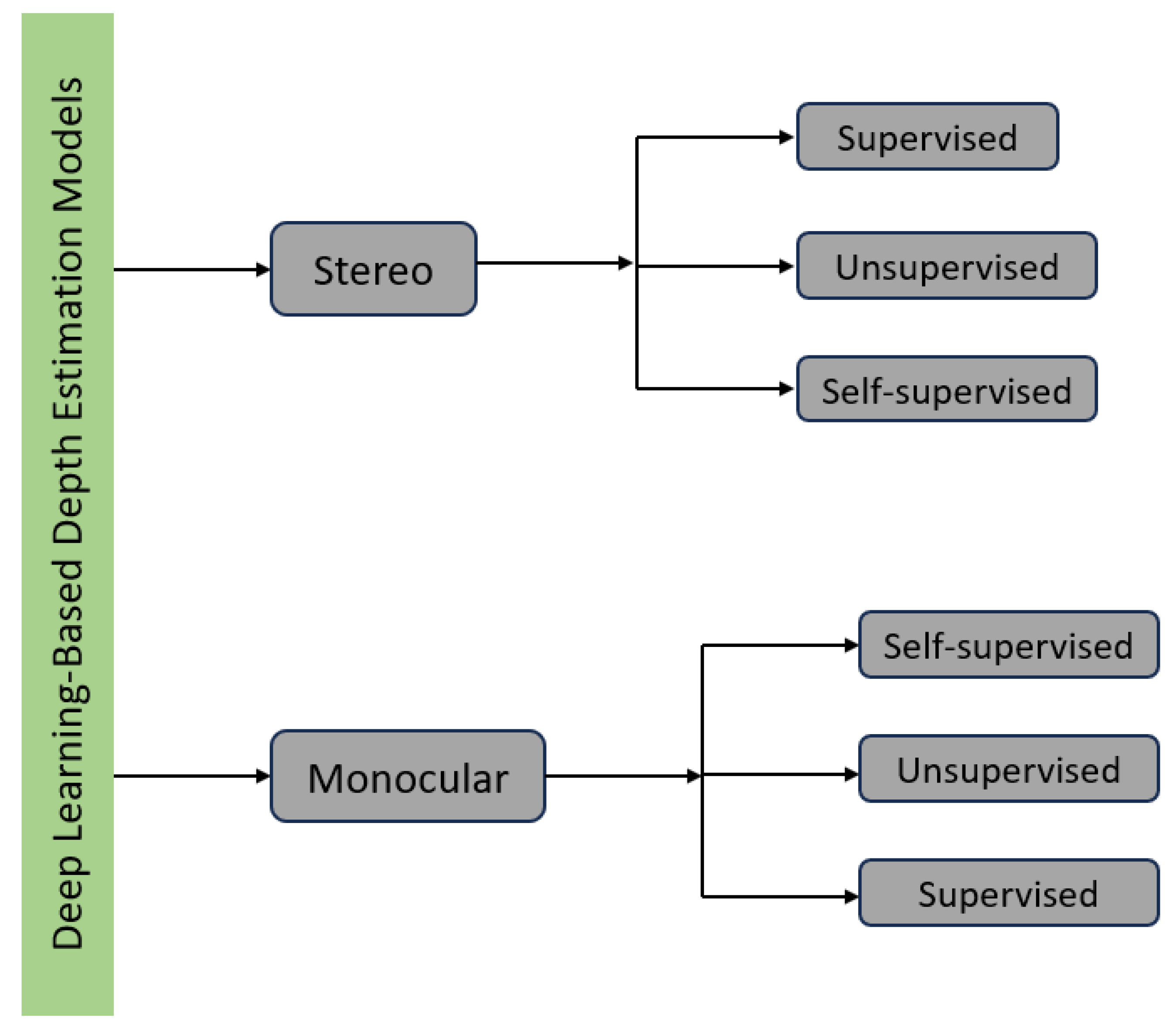
3. Taxonomy—For the Deep Learning-Based Depth Estimation Models

The depth estimation algorithms, both stereo and monocular, can be trained using the already available labeled ground-truth depth maps on datasets like Scene Flow (supervised models) or unlabeled RGB images (self-supervised or unsupervised models) as shown in Figure 1. The merits and demerits of these training modes are depicted in

Table 1. Merits and demerits of various modes of training.

Training Modes	Merits	Demerits
Supervised	Training on ground truth-labeled data provides the algorithm with a prior understanding of the scene. Accuracy is high when evaluation data show limited variation from training data.	Training is time-consuming. Ground-truth data are not easily available. Requires pre-training multiple times to be generalized to varied datasets.
Unsupervised	Does not require ground truth-labeled data to be trained on. Well generalizable to new datasets and unseen environments.	Requires relatively more computational time than supervised methods. Generally, less accurate than supervised learning methods.
Self-supervised	Does not need ground truth-labeled data for training, but model labels the data. Good generalizability across varied datasets.	Needs much more computational time as compared to supervised methods. Generally less accurate than supervised learning models but better than unsupervised models.

. The algorithms are classified according to the modes of training used for their performance, as demonstrated further in the paper. The training modes for the algorithms are explained in this paper with corresponding diagrams.

These core components of deep learning-based depth prediction models have three phases: training, validation, and prediction. The learning types have similar validation and prediction phases, but they mostly vary in their training phases. The overall learning mechanism is demonstrated in Figure 2.

The training phases of the three learning methods are depicted in the figure below and explained accordingly.

Supervised learning, the training phase of which is shown in Figure 3a, is the most common type of training method that has been used for deep learning-based techniques. Here, the pair of input labels is given. Then, in this approach, a deep network (like a Convolutional Neural Network) is trained directly with the help of the labels to give an output in the form of the prediction of the label from a given image in the testing phase. It also evaluates a loss, which is differentiable, between the predicted and the actual answer. Through the network, it also backpropagates to update the weights for prediction optimization. In general, the supervised type of learning has been the most acceptable form of learning since the assumption is that the labels of every image will be given, which is a factor to ease up the whole learning phenomenon for the network.

Unsupervised learning, the training phase of which is shown in Figure 3b, involves the network learning process with input images without any kind of labels, using the concept of clustering to find a pattern. Given some data, the network finds features that are similar in nature and then groups them. K-means and K-medoids are some of the methods followed in clustering. Such clustering technique helps in giving an output that has relevance concerning the groups formed during clustering. This helps in the high generalizability of the method over the supervised one.

Self-supervised learning, the training phase of which is shown in Figure 3c, follows the ideology of the unsupervised learning method, in the sense that even in this case, the input images are without labels. However, in place of using the concept of clustering, this method attempts to handle the issue using tasks used by supervised learning methods, like classification and regression. Numerous research lately has brought this method to fruition using the technique of learning in a contrastive manner to the positive and negative pairs. Images are labeled as positive and negative pairs based on the augmentation technique used. The network then draws the positive features away from the negative ones. Thus, images of like classes are grouped. This helps tasks, like classification, be possible without the need for any labels or ground truth.

4. Stereo Depth Estimation Methods

4.1. Supervised Stereo Models

Due to the recent advancements in the realm of Convolutional Neural Networks (CNNs), stereo-depth estimation has been demonstrated as a supervised learning problem. Such deep learning approaches have proven to transcend traditional techniques in terms of performance. However, one of the major demerits of CNNs, which is the extraction of context features and other information from ill-posed areas, has been innate in the deep learning techniques for a long time. Thus, the generation of fine-quality disparity maps for the ill-posed regions is the prevalent problem that has been targeted and solved in “Cascade Residual Learning: A Two-stage Convolutional Neural Network for Stereo Matching” [38]. As its contribution, the end-to-end trained CRL (Cascade Residual Learning) scheme joins the pipeline from matching cost evaluation to disparity refinement using non-linear layers to demonstrate that residual learning provides better refinement as compared to direct disparity learning at a stage. The CRL network is a CNN architecture of the cascaded type with two stages—in the commencing stage, DispFulNet, a suggested DispNet [33], is equipped with additional up-convolution modules to produce highly detailed disparity images. The second stage, DispResNet, corrects this disparity by joining with the first stage to produce residual signals across numerous scales. The conglomeration of the two-stage outputs yields the final disparity.

Figure 4 depicts the architecture of the CRL network. The first stage, DispFulNet, has the left and the corresponding right stereo images ($L_i$ and $R_i$, respectively) as inputs to generate the initial disparity regarding the left image ($d$). The right image is then warped following the disparity to obtain the left image of the synthesized form $(L_i^{’}$).

$$L_i^{’}(x,y)=R_i(x+d\left(x,y\right), y)$$

(1)

Thus, the second stage, DispResNet, has the input of $L_i$, $R_i$, $d$, and $L_i^{’}(x,y)$ and the error $err$. The error is depicted as follows:

$$err=|L_i-L_i^{’}\left(x,y\right)|$$

(2)

With the first stage providing the initial disparity, the next stage gives the respective residual signal. The new disparity is given by $(d+r^{’})$. The residual signals are produced across multiple scales, with the scale ranging from $0$ to a value of $S$ ($0$ denotes the full-resolution scale). The final disparity, after down sampling the initial disparity, at scale $s$ is given by,

$$d^{’\left(s\right)}=d^s+r^{’\left(s\right)}, s ϵ [0,S]$$

(3)

where $d^s$ and $r^{’\left(s\right)}$ denote the initial disparity and the residual signal corresponding to the initial disparity, respectively, at scale $s$.

The disparity images at full resolution, from the output of the DispFulNet, with other intermediate ones, are supervised using the ground truth by evaluating the L1 loss. For the supervised learning paradigm of DispResNet, again an L1 loss is evaluated between the estimated disparity and the ground-truth disparity at every scale. To implement the CRL model, the Caffe framework [39] is made use of. The model is essentially trained in FlyingThings3D and in KITTI 2015. The parameters of [33] are used while training the first or the second stage on the FlyingThings3D dataset. However, some model architectures depend upon patch-based Siamese networks, which have similar demerits regarding finding correspondences in certain regions. To address such identical issues in “Pyramid Stereo Matching Network” [40], the problem targeted was to extract and use context information to find correspondence in regions that are ill-posed. The end-to-end PSMNet (Pyramid Stereo Matching Network) contributes to the approach differently and without any post-processing. The pyramid stereo matching network contains a couple of modules: spatial pyramid pooling and a 3D CNN. The former gathers global context information, for incorporating into image features, of various scales and positions to form a cost volume. The stacked hourglass 3D CNN learns to regularize the cost volume with stacked multiple hourglass networks along with supervision at intermediate stages.

Due to the use of disparity regression for continuous disparity map estimation, the smooth L1 loss function is used to train the suggested network. This loss is used in bounding box regression to detect objects due to their robustness and low sensitivity to outliers. This model is trained on the Scene Flow dataset with dense ground-truth disparity maps. The architecture is implemented with PyTorch and the Adam optimizer is used to train the network end-to-end. Four NVIDIA Titan-Xp GPUs were used for the training phase. The depth maps produced by the various methods were satisfactory in the sense that they could serve their purpose of estimating the distance of the objects from the reference point, generally from the camera, with appreciable accuracy. However, to augment the horizon of application, edge detection is a concept that has been demonstrated in the depth estimation model of “StereoNet: Guided Hierarchical Refinement for Real-Time Edge-Aware Depth Prediction” [41]. It is an end-to-end deep network model that produces fine-quality, quantization-free, and edge-manifested disparity maps. This network obtains sub-pixel matching accuracy which is relatively higher, compared to the traditional approaches. This allows for attaining precision of the traditional stereopsis with a low-resolution cost volume. It also shows the over-parameterization of the previous work and how it appreciably reduced the run-time of the system. It even contributes to the establishment of a hierarchical depth-refinement layer which performs fine up-sampling for edge preservation. The Siamese network is utilized for feature extraction from both the left and right images.

A hierarchical layer for refining depth is implemented, which performs high-quality up-sampling for preserving the edges. For the training of the network, the fully supervised mode is followed with the ground truth-labeled stereo data. The hierarchical loss function is minimized, and it represents a smoothed L1 loss. The network is initially trained on the Scene Flow dataset. Tensorflow is used to implement and train the network, and the experiments are optimized using RMSProp (Root Mean Square Propagation) [42]. It runs at 60 fps on a high-end NVIDIA Titan X GPU. Another edge-preserving end-to-end deep network, EdgeStereo from “EdgeStereo: A Context Integrated Residual Pyramid Network for Stereo Matching” [43], is capable of multi-tasking and is comprised of the basic disparity network and a sub-network to preserve the edges. The edge cues and edge-aware loss guide the disparity learning. The context pyramid and the residual pyramid are established, which help in dealing with the ill-posed areas and in replacing the cascade refinement structures, as a contribution of the model. This model enables predicting, from a stereo image pair, both a disparity map and an edge map.

To include context information in the multi-scale mode in the disparity branch, a context pyramid is established initially, after which a residual pyramid of the compact type is developed for cascaded refinement. To preserve the nuanced details of the edges, this model embeds boundary features and regularization of the edge-aware smoothness loss function. Edge detection helps enhance stereopsis. The training part is split into three phases to allow for multi-task learning for the model. In the initial phase, the sub-network for edge detection is trained on a dataset and a cross-entropy loss of the class-balanced type, demonstrated in [44], guides it. In the second phase, deep supervision is used for the supervision of regressed disparities across various scales on a dataset for stereo vision.

The total loss is the sum of the losses at the concerned scales. Along with the smoothness loss for the disparity, the regression loss for supervised learning is also included. In the final phase, every layer of the model is optimized on a single dataset used in the previous phase. Again, deep supervision is used across the scales. The only constraint used in this phase is the avoidance of using the edge-aware smoothness loss function since the edge contours used in the previous phase have greater stability than those used in the final phase. The model is trained on the Scene Flow dataset with dense ground-truth depth maps. To pretrain the sub-network for edge-detection, the BSDS500 [45] dataset is considered. Going along with [44,46], the data for training in BSDS500 is combined with the PASCAL VOC Context dataset [47]. Based on Caffe [39], the implementation of this model is carried out, and the Adam optimizer [48] is used to optimize it.

Such ideas of generating a final depth map for the application of autonomous driving are appreciable. However, some areas which require fast generation of these maps, irrespective of the precision, could incur a loss. Such areas include drones which might have to fly at high speeds at times.

For such domains, researchers have thought about the idea of the fast production of depth maps with low accuracy, which, in stages, will have the resolution of the maps enhanced gradually. This concept is generally used for obstacle-evasion and the final high-resolution maps can be used for trajectory generation for flying objects. With such a concept in mind, a network, AnyNet, has been proposed in “Anytime Stereo Image Depth Estimation on Mobile Devices” [49] to predict disparity in the anytime setting. This method trades the time of computation and precision whenever needed during inference. Depth estimation takes place in stages and the model produces the current best output whenever commanded to do so. Much lesser parameters are needed than many recent approaches to produce disparity maps with appreciable precision. This effectuates the usage of such models in embedded devices with constrained resources.

Finally, a spatial propagation model (SPNet) further enhances the quality of the disparity map. The full network is trained end-to-end with a joint loss over each scale, and the network is termed an Anytime Stereo Network (AnyNet). This network is implemented in PyTorch and trained end-to-end with the help of the Adam optimizer [48]. Following training on the Scene Flow dataset, the model is pre-trained on the same dataset for KITTI. One GTX 1080Ti GPU was used during the training phase of the model. Another domain in stereo depth estimation dealt with stereopsis on fine-quality images, which is not so easy to find. This concept is elucidated in “Hierarchical Deep Stereo Matching on High-resolution Images” [50]. To address the issue of stereo matching on high-resolution images in real-time due to limited processing speed and memory constraints, an end-to-end framework has been developed which looks for correspondences progressively following the route of a hierarchy going from coarse to fine mode. Since datasets dealing with high-resolution images are difficult to obtain, a couple of fine-resolution datasets are collected, and a dataset has been introduced containing stereo pairs of such fine resolution for training and evaluation. This design permits the generation of disparity as and when needed. It implies that any time setting is possible considering the intermediate results of disparity for close-range objects, with less latency of about 30 ms. Also, to enhance the robustness of the model to various factors, a set of augmentation strategies are developed.

In the training phase itself, the network is trained to predict at various scales, which allows for any time setting at any pyramid level and regularizes the overall network. At each level, for the progressive disparity resolution, the losses are scaled. Pytorch is used for the implementation of the HSM network, and the training is performed using the Adam optimizer with four Titan X Pascal GPUs. HR-VS, a synthetic dataset, is developed and used to train stereo models of fine resolution. Middlebury, ETH3D [30,33,51], KITTI 2015, and HR-VS are enhanced, during the training phase, to be of equal size to Scene Flow, yielding about 170k samples of training. For the stereo-matching techniques dealing with the CNN form of deep learning, cost volumes help obtain significant precision in correspondence matching. MCV-MFC (Multi Level Cost Volume and Multi-Scale Feature Constancy) in “Stereo Matching Using Multi-level Cost Volume and Multi-scale Feature Constancy” [52] is such a CNN which can be trained end-to-end and focuses on the usage of cost volumes to their fullest extent for precise stereo depth estimation. It consists of three sub-modules: feature extraction, which is in shared mode, commencing estimation of disparity, and finally, refinement of disparity. Both the accuracy and the computational efficiency are enhanced by fusing the disparity estimation and refinement tasks into a single network. Multi-level cost volume evaluation is introduced, for which the feature discriminability is improved by considering information from various factors. The model robustness is also improved by introducing a finetuning scheme comprising a couple of stages.

Feature constancy of the multi-scale type is used for measuring the commencing disparity correctness in the feature realm for augmenting the disparity refinement efficiency. The tight coupling of the sub-modules makes it easy to train them due to their compactness. The model is robust enough to have the generalizability of considerable performance across various datasets. For this, a bi-stage strategy to finetune is demonstrated for the transfer of the model to the desired datasets. Here, L1 loss is used as the loss function to evaluate the average of the absolute difference between the disparities which are predicted and the ground truth. This average of the absolute difference itself is termed as the end-point-error (EPE). The stereo images and the respective ground-truth disparity maps are used for training the network on the Scene Flow dataset. However, training is also carried out on datasets other than Scene Flow for this model. CAFFE [39] was used for the implementation of the model and the ADAM solver [48] was used for its optimization.

Regarding multi-view stereo methods, the learning-based ones proved promising. Notwithstanding, they fail to consider the difference in visibility among the various views. This leads to an unsystematic creation of platforms for multi-view similarity prediction and limits their ability to work on datasets with robust variations in viewpoints. PVSNet in “PVSNet: Pixelwise Visibility-Aware Multi-View Stereo Network” [53] has been suggested for performing 3D reconstruction of the dense and robust type. It is a pixelwise visibility network to comprehend information related to visibility for the various neighboring images prior to evaluating the multi-view similarity. Two-dimensional visibility maps are regressed from two-view cost volumes. Due to the representation of undesirable image characteristics by the visibility maps, the regression permits the accepted views to have more weight in the eventual representation of cost volume. To add to it, a strategy to train the network to adapt to noises has been demonstrated which includes views which are disturbing during the training phase to increase the generalizability of the network to various unrelated views.

The L1 loss function is used for the training of the network. Two modes of training loss functions are included: the training loss for low-resolution prediction and one for high-resolution prediction. As suggested by [54,55], the DTU dataset [56] is classified into sets for training, validation, and finally, evaluation. The network is trained on the training set and the Poisson surface reconstruction [57] is used to produce depth maps for ground truth at some resolutions. The network implementation is carried out using PyTorch [58] and the RMSprop optimizer is used for network training on a couple of NVIDIA GTX 1080Ti GPUs. Unlike a few neural network stereo depth estimation techniques, as mentioned above, dealing with a full cost volume and depending upon 3D convolutions, the HITNet model in “HITNet: Hierarchical Iterative Tile Refinement Network for Real-time Stereo Matching” [59] depends on a quick multi-resolution step for initialization, a 2D geometric propagation which is differentiable, and some mechanisms for warping. Hence, this model does not develop any explicit cost volume. As its contribution, it consists of a swift multi-resolution initialization step that uses learned features to deal with fine resolution matches: a 2D disparity propagation stage which efficiently exploits the concept of slanted support windows with learned descriptors. Thus, it delivers with relatively less computation. End-to-end training of the network is carried out with ground-truth disparities with the help of the losses, namely an initialization loss, a propagation loss, a surface slant loss, and a loss to supervise the confidence.

The architecture of the model is represented in Figure 5. The module to extract features is based on a small U-Net [60]. The features contain details of the images in the multi-scale mode. After the feature extraction, initialization of the disparity maps is started at various resolutions as fronto parallel tiles. For that, a matching component evaluates several hypotheses and decides upon that with the lowest distance between the left and the right views of the feature maps. This output is then sent to the stage of propagation which refines the predicted disparity in a hierarchically iterative fashion, using the concept of slanted support windows.

The target of the initialization stage is to bring out an initial estimate of the disparity $d_i$ and a learnable tile-wise feature vector $p$ regarding the resolutions. The output of this stage is the disparity hypotheses having the form $h=[d, 0, 0, p]$. Basically, the feature maps are generated with tile-wise features ${\tilde{f}}_{r,x,y}$. The matching cost $c$ at location $(x,y)$ and resolution $r$ with disparity $d$ as

$$c\left(r, x, y, d\right)=\left|\right|{{\tilde{f}}^L}_{r,x,y}-{{\tilde{f}}^R}_{r,4x-d,y}\left|\right|$$

(4)

Subsequently, the initial disparity is evaluated; thus,

$$d_{r,x,y}^i={argmin}_{dϵ[0,D]}c\left(r, x, y, d\right)$$

(5)

for each $\left(x,y\right)$, where $D$ is the maximum value of considered disparity. Another approach, RAFT-Stereo in “RAFT-Stereo: Multilevel Recurrent Field Transforms for Stereo Matching” [61], similarly avoids the high computational memory consumption of 3D convolutions. It can be directly implemented for megapixel images with no resizing or processing needed for the image in patches. The main contribution of this work is that it has a different take on stereopsis, fusing stereo and optical flow techniques. It exhibits relatively better cross-data generalization, which leads to its high precision. It solely utilizes 2D convolutions and a light-weight cost volume. It is an architecture, conforming to the rules of deep learning, for a rectified mode of stereopsis and is inspired by RAFT [62], the optical flow network. Multi-level modes of convolutional GRUs are implemented which help in efficient communication of information signals across the concerned image. A merit of the network is that it up-samples the stereopsis at the final stage, making the network highly memory efficient, which, in turn, enables full-resolution stereo prediction on megapixel images.

The network is pretrained on the Scene Flow dataset [33]. The implementation of the network is carried out in Pytorch [63] and the training happens with the help of a couple of RTX 6000 GPUs. During this phase, the AdamW [64] optimizer is made use of. The experiments, excluding the ablation ones, are trained with the help of data augmentation. To enhance the zero-shot generalization performance, the additional versions of this network are trained with the help of additional data of the synthetic variety from datasets such as Tartan Air, Falling Things, and Sintel-Stereo. Considering the demerits of CNNs, yet another disadvantage of the appreciable computational time consumption, which slows down the inference generation, has been addressed in “CRAR: Accelerating Stereo Matching with Cascaded Residual Regression and Adaptive Refinement” [65]. Although some of the previous works solved this issue by down sampling the input images to reduce the spatial size, this augments the rate of errors. The method of CRAR accelerates the algorithms for stereo matching by improving the structure of the network. It decreases the number of features which have a direct proportionality with the computational cost. This cost aggregation, due to its extra dimension while using the 4D feature manipulation technique, is the most time-consuming factor of some of the stereo-matching methods. Based on the concept of compressing a network, decomposition and sparsification are carried out to squeeze the network for cost optimization since it is computationally expensive. The various refinement methods used earlier have been combined to establish a consolidated algorithm to execute parallelism for running required devices to accelerate the inference even further. The smooth L1 loss function is used for the training of the network. Experiments are carried out using PyTorch, and the optimization of the network is performed with the help of the Adam SGD optimization procedure. According to the works of [40,66,67], the network is pretrained on the Scene Flow dataset.

Some research works focused on developing the cost volume with a well-performing depth estimation model. Their idea was that a compact but information-manifesting cost volume is necessary for precise and efficient stereo matching purposes. In “Attention Concatenation Volume for Accurate and Efficient Stereo Matching” [68], a method to construct cost volume has been demonstrated which uses clues of correlation to obtain attention weights to augment the information relevant to matching. The concept of patch matching of the adaptive type and of multiple levels has been used to demonstrate the high reliability of the weights. These all happen in the concatenation volume and help highlight the uniqueness of the cost at various disparities also for the regions being ill-posed. The suggested cost volume is termed as Attention Concatenation Volume (ACV), which can be implemented in many stereo methods. The core contribution of this paper focuses on the usage of the informative and efficient cost volume representation using the similarity details stored in the correlation segment; this is to regularize the concatenation volume for the demand of a lightweight aggregation network to attain significant efficiency and precision.

The smoothness loss is used as the final loss for the network. The model is implemented using PyTorch and the training is conducted on NVIDIA RTX 3090 GPUs. The Adam optimizer is used for every experiment. Another project worked on improving the robustness of an already existing method of stereopsis. Robustness is unavoidable since eventually the depth estimation methods are applied to real-time cases. Unlike the common lengthy procedures, the following paper asserts that gathering numerous datasets for training is an easy way of enhancing the generalization ability of the algorithms. The paper “An Improved RaftStereo Trained with A Mixed Dataset for the Robust Vision Challenge 2022” [69] provides an improved version of the RaftStereo [61] and the model is trained with an eclectic dataset containing seven datasets for the purpose of the Robust Vision Challenge. It is termed as the iRaftStereo_RVC. The datasets used are Sceneflow, CreStereo, Tartan Air, Falling Things, Sintel-Stereo, HR-VS, and InStereo2K. The amalgamated form of the above datasets is used to pre-train RaftStereo before its fine-tuning is carried out.

The experiments are carried out with the open-source code of RaftStereo being implemented using Pytorch. For training, a couple of RTX 2080Ti GPUs are used. However, with the cross-domain generalization capability of such an algorithm enhanced, its stereo matching performance has a good probability of being degraded. To deal with the trade-off between the performances based on stereo-matching and cross-domain generalization, “PCW-Net: Pyramid Combination and Warping Cost Volume for Stereo Matching” [70] suggests a network, PCW-Net (Pyramid Combination and Warping Network), based on cost volume related to combination and warping to achieve significant results from both types of performances on varied benchmarks.

The paper contributed to an effective framework which attained significant generalizability from synthetic to real-time datasets and, after fine tuning, performed appreciably on target datasets. A cost volume fusion module of the multi-scale type is developed to act according to receptive fields of the multi-scale category and bring out structural cues which are domain independent. This leads to better stereopsis of varied image resolutions. A warping disparity refinement segment which is efficient and volume dependent is introduced, which eventually helps to find the appropriate residue in an uncontrolled environment.

The architecture of the model is depicted in Figure 6. It consists of three components: the component to extract features in multi-scale mode, the cost-aggregation component based on the combination volume of the multi-scale mode, and the component to refine the predicted disparity based on the warping volume. The features, after being extracted, are used to establish a pyramid volume. Combination volumes are then developed on the top pyramid levels, and then a fusion module for the cost volume is developed to fuse them for the commencement of the disparity estimation. Eventually, at the final level, the warping volume is established to refine the estimated disparity.

In the feature extraction component or module of the multi-scale mode, with a pair of images as input, three convolutional layers are used for obtaining the unary feature map at the initial level. Subsequently, three residual blocks are implemented to obtain the feature maps at the next three levels. Using the features extracted, pyramid cost volumes are established at various stages. In the cost-aggregation component, the combination volume is established at four levels. For every level, $l$, the combination volume, $V_{com}^l$, includes the volume for concatenation, $V_{conc}^l$, and the volume for group-wise correlation, $V_{gcorr}^l$. Considering the feature extracted at each level is $f^l$, the combination volume is evaluated as

$$\begin{gathered} V_{com}^l=V_{conc}^l\left|\right|V_{gcorr}^l \\ {V}_{conc}^l\left(d, x, y\right)={\delta }_1\left(f_L^l\left(x, y\right)\right)\left|\right|{\delta }_1\left(f_R^l\left(x-d, y\right)\right) \\ {V}_{corr}^l\left(d, x, y, g\right)=\left(1/\left(n_c^l/n_g\right)\right)〈{\delta }_2\left(f_L^{lg}\left(x, y\right)\right),{\delta }_2\left(f_R^{lg}\left(x-d, y\right)\right)〉 \end{gathered}$$

(6)

where $\left|\right|$ represents the operation of concatenation at the axis of features, and $f_L^l$ and $f_R^l$ denote the features extracted for the left and right images, respectively. $f^{lg}$ denotes the features which are grouped and are symmetrically divided from the extracted one, $f^l$, considering the number of groups as $n_g$. $d$ stands for the disparity levels. $n_c$ denotes the channels of $f^l$, and $〈,〉$ denotes the inner product. During the establishment of the combination volume, an extra convolution layer is included without the function of activation and batch normalization (normalization layer $\delta$) to have $f^l$ and $f^{lg}$ with identical distribution of the data. The multi-scale combination volume is fused together to estimate the disparity map at the initial stage.

In the cost-volume fusion, the combination volumes, encoder blocks, followed by blocks for fusion and decoding are represented by ${Vol}^l, {En}^l, {Fs}^l \mathrm{a}\mathrm{n}\mathrm{d} {De}^l$, respectively, where $l ϵ \left[1, 4\right]$ represents the levels. The ultimate fused cost volume is $D_{O/P}$. After that, a few 3D hourglass networks are stacked to finally generate the commencing disparity map $d_l$. The suggested blocks for fusion have a couple of main inputs—the encoder blocks, which deal with the cost-volume of high resolutions, and the combination volume, which helps evaluate the similarity between the left and the corresponding right features. The process is formulated as

$$F_s^l=Conv\left({Vol}^l\left|\right|{En}^l\right)$$

(7)

where $Conv\left(\right)$ denotes the layer of convolution. The encoder and decoder processes are then developed. In this model, regarding the component for refining the predicted disparity, an input of the multi-modal variety is used to help the network learn the residue and consists of the warping volume, which is 3D in nature, the commencing disparity map, the left features, and the reconstructed error. In the volume for warping, the left feature and the warped right feature are implemented to establish this volume at the final level. The predicted initial disparity, $D_{in}$, is referred to while warping the right features. The residual disparity is considered small and, hence, a tiny search range, $d_r$, for the residue is implemented. The warping volume is evaluated as

$$\begin{gathered} V_{warp}\left(d_r, x, y\right)=\left(1/n_c\right)〈f_{unl}\left(x, y\right), f_{warp}\left(x-d_r, y\right)〉 \\ {f}_{warp}=warping\left(f_{unr}, D_{in}\right) \end{gathered}$$

(8)

where $f_{unl}$ and $f_{unr}$ are unsampled from the initial feature level to the actual size of the image. Subsequently, the concept of a reconstructed error helps to identify flawed regions of commencing disparity prediction and is evaluated as

$${err}_{rc}=f_{unl}\left(x, y\right)-f_{warp}\left(x, y\right)$$

(9)

With this, the refinement network better recognizes the pixels to be optimized further. The left features and the initial disparity map are amongst the inputs to the refinement network. The initial disparity gives a base to the network to carry out more optimization operations, and the feature of the left image possesses context for learning the residues. For weight balancing of the input, the commencing disparity is regularized by a layer of convolution.

Drawing inspiration from the previous works of [40,71], the smoothness loss function is used for training the network in an end-to-end fashion. The suggested framework is implemented using Pytorch and trained using the Adam optimizer. The training of the experiments was carried out on a couple of NVIDIA V100 GPUs. Another model which can simultaneously achieve appreciable performance in real-time with a high level of precision and high generalizability is the one suggested in “CGI-Stereo: Accurate and Real-Time Stereo Matching via Context and Geometry Interaction” [72]. The crux of the model is a fusion block which helps fuse information related to context along with geometry for precise and efficient cost aggregation. It also gives feedback to feature comprehension to help extract highly effective contextual features. The suggested block can be implemented in various methods of stereo matching. A different design of cost volume is introduced to consider information related to both matching and content. A compact and informative cost volume has also been suggested, which leverages a correlation volume for filtering a feature volume. Based on the fusion block and this compact cost volume, the model is developed.

The network is trained in a supervised manner and in an end-to-end fashion using the smoothness loss. PyTorch is used for the implementation of the method and the experiments are performed with the help of NVIDIA RTX 3090 GPUs. The Adam optimizer is used for the experiments.

4.2. Unsupervised Stereo Models

Sometimes obtaining the ground-truth depth data can be troublesome; due to this, a shift to unsupervised depth estimation techniques has gained attention over the past few years. Due to the lack of ground-truth data, the geometric and photometric consistency constraints are generally used as the main supervisory signal in the unsupervised techniques. The recent deep MVS (Multi-View Stereo) methods have presented significant improvement in their performance. However, they rely on ground-truth depth maps for supervision, acquiring which is not an easy task. Hence, in “Learning Unsupervised Multi-View Stereopsis via Robust Photometric Consistency” [73], novel view images are used solely as signals of supervision for the designed framework to enable the comprehension of unsupervised stereopsis of the multi-view category. The photometrically consistent reprojections, provided by geometry, are used to minimize the equivalent reprojection error, which is implemented for the training of the CNN of the model. Basically, a photometric consistency loss of the multi-view mode and robust nature is used to learn unsupervised depth prediction, which then permits overcoming occlusions and changes due to lighting across various views of training.

The ADAM [48] optimizer is used during the training of the network. To implement the pipeline of the learning model, Tensorflow [74] is used. As stated by [55], the appreciable efficiency of the model is maintained using a small image resolution and coarse depth steps, due to the elevated requirements of the GPU memory, during training. However, during the evaluation, the settings can be increased to higher modes. Similarly, supervision with the help of ground-truth data can impede the generalization of the learned models in unexpected scenarios. In “MVS²: Deep Unsupervised Multi-view Stereo with Multi-View Symmetry” [75], an end-to-end deep MVS network of unsupervised learning is suggested that can be learned with no use of ground-truth depth as a signal for supervision. The photometric consistency across the various views, in the form of image warping errors of the multi-view mode, suffices in training the network for converging to the desirable state which enhances the performance. It contributes to the introduction of the cross-view consistency in depth prediction and the proposal of a loss function for consistency measurement. This, in turn, is implemented to train the deep network. This network also learns the occlusion maps of the multi-view mode. This enhances the network robustness to deal with real-time occlusions.

The implementation of the MVS² network is conducted in Tensorflow with an NVIDIA v100 GPU. The DTU training dataset is used to train the model. “Progressive Fusion for Unsupervised Binocular Depth Estimation using Cycled Networks” [76] is yet another trainable end-to-end unsupervised deep network with regard to estimating depth based on adversarial learning. It contributed to the introduction of a novel Progressive Fusion Network (PFN) which combines the information from both images of a stereo pair and is developed on a multi-scale refinement technique. The process is customized according to the couple disparity maps predicted by the PFN. To have the form of a cycle, the sub-network is stacked twice. The arrangement gives strong constraints and, hence, supervisory signals for each view of the image. This allows for network optimization. This form manifests as a data-augmentation type. This is because while training and after learning, the disparity maps are predicted by the network from the training images, which happens in the forward pass of the cycle, and from the images which are synthesized, which happens in the backward pass of the cycle. To add to it, in the forward pass of the cycle, deformed or blurred images are prevented from being predicted by the sub-network or there would be ramifications for them in the backward pass of the cycle. There is joint learning in the whole cycle. The initial network provides the end disparity map.

For training, the reconstruction loss, the consistency loss, and a least-square GAN loss [77] are used. For the optimization of the network, the Adam optimizer is made use of. The training happens on a couple of Titan Xp GPUs. For the implementation of the suggested model, TensorFlow is utilized. Similarly, in “M³VSNet: Unsupervised Multi-metric Multi-view Stereo Network” [78], a multi-metric MVS network, M³VSNet, of the unsupervised type is introduced which works even in real or non-ideal environments and infers depth maps for the reconstruction of dense point clouds. An innovative multi-metric loss in the form of the pixel-wise and feature-wise loss function includes the varied correspondence-matching perspectives happening beyond pixel value. Concerning the loss function, the geometric as well as the photometric matching consistencies are assured to be both high and robust relative to MVSNet’s sole photometric constraints. Other than that, to enhance the continuity and the precision of the generated depth maps, the consistency of normal depth is included in the format of the 3D point cloud.

Pytorch is used for the implementation of the network. For training, the training set of DTU is solely utilized, which has no ground-truth depth maps. Four NVIDIA RTX 2080Ti and the ADAM optimizer are used for the training of the model. Despite the development of the unsupervised methods, the depth maps generated are of low resolutions due to the memory consumption of the processes. In “Unsupervised multi-view stereo network based on multi-stage depth estimation” [79], an innovative unsupervised network of the multi-view mode has been demonstrated which can enhance the resolution of the depth map and help in the generation of a detailed dense 3D model. To enhance the resolution of depth maps by reducing the cost volume memory consumption, multiple stages of the progressive coarse-to-fine type are considered. A multi-view correlation based on groups is established to minimize the irrelevant insights in the channel-wise dimension, and a correlation prior to the multi-view category is also demonstrated.

The pixel-wise photometric consistency for certain views is implemented to reduce the repercussion of occlusion and reflection. For augmenting the robust nature of the model, the structure loss, including structural similarity, has been implemented. To maintain the smoothness of the estimated map, the depth gradient smooth loss has been considered too. The overall loss function is the combination of these stage losses with the concerned weights. Several techniques based on pseudo labels are brought up to emphasize the constraint of the loss function, owing to the weakness of the supervision signal of the MVS method with the unsupervised mode in intricate areas. Numerous training processes are involved in such techniques and extra supervision signals like optical flow or the established depth map of the mesh model being reconstructed are presented. To produce this optical flow for supervision as an extra one, PWC-Net [80] is applied in the commencing level of U-MVSNet [81].

The method is implemented using the PyTorch framework on four TITAN-RTX GPUs. The Adam optimizer is used to optimize the network and the regularization is performed using SGDR [82] to prevent the convergence of parameters to the local lowermost level. Another deep learning-based unsupervised network, “H-Net: Unsupervised Attention-based Stereo Depth Estimation Leveraging Epipolar Geometry” [83], is suggested to erase the dependency on supervised learning schemes. The framework is of the end-to-end type, which makes meritorious utilization of epipolar geometry for the stereo-matching process. An encoder-decoder architecture of the Siamese type in the self-supervised mode is introduced which augments the ease of communication between the left and right images mainly by combining their complementary information. The mechanism of the mutual epipolar attention concept is developed to include the epipolar constraint in feature matching. The correspondences of features, lying on a single epipolar line, are signified by the mechanism as it comprehends the information which is mutual between the stereo pair given as input. Semantic information is also included in the suggested mechanism of the attention concept to further augment the correspondences in the stereo matching process. Furthermore, the concept of attention is subdued, and the outlier errors are removed in the areas invisible to both cameras by deploying the optimal transport algorithm.

The consistency between the input images and their corresponding reconstructed ones gives the signal for supervision. A function for the photometric error has been used which contains the L1-norm along with the index for structural similarity. To enhance the predictions of the boundaries, an edge-based smoothness component has been implemented. Eventually, the photometric and the pixel-wise smoothness loss terms were balanced using a term for smoothness and the overall loss was evaluated. The PyTorch library was used to train the network, using the Adam optimizer, on a single NVIDIA 2080Ti GPU.

4.3. Self-Supervised Stereo Models

The lack of labeled ground-truth disparity also obliged the evolution of the self-supervised method of learning, where the model is basically responsible for giving labels to the data, creating pseudo-labels from the data themselves. These models can be argued to be relatively more prevalent because, generally, they are easier to evaluate than the unsupervised models. In “Light-weight network for real-time adaptive stereo depth estimation” [84], considering the self-supervised method of learning for online adaptive stereopsis for both low GPU memory space and low computation cost, a lightweight adaptive network (LWANet) is presented for real-time stereopsis. A 3D convolution of the pseudo type appreciably minimizes the computational cost, with a slight compromise in accuracy, for which it is implemented in the cost volume aggregation portion. Other than that, to enhance the estimation of the eventual disparity, a U-Net architecture of high efficiency is fused with the CSPN [85] refinement module. It also contributes to industrial applications, providing them with a generalized depth estimation strategy. This method involves the amalgamation of the structural similarity index (SSIM) and the distance loss, which is termed as the photometric image reconstruction cost. Then, the gradient distance loss between the predicted disparity and the image of the left side is exploited to enhance the consistency of the edge. Pytorch is used for the network implementation, and for its training, NVIDIA 1080TI GPU is deployed. To update the parameters while training, the Adam optimizer is made use of.

Supervised multi-view stereo depth prediction techniques have achieved promising results with the training using ground-truth depth data. That being said, gathering multi-view depth data in large quantities is not easy. For this reason, a self-supervised strategy, “Self-supervised Learning of Depth inference for Multi-view Stereo” [86], is implemented for multi-view stereopsis which exploits, from the data as input, pseudo labels. Initially, depending on the reconstruction loss of an image as supervision, the model learns to generate initial pseudo labels under a learning framework of the unsupervised type. To leverage the information regarding depth inferred from high-resolution images and neighboring views, the initial labels are refined with the help of a punctiliously designed pipeline. Such high-quality pseudo labels are used as supervisory signals for the purpose of training the network and for its performance improvement by self-training, iteratively.

The base network in CVP-MVSNet (Cost Volume Pyramid-based depth inference from Multi-View Stereo) [87] is adopted because of its compactness and flexibility in dealing with fine-resolution images. The view synthesis loss of [75] and the perpetual loss of [88] are implemented to establish a strong relationship between the synthesized and the corresponding reference images. Finally, a weighted fusion of four loss functions, the image gradient loss, the structure similarity loss, the perpetual loss, and the depth smoothness loss, are made use of. For the same reasons, another self-supervised depth prediction network, SMAR-Net in “Self-Supervised Multiscale Adversarial Regression Network for Stereo Disparity Estimation (SMAR-Net)” [89], has been proposed to avoid using the ground-truth depth data for training. The network consists of a pair of stages. Disparity regression comprises the initial stage, where a network for regression uses stereo image pairs, which are stacked, to predict the values of disparity. There also exists a discriminator that assists in training the regressor. In the final stage, depending on the assumption of the left–right consistency, a synthetic left image is produced. To deal with real-time data, an image-warping operation is exploited.

The image stacking segment is proposed before extracting features and contains the spatial appearance of the stereo images and implies their matching correspondences with varied disparity values. Furthermore, a multiscale pooling layer is used to emphasize the consistency of object sizes and receptive fields. The model also predicts stereo disparity with features of the multi-scale variety in both the regression and discrimination segments. This combination helps predict disparity in ill-posed regions.

For the training purpose of the network, a hybrid loss function is minimized, and it consists of a content loss and an adversarial loss. The joint implementation of extraction of features, belonging to the multi-scale type, in both types of losses helps further enhance the generalizability of the network in the regions which are ill-posed. This network is implemented using PyTorch. Uniform distribution is used to initialize network parameters and ADAM is used to optimize them. The training of the network is carried out on a single Nvidia Quadro P5000 GPU. In the realm of surgeries assisted by computers, some of the intricate steps involve dense depth prediction and 3D reconstruction of any surgical scene. However, ground-truth data are not easily available for laparoscopic imaging and, in general, for supervised learning implementation of a stereo depth estimation model. Hence, a self-supervised method, SADepth (Self-supervised Adversarial Depth Estimation) in “Self-Supervised Generative Adversarial Network for Depth Estimation in Laparoscopic Images” [90], has been suggested to predict dense depth based on Generative Adversarial Networks. To consider geometry constraints during the phase of training, the network contains an encoder–decoder generator along with a discriminator. The adopted generative U-Net architecture benefits from the complementary information of the input stereo images. The photometric reprojection loss causes the local minima, which are solved with the help of the disparity smoothness loss, and the network of the multi-scale mode is formed. Adversarial learning helps enhance the quality of the generation of the framework.

Regarding the training, the structural similarity between the concerned actual images and the ones that are reconstructed is the supervisory signal for the training of the generator. In the network, the generator loss is formed using the appearance matching loss and the smoothness loss of disparity. The discriminator loss and the multi-scale losses are also implemented. Finally, the joint optimization loss is a conglomeration of the generator loss and the adversarial loss. PyTorch is used for the implementation of the model, and its training is carried out by the Adam optimizer and performed using a single NVIDIA 2080 Ti GPU. Similarly, another architecture, in “Self-Supervised Learning for Stereo Matching with Self-Improving Ability” [91], based on a CNN, has been designed which learns to estimate disparity maps of the dense type directly from the stereo inputs. The image warping error is used as the loss function to guide the process of learning. This network is well-generalizable to various unseen scenarios and to various settings of the camera.

With rectified left and right stereo images, $L_i$ and $R_i$, being given, the task of the network is to learn a function $f$ to predict pixel-wise disparity maps of the dense type, represented as $d_l=f(L_i, R_i)$ and $d_r=f(R_i, L_i)$ to be disparity maps for the left and right images, respectively. The function can be learned with the need for no disparity maps of the dense type, for which the stereo matching is formulated as a problem of warping of image. To be specific, if the left image $L_i$ and the disparity map corresponding to the right image $d_r=f(R_i, L_i)$ are obtained, the right image can be attained by the process of warping to be conducted on the left image regarding the dense disparity map, shown as follows:

$$R_i^{’}(x,y)=L_i(x+d_r\left(x,y\right), y)$$

(10)

where $R_i^{’}$ is the right image of the warped type. The inconsistency between the warped images and the observed images act as the supervisory signal in the learning of the function spoken above. For this mode, it is performed using a deep CNN in an end-to-end self-supervised manner. Figure 7 depicts the network architecture which has five modules: a module to extract features, module to generate cross feature volume, module for 3D feature matching, module to perform the soft-argmin operation, and the module for the warping of images. The module to extract features contains a set of residually connected 2D convolutions to bring out local features. The learned features are gathered into an assembly of a couple of cross-feature volumes. Subsequently, the feature matching module is used for mapping the 2D features to a higher dimension for distinction. Then, the soft-argmin is used to project the 3D volume to a 2D volume. In the final module, warping of images is performed to calculate the photometric error, which serves as the supervisory signal for the network training.

Basically, the learned features are used to construct a feature volume to evaluate the cost of stereo matching. The volume is constructed by exhausting the levels of disparity in a range already stated. If the feature maps brought out from the left and right images by the feature extraction component are represented as $L_f$ and $R_f$, the left-to-right feature volume at a position of the pixel represented by $(x,y)$ with disparity $d$ is given as follows:

$$F_{L-R}\left(x, y, d\right)=L_f\left(x, y\right) \left|\right| R_f(x-d, y)$$

(11)

Similarly, the right-to-left feature volume is given as follows:

$$F_{R-L}\left(x, y, d\right)=R_f\left(x, y\right) \left|\right| L_f(x+d, y)$$

(12)

The matching cost is learnt at each disparity with the photometric-based unary loss term and the local regularization. A module with a top-down approach is presented for better feature extraction. The output of this module is basically a 3D volume with features that are regularized. The step to match features are implanted in the 3D volume to 2D conversion stage since for warping, a disparity map of 2D is required. During the step, the dimension of disparity in the feature volumes is reduced by choosing the disparity with the least value of the distance between the corresponding left and right features. The soft argmin operation is performed over the disparity dimension for the 3D volume projection to its 2D version. The operation is given as follows:

$$argmin\sum _{d=0}^{D_m}d\times \sigma (-c_{e_d})$$

(13)

where $c_e$ represents the estimated cost (at disparity $d$), $D_m$ is the already stated disparity range, and $\sigma \left(\right)$ represents the softmax operation.

Under the self-supervised mode of learning for stereo matching, the image reconstruction error is used to decide upon the quality of the estimated disparity map. The loss function to learn to estimate the disparity map consists of a photometric-based unary term, a regularization term for the field of disparity, a constraint of consistency between the stereo pair of images and the corresponding maps of disparity, and finally, the maximization of depth heuristic (MDH) term. The network is implemented using TensorFlow. End-to-end optimization of the models is carried out using RMSProp. Another self-supervised deep learning-based model for stereopsis, PVStereo (Pyramid Voting Stereo Network), has been proposed in “PVStereo: Pyramid Voting Module for End-to-End Self-Supervised Stereo Matching” [92] to avoid the usage of ground-truth depth maps and to overcome a limitation of deep CNN,s which is the lack of generalizability of the models while adapting to unseen scenarios. It is a robust technique and consists of a Pyramid Voting Module (PVM) and an innovative architecture, based on a deep CNN, termed as OptStereo. OptStereo initially builds cost volumes of the multi-scale type, and then for updating the disparity predictions in an iterative manner at high resolutions, it takes up a recurrent unit. On the other hand, disparity images, semi-dense but reliable in nature, are generated by the PVM and are used for the training supervision of OptStereo. A good trade-off is achieved by OptStereo between accuracy and efficiency for stereopsis. To add to it, a large-scale synthetic HKUST-Drive stereo dataset has been published, which has been gathered under various weather and illumination conditions.

The architecture of the framework is depicted in Figure 8. The PVM generates a disparity image of the semi-dense type which can be represented as $D_{sd}$, under its multi-scale voting structure. This disparity image is used for the supervision of the training of the deep CNNs used to learn the prediction of dense disparity. Given a left and right stereo image pair, $L_i$ and $R_i$, the PVM produces a left and right pyramid of the image pairs, respectively. The left and right pyramid groups generate corresponding left and right semi-dense images of disparity, represented as $D_{lsd}$ and $D_{rsd}$. Every group consists of $H$ stereo pairs of images at various scales. Every stereo pair of images can produce a left and right image of disparity, which can be mentioned as $D_{lr}^h$, where $h ϵ [1, H]$, using a TSM (Traditional Stereo Matching) algorithm. A representation $R$ can be formulated, based on the concept, as follows:

$$R\left(p\right)=\left(\sqrt{\frac{1}{H} \sum _{h=1}^H{\left(D_{lr}^h\left(p\right)-\frac{1}{H} \sum _{h=1}^H{D}_{lr}^h\left(p\right)\right)}^2 }, \sqrt{\frac{1}{H} \sum _{h=1}^H{\left(c_{lr}^h\left(p\right)-\frac{1}{H} \sum _{h=1}^H{c}_{lr}^h\left(p\right)\right)}^2 }\right)$$

(14)

where $p$ represents individual pixels of an image, $c_{lr}^h ϵ [0, 1]$ represents the normalized cost of inverse stereo matching. A map of voting, $M$, is attained thus,

$$M\left(p\right)=\delta \left(R\left(p, 1\right), t_1\right)+\delta \left(R\left(p, 2\right), t_2\right)$$

(15)

where $t_1$ and $t_2$ are the thresholds; $\delta \left(a, b\right)=0$ when $x<y$, or $\delta \left(a, b\right)=1$. Eventually, $D_{lsd}$ and $D_{rsd}$ are worked upon by an operator to check for consistency of disparity, which gives the final semi-dense image of disparity $D_{sd}$.

OptStereo, taking in the stereo pair of images as input, generates an image of dense disparity represented as $D_d$. It contains three stages: one to extract features, the next to compute cost volume, and the final one for refinement based on iterations. A couple of residual networks are used to bring out visual features, $L_f$ and $R_f$, from $L_i$ and $R_i$, respectively. Next, the visual feature consistency, between $L_f$ and $R_f$, is evaluated for as many matching pairs as possible. A cost volume is evaluated by performing the dot product operation between the acceptable matching feature pairs, as demonstrated below:

$$V^0\left(p, q, r\right)=\sum _{e=0}^R{L}_f\left(p,q,e\right).R_f\left(p,r,e\right)$$

(16)

Cost volumes of the multi-scale type are established as $V^k$, where $k ϵ [0, 3]$. A disparity prediction of the dense mode can map a point $(p,q)$ in $L_f$ to its analogous point $(p’,q’)$ in $R_f$. A neighbouring area around $q’$ is formulated as follows:

$${G\left(q’\right)}_d=\left\{q^{’}+\Delta q|\Delta q ϵ\mathbb{Z},|\Delta q|\le d\right\}$$

(17)

where $d$ is the distance of lookup and is a constant. Then, values are brought out of the multi-scale cost volume and are linked into a local version of the cost volume. It gives beneficial information about visually consistent features, based on the assistance given by the prediction of dense disparity, for refinement ahead in the process. In the final refinement stage, a chain of dense disparity predictions is updated iteratively. Later, a module for up-sampling is applied which contains a layer of up-sampling followed by a couple of layers of convolution to provide the predictions of dense disparity at full resolution. During the phase of training, the parameters of the framework are optimized by the minimization of a loss function consisting of three terms, the guiding loss for PVM, the reconstruction loss, and finally, the smoothing loss. In this phase, the Adam optimizer is used and a couple of NVIDIA GeForce RTX 2080 Ti graphics cards.

4.4. Experimental Comparison—Stereo Depth Estimation Models

Some supervised methods have been compared in

Table 2. Comparison of supervised stereo depth estimation models on Middlebury 2014 considering all pixels.

Sl. No.	Algorithms	All Pixels
		avgerr	rms	bad-4.0	bad-2.0	bad-1.0	A99	A95	A90	Time (s)
1	HSM [50]	3.44	13.4	9.68	16.5	31.2	63.8	17.6	4.26	0.51
2	MCV-MFC [52]	4.54	13.5	19.1	31.2	46.7	68.1	19.5	9.91	0.35
3	HITNet [59]	3.29	14.5	8.66	12.8	20.7	77.7	11.4	3.92	0.14
4	RAFT-Stereo [61]	2.71	12.6	6.42	9.37	15.1	64.4	8.89	2.24	11.6
5	CRAR [65]	14.7	42.6	18.5	29.3	48.2	175	108	59.8	0.12
6	CREStereo [93]	2.1	10.5	5.05	8.13	14	49.7	5.48	1.63	3.55
7	iRaftStereo_RVC [69]	2.9	12.2	8.02	13.3	24	59.2	13.3	3.21	2.7
8	EAI-Stereo [94]	1.92	9.95	5.01	7.53	12.9	47.3	4.76	1.55	2.39

, considering all pixels, and

Table 3. Comparison of supervised stereo depth estimation models on Middlebury 2014 considering the non-occluded pixels.

Sl. No.	Algorithms	Non-Occluded Pixels
		avgerr	rms	bad-4.0	bad-2.0	bad-1.0	A99	A95	A90	Time (s)
1	HSM [50]	2.07	10.3	4.83	10.2	24.6	39.2	4.32	2.12	0.51
2	MCV-MFC [52]	3.13	10.4	13.4	24.8	40.8	41.8	11.7	6.09	0.35
3	HITNet [59]	1.71	9.97	3.81	6.46	13.3	30.2	4.26	2.32	0.14
4	RAFT-Stereo [61]	1.27	8.41	2.75	4.74	9.37	21.7	2.29	1.1	11.6
5	CRAR [65]	8.63	32.4	11.5	22	42.2	159	65	6.95	0.12
6	CREStereo [93]	1.15	7.7	2.04	3.71	8.25	22.9	1.58	0.92	3.55
7	iRaftStereo_RVC [69]	1.71	8.97	4.06	8.07	17.8	32.8	3.64	1.74	2.7
8	EAI-Stereo [94]	1.09	7.4	2.14	3.68	7.81	20.8	1.83	0.9	2.39

, considering only the non-occluded pixels, for the Middlebury 2014 dataset. In Table 2, the models are arranged according to the years of their acceptance. The evaluation metrics used for this dataset are bad-4.0, bad-2.0, and bad-1.0 (percentage of pixels which are bad and whose error is more than 4, 2, and 1 pixel, respectively), avgerr (average of the absolute error in the pixels), rms (disparity error of the root mean square type in the pixels) which considers the subpixel accuracy, and A99, A95, and A90 (99%, 95%, and 90% quantile of error, respectively, in pixels) and it neglects the high deviations while estimating accuracy. As can be observed, almost all the error-types have shown a considerable reduction in their values except for some abrupt increase, like in the case of CRAR [65], which traded its accuracy for its relatively less computational time. Meanwhile, RAFT-Stereo [61], with its much acceptable error-rates, has a higher computational time than other stereo methods. However, overall observation of the advancements made in stereopsis shows their efficiency in optimizing the parameters to develop a fine model for stereo matching. In Table 3, the same evaluation metrics are used but for the non-occluded pixels. The observation states the trend is quite like that observed in Table 2.

Table 4. Comparison of supervised and self-supervised stereo depth estimation models on KITTI 2015.

Sl. No.	Algorithms	Training Mode	KITTI 2015
			All Pixels			Non Occ Pixels			Runtime (s)
			D1-bg	D1-fg	D1-all	D1-bg	D1-fg	D1-all
1	CRL [38]	Supervised	2.48	3.59	2.67	2.32	3.12	2.45	0.47
2	SsMNet [91]	Self-supervised	2.7	6.92	3.4	2.46	6.13	3.06	0.8
3	PSMNet [40]	Supervised	1.86	4.62	2.32	1.71	4.31	2.14	0.41
4	EdgeStereo [43]	Supervised	2.27	4.18	2.59	2.12	3.85	2.4	0.27
5	HSM [50]	Supervised	1.8	3.85	2.14	1.63	3.4	1.92	0.14
6	MCV-MFC [52]	Supervised	1.95	3.84	2.27	1.8	3.4	2.07	0.35
7	HITNet [59]	Supervised	1.74	3.2	1.98	1.54	2.72	1.74	0.02
8	OptStereo [92]	Supervised	1.5	3.43	1.82	1.36	3.08	1.64	0.1
9	PVStereo [92]	Self-supervised	2.29	6.5	2.99	2.09	5.73	2.69	0.1
10	SMAR-Net [89]	Self-supervised	1.95	4.57	2.38	1.79	4.31	2.2	0.48
11	CRAR [65]	Supervised	2.48	5.78	3.03	2.17	5.02	2.64	0.028
12	ACVNet [68]	Supervised	1.37	3.07	1.65	1.26	2.84	1.52	0.2
13	iRaftStereo_RVC [69]	Supervised	1.88	3.03	2.07	1.76	2.94	1.95	0.5
14	PCW-Net [70]	Supervised	1.37	3.16	1.67	1.26	2.93	1.53	0.44
15	CGI-Stereo [72]	Supervised	1.66	3.38	1.94	1.52	3.23	1.81	0.02

depicts the year-wise comparison between the supervised and some of the self-supervised models which have been explored in the realm of stereo depth estimation for the KITTI 2015 dataset. Both cases are considered—all pixels and non-occluded pixels (pixels that are visible in both the left and right images of a stereo pair). The evaluation metrics used for this dataset include D1-bg, D1-fg, and D1-all, which evaluate the outliers percentage regarding background pixels, foreground pixels, and all pixels, respectively. These are amongst the main evaluation metrics and are elucidated below:

D1-bg (background error) measures the percentage of bad pixels in the background area of an image. Background area refers to the area that excludes the dynamic objects (cars, pedestrians) in the scene. It is measured as the proportion of the background pixels, relative to the total number of background pixels, whose disparity error is greater than a specified threshold.

D1-fg (foreground error) works with foreground objects (cars, pedestrians, vehicles), which are important for comprehending the dynamics and navigation-related tasks. Similarly, it measures the percentage of bad pixels in the foreground area of an image considering the same specified threshold.

D1-all (overall error) combines both background and foreground evaluations. This assesses the overall performance of the model across the entirety of the image. It measures the percentage of bad pixels in both the foreground and the background areas of an image considering the same specified threshold.

The observation from the table states that the supervised models have shown improvement over the last few years in terms of all the error metrics of both cases. EdgeStereo [43], for instance, has slightly larger values for some of the metrics than its predecessor, PSMNet [40]; however, it considers an edge subnetwork and provides an edge map in addition to a disparity map. Furthermore, the computational time of EdgeStereo [43] is lesser than PSMNet [40]. Stereo models have seen some self-supervised methods in the past and are increasing in prevalence. Three of them have been mentioned in the table. They are still to be on par with the supervised methods, as can be observed. However, with respect to each other, they have shown steady improvements in all the metrics and closing the performance gap to the supervised models. As can be seen from Figure 9, the stereo depth estimation models have relatively reduced the D1-all metric values, compared to their self-supervised counterparts and show a steadier decline in evaluation metric values with their newer models. The self-supervised models have higher D1-all values; they also show a minimizing tendency but with a significant rise in the middle.

5. Monocular Depth Estimation Methods

5.1. Supervised Monocular Models

Single-image depth estimation helps in comprehending 3D geometry and yet is an ill-posed problem with scale ambiguity. Deep learning-based CNNs help explore information at the image level and features of hierarchy and, thus, help the methods based on them to achieve appreciable improvement. Such methods model the depth problem to be of the regression type and train such networks by reducing the mean-squared error, which faces slow convergence and solutions that are local but are not satisfactory. To add to this, undesirable feature maps of low resolution are obtained when spatial pooling functions of the repeated type are employed by the networks. On the other hand, obtaining high-resolution maps is not easy. To reduce these issues, in “Deep Ordinal Regression Network for Monocular Depth Estimation” [95], a space-increasing discretization (SID) strategy is set up for discretizing depth and recasting the learning problem to be of an ordinal regression. This ideology is inspired by the fact that the depth prediction uncertainty keeps increasing with the concerned ground-truth depth.

Training the network, DORN, with a general regression loss helps achieve not only higher accuracy but also faster convergence at the same time. Moreover, a network structure of a multi-scale mode is adopted that escapes any redundant spatial pooling and encapsulates multi-scale information parallelly. Ignoring the ordered information between discrete labels is the typicality of multi-class classification losses. However, depth values possess a significant ordinal correlation due to the well-ordered set they form. Because of this, the depth estimation task is recast as a problem of ordinal regression and an ordinal loss is established for comprehending the parameters of the network. The depth estimation network is implemented on the public deep learning platform Caffe on NVIDIA Titan X Pascal GPU.

In deep learning-based monocular depth estimation, there exists a framework that joins the multi-scale features taken out by the block based on dilated convolution (ASPP—Atrous Spatial Pyramid Pooling). Such a network has obtained appreciable improvement in the dense labeling type of problem. However, the discretized dilation rates which are predefined are unable to capture the context information of the continuous variety, which varies according to the scenes and depicts the grid artifacts. Such obstacles have been dealt with in “Attention-based Context Aggregation Network for Monocular Depth Estimation” [96], where the ACAN (Attention-based Context Aggregation Network) has been suggested. This network, derived from the self-attention concept, adaptively understands the task-specific similitudes between the pixels to establish the context information. To bring out the information of the context at the continuous pixel level, the self-attention module [97,98,99] is implemented in this model to find an approximate distribution of depth by comprehending the attention map which has the normalized similarities between pixels. Accordingly, pixel-wise context information can be attained. Initially, the monocular depth demonstration problem is brought about as a dense labeling multi-class classification type. Then, a soft ordinal inference is proposed to change the probabilities that are predicted to depth values in the continuous form, which reduces the error of discretization.

Following this, the suggested network conglomerates the image level and pixel level context information to estimate depth, where the former demonstrates the statistical feature of the full image and the latter removes the long-range spatial dependencies for every pixel. Subsequently, attention loss is developed to lessen the information entropy to further minimize the incoherence between the RGB image and the depth map. KL divergence, as the attention loss, is taken up to establish the divergence between the distribution given by the self-attention concept and that established by the corresponding ground-truth depth. To further involve the image level information, image pooling [99,100], is used. Eventually, the suggested soft ordinal inference translates the probabilities, which are predicted into continuous depth values and, hence, gives better and realistic transitional regions.

The overall training loss considers the attention loss, in the form of the KL divergence, and the ordinal loss. The model is deployed with the help of Pytorch on a single Nvidia GTX1080Ti GPU. For updating the parameters, the SGD Optimization Algorithm is utilized. The concept of relative depth, which can be attained from stereo video sequences, being an informative cue for estimating metric depth, has been implemented in the paper explained here. This strategy favors algorithms which, in the supervised learning scheme, require myriad metric ground-truth depths to estimate depth from single images. Due to the loss of major camera parameters, obtaining metric depths directly from stereo videos is, at times, unfeasible. In “Monocular Depth Estimation with Augmented Ordinal Depth Relationships” [101], the metric depth estimation performance is suggested to be improved with the help of relative depths gathered from stereo videos using available stereo depth algorithms. A “Relative Depth In Stereo” (RDIS) dataset is developed that has images that are densely labelled with relative ground-truth depths. For the commencement, the RDIS dataset is used to pretrain a deep residual network, ResNet. Following this, the model is finetuned with metric ground-truth depths of the NYUD2 and KITTI RGB-D datasets. During the finetuning, the depth estimation task is demonstrated as a classification type. This enables obtaining the confidence of depth estimation in the form of probability distribution. Finally, an information gain loss is suggested to consider the close-to-ground-truth predictions during the phase of training.

The approach suggested to predict depth consists of a couple of stages of training: using relative depths for the purpose of pre-training and utilizing metric depths for the purpose of finetuning. The ranking loss is implemented for the pre-training phase. If the ordinal relation of the ground-truth is equal, it appreciates a minute difference between the depths; otherwise, a significant difference is appreciated. Subsequently, the network is finetuned with the help of metric depths, for which the pixel-based logistic loss of the multinomial mode is implemented. Due to the loss of 3D information while capturing an image, estimating depth from a single image is difficult to perform. In “Deep Optics for Monocular Depth Estimation and 3D Object Detection” [102], the realm of deep optics, which is basically the end-to-end design of optics and image processing, is introduced to the single image depth estimation task, with the help of coded defocus blur as one of the depth cues which is to be decoded using a neural network. A differentiable optical image development model is built that includes either fixed or optimizable lens design. A freeform lens design is optimized, the surface height of which is varied in a spatial manner along with the CNN’s weights, and it produces the best results. However, chromatic aberration from a singlet lens yields considerably improved performance too. A 3D object detection network is trained with the optimized design of a lens and this paper depicts that improved depth prediction helps in higher-level vision in 3D. For training purposes, the ADAM optimizer is utilized.

Unlike most monocular depth estimation models, which do not acknowledge the geometric constraints in 3D space, in “Enforcing geometric constraints of virtual normal for depth prediction” [103], the importance of those high-order constraints for predicting depth is demonstrated. To augment the precision of estimating depth, a loss term is developed which enforces a type of constraint, ‘virtual normal’ (VN). Fusing the geometric supervision of the high-order and the depth supervision of the pixel-wise mode, this network predicts depth, a fine 3D point cloud and the surface normal. This paper asserts that for estimating depth, information pertaining to depth should not be the sole resource. Converting depth to 3D point clouds for exploiting 3D geometry benefits depth estimation. A couple of modes of supervision are used for network training. At first, a supervision for the pixel-wise depth over the estimated depth is enforced with the help of the ground truth. The point clouds for the 3D scene and the ground-truth are obtained from the depth maps of the estimated and the ground-truth type, respectively.

The spatial relationship between the two types of point clouds is aligned using the suggested ‘virtual normal’. With the help of the virtual normal (VNs), which are sampled, the divergence is evaluated as the Virtual Normal Loss (VNL), and a standard loss of the pixel-wise mode for the depth maps is also utilized. The real-value depth is quantized, and the estimation of depth is treated as a problem of the classification type and the cross-entropy loss is implemented. Specifically, Ref. [104] is followed to implement the weighted cross-entropy loss. This loss is fused with the virtual normal loss to supervise the output of the network with the help of the overall loss to obtain the precise depth and recover fine 3D information. The ResNeXt-101 [105] model, which is pre-trained on ImageNet [106], has been used as the base model here. The SGD optimizer is implemented during the training phase.

Regarding the CNNs, in general, they are composed of a couple of parts: an encoder to extract dense features and a decoder to estimate the depth. In such encoder–decoder schemes, strided convolutions, which are repeated, and spatial layers of pooling reduce the spatial resolution of transitional outputs. On top of that, multiple techniques like multi-layer deconvolutional networks or skip connections are taken up for the recovery of the real resolution to effectively predict the dense depth map. Thus, in “From Big to Small: Multi-Scale Local Planar Guidance for Monocular Depth Estimation” [107], this supervised network architecture utilizes unconventional local planar guidance layers situated at numerous stages in the phase for decoding to effectively guide the dense encoded features. Based on an encoding–decoding scheme, at each stage of decoding, a layer is placed which helps change the feature maps as input to the required depth having local planar estimate. After that, the outputs are joined to estimate the depth in full resolution. The training loss function used is inspired from the error of scale invariance of [108]. The network is implemented using PyTorch [58], and to train it, the Adam optimizer [48] is used. To carry out the experiments, four NVIDIA 1080ti GPUs are used.

Information related to 3D scene geometry obtained from the depth maps, by monocular depth estimation, is essential for applications such as robotics, self-driving vehicles, and the like. However, many previous studies have failed to comprehend the relationships between the adjacent pixels in the local areas of the concerned scene. For overcoming the demerit, an attention technique of the patch-wise mode has been suggested in “Patch-Wise Attention Network for Monocular Depth Estimation” [109] to be focused on the local areas individually. The module takes an input feature map and extracts local patches from it, for each of which it generates the attention maps, using a pair of attention modules along the spatial dimensions and the channel. The attention maps then, at their original positions, merge into a single attention feature. The contribution of this model is quite straightforward.

The architecture of this model is shown in Figure 10. As can be seen, after the second stage of up-sampling, ASPP of the dense mode is employed to consider information of the multi-scale mode from features of the encoder and decoder. The PWA (Patch-Wise Attention) module, after the decoder, makes use of the feature from the final layer of up-sampling, with the global features from the ASPP. The final layer of convolution has the output of the PWA module as its input. The final output gets to be the input to the sigmoid function and, eventually, the depth map is produced. The PWA module is used to account for the relationship that the adjacent pixels have with each other in the local region. The PWA module has both the context features as its input—the local one, $F_l$, and the global one, $F_g$. In the channel attention module, max-pooling and average-pooling are operated and a couple of varied feature maps, $F_{max}^{ca}$ and $F_{mean}^{ca}$, are generated which correspondingly gather spatial insights. Then, $F_g$, $F_{max}^{ca}$ and $F_{mean}^{ca}$ are fused and passed through a layer of convolution, represented by ${Conv}_{ca}$. A feature map, $F_{ca}$, is further generated which is a combination of the global and local features.

$$\begin{gathered} F_{ca}={Conv}_{ca}\left(\left[F_g; {MaxPool}_{sa}\left(F_l\right); {AvgPool}_{sa}\left(F_l\right)\right]\right) \\ ={Conv}_{ca}\left(\left[F_g; F_{max}^{ca}; F_{mean}^{ca}\right]\right) \end{gathered}$$

(18)

Then, from the above-generated feature map, patches are extracted and represented as $F_p^{ca}$, where $p$ denotes the patch present in the $p^{th}$ position in $F_{ca}$. Each of these local patches is sent to a multilayer perceptron (${MLP}_p$). Subsequently, with the help of the sigmoid function, $\sigma$, channel attention vectors, $E_p^{ca}$, are produced, as shown below,

$$E_p^{ca}=\sigma \left({MLP}_p\left(F_p^{ca}\right)\right)$$

(19)

Each of these vectors, after returning to its original position, manifests like an attention map. The interpolated versions of each such map when multiplied with the context feature of the local mode give a patch-basis channel feature of the refined type, represented as $F^{cr}$.

In the spatial attention module, the channel feature of the refined type, $F^{cr}$, is fused with the global feature of the interpolated mode, $F_g^I$, with proper parameters. Next, the fused feature is passed through a layer of convolution, represented by ${Conv}_{sa}$, to obtain a feature map, $F_{sa}$.

$$F_{sa}={Conv}_{sa}\left(\left[F^{cr}; F_g^I\right]\right)$$

(20)

Then, the patches, $F_q^{sa}$, are brought out using a concatenation operator on the max-pooled and average-pooled information over channel dimensions of $F_{sa}$, and $q$ denotes the patch present in the $q^{th}$ position in $F_{sa}$. Each layer of convolution, ${Conv}_q$, to which the respective local patch is fed gathers the spatial insights with the help of the sigmoid function to give the spatial attention, $E_q^{sa}$, to the concerned patch.

$$E_q^{sa}=\sigma \left({Conv}_q\left(F_q^{sa}\right)\right)$$

(21)

Similarly, each $E_q^{sa}$, after returning to its original position, manifests like an attention map, which when expanded over the channel dimension gives a patch-basis spatial feature of the refined type, $F^{sr}$, by multiplying $F^{cr}$. Eventually, the final output is produced with the help of a skip connection for adding $F^{sr}$, $F_l$, and $F_g^I$.

For the training, a training loss for the prediction of depth has been adopted. It is a combination of element-wise loss and the scale-invariant error. Experiments were carried out with the help of PyTorch and the Adam optimizer was utilized for the training purpose of the network. Again, the contributions for monocular depth estimation of feature maps of various levels have hardly been taken by any work. This led to depth prediction with imprecise spatial layout, unclear boundaries, and discontinuities in the surfaces of objects. Hence, to improve the context features of high levels and the spatial features of low levels, a PFANet (Pyramid Feature Attention Network) has been suggested in “PYRAMID FEATURE ATTENTION NETWORK FOR MONOCULAR DEPTH PREDICTION” [110]. The Dual-scale Channel Attention Module (DCAM) has been employed to gather global and local context information from the feature maps of high levels. A Spatial Pyramid Attention Module (SPAM) helps in guiding the attention to detailed information, of multi-scales, in the feature maps of the low level. Finally, a gradient loss of the scale-invariant type increases the error penalty in the discontinuous regions.

Basically, the overall training loss function consists of two terms, namely the scale-invariant loss and the scale-invariant gradient loss. PyTorch has been used for the implementation of the network. The Adam optimizer is used during the training phase, again for which a couple of NVIDIA TITAN RTX GPUs have been utilized. For taking up the depth prediction from a single image as a multi-task type of problem, a CNN architecture, MultiDepth, in “MultiDepth: Single-Image Depth Estimation via Multi-Task Regression and Classification” [111], has been presented. Optimization of depth estimation, and other such problems of regression, is still a challenge. The main contribution of this work is the multi-task approach to monocular depth estimation in the form of the MultiDepth network, including both regression and classification. To solve the problem of instability and the low rate of convergence of regression of depth values during the training phase, the model makes the classification of depth interval as a secondary task. This secondary task can be suspended during testing for efficient continuous depth prediction with the help of the primary line of regression. The proposed technique is implemented based on an off-the-shelf network and an uncertainty-based weighting that was used to demonstrate the effectiveness of training.

Combined training of both tasks, regression, and classification, needs their individual losses to be joined to form one objective of the multi-task problem, which is, again, subjective to optimization. The architecture of the network was implemented in PyTorch and the Adam optimizer was used for training. The training was carried out on a single NVIDIA GeForce 1080Ti GPU. With such models being developed, the objective set for autonomous cars and robots was to comprehend the whole environmental scene to be able to interact with it. For this purpose, a model has been demonstrated in “SDNet: Semantically Guided Depth Estimation Network” [112] for estimating depth along with semantic labels for each image, concurrently, and delivers better results with reduced computation as compared to the independent prediction of each of them. This model performs depth prediction depending on ordinal classification.

The idea of discretizing depth and using ordinal classification is inspired from [95], which demonstrates a CNN trained in supervised manner. For the training loss of the semantic part of the network, the cross entropy of the multi-class type is used as a representation for ground truth. For the training loss of the depth part of the model, a binary cross-entropy loss is used, and the ground truth is brought up similarly. The overall loss is the average of the two losses over the pixels in the concerned batch. Experiments were carried out with the help of an NVIDIA Titan Xp GPU. The Adam optimizer was used during training.

5.2. Unsupervised Monocular Models

For scene comprehension, single-image depth estimation is an important topic and deep learning proved its importance there. To prevent the usage of hard-to-obtain large scale ground-truth depth data and enhance the generalization ability of the models, unsupervised methods have been used. These methods consider the image reconstruction loss as the supervisory signal for the framework. In “Attention based multilayer feature fusion convolutional neural network for unsupervised monocular depth estimation” [113], to optimize the depth network architecture, two networks are suggested where various encoding layers have their features combined for depth estimation from a single image. One of them is a multilayer information fusion U-Net (FU-Net) and the other one, its lightweight version, is the lightweight fusion U-Net (LFU-Net). Improvements made reduce the parameters and enhance the learning ability of the model. Furthermore, the network is optimized with a hybrid attention mechanism to be established as the attention-based network (AgFU-Net) for enhancing the feature-fusion efficiency.

The loss function is fine-tuned for the algorithm of depth estimation of the unsupervised mode, where Huber loss is addressed as the image reconstruction loss. The training loss comprises three main loss terms, namely reconstruction, smoothness, and consistency losses. For the photometric image reconstruction loss, the Huber and the structural similarity index (SSIM) of a single scale, combined, is used. The algorithm is implemented using the TensorFlow framework. For training, the Adam optimizing method is deployed, and the experimentation is carried out on GTX 1080Ti. Sometimes, combined high precision and reduced computational time in estimating depth might be difficult to obtain. In “RDRF-Net: A pyramid architecture network with residual-based dynamic receptive fields for unsupervised depth estimation” [114], with saving computational time and maintaining accuracy being the main targets, a lightweight model is presented, known as a Residual-based Dynamic Receptive Field Network (RDRF-Net). The receptive fields suitable for different scales of images are automatically selected by the model for depth map generation with higher degrees of fitting. Residual design and bottleneck layers are implemented for compressing the network to lessen the run time. For enhancing the accuracy of Pyd-Net (Pyramidal Depth Network) [115] and maintaining the light weight, an unsupervised model inspired by Pyd-Net is demonstrated, that is, a multi-scale pyramid architecture by considering receptive fields dynamic in nature. Pairwise training images, comprising of left view and corresponding right view images, are used.

The level-wise loss function contains concepts starting from appearance matching and the disparity smoothness terms to the left–right consistency terms. These terms are disparate for left and right images. The model evaluates depth upon comparison of the reconstructed left–right images with the raw ones in place of supervision using the ground-truth depth maps. The appearance-matching term uses the penalty and the structural similarity index (SSIM) to calculate the difference between the raw images and the reconstructed ones. In the disparity smoothness term, the disparity maps require local smoothing, that is, gradients of adjacent pixel values are limited. For the left–right consistency term, the input consists of left images and the generated disparity maps correspond to both left and right images. The experimentation is performed using Python 3.6 and Tensorflow-GPU 1.4. For gradient training purposes, the Adam optimizer is made use of in the experiments.

Monocular depth estimation techniques, with the innate challenging goal of acquiring spatial geometric properties in 3D using 2D images, use alternative supervision, such as pairs of stereo images, for depth information extraction in an unsupervised manner. However, the geometric structure of the objects fails to be modelled by many such missions. The reason for this happening is the consideration of pixel-level objective functions during the training phase. Hence, a network named SceneNet has been suggested in “Towards Scene Understanding: Unsupervised Monocular Depth Estimation with Semantic-aware Representation” [116] so that with the help of segmentation-based semantic understanding, the limitation can be overcome. The model can enforce consistency of semantics between stereo pairs and estimate the depth of the region-aware type.

The paper elicits mismatch errors in the previous unsupervised single-image depth estimation methods exploiting left–right consistency. The end-to-end learning process permits the model to learn from incoherent cross-modal datasets of stereo pairs and images which are labelled semantically. For the learning purpose of the disparity model, the image reconstruction loss is computed. For further consistency matching between the disparity pairs and smoothness maintenance of the disparity maps that are predicted, the consistency loss of the left–right disparity and the disparity smoothness loss, demonstrated by [117], are applied. To prevent undesirable prediction of disparity along the boundaries of objects due to the consideration of all image pixels to be spatially homogeneous, the disparity is predicted using segmentation image pairs to make use of the information regarding semantics. Thus, the loss of semantic segmentation is implemented. During the prediction of disparity, to bolster semantic awareness, a couple of regularization losses of the self-supervised type are presented. They are the left–right semantic consistency and the disparity smoothness guided by semantics.

TensorFlow is used to implement the suggested model. The Adam optimizer is used to update the parameters. The procedure of training occurs on one GTX 1080 GPU. Another model, based on the concept of a dual CNN, is elucidated in “Dual CNN Models for Unsupervised Monocular Depth Estimation” [118] to predict depth in an unsupervised manner with six losses, named the Dual Network Model or DNM6, with each CNN for each view for producing the respective disparity map. The suggested model is extended to include 12 losses, named DNM12, with the help of cross disparities for producing depth maps of finer quality. The loss functions used are the appearance-matching loss, the disparity smoothness loss, and the left–right consistency loss in the framework based on the dual network concept. Each of the losses involves a combination of multiple loss functions. Each loss term in DNM6 consists of two loss functions yielding a total of six losses, which increases to twelve in DNM12 where the same loss terms have four loss functions. Both the models are implemented using TensorFlow.

With the emergence of unsupervised methods as an eminent alternative to supervised methods, exploration of contextual feature information has gained some attention lately. A deep learning-based monocular depth estimation framework, of the unsupervised and end-to-end type, has been demonstrated in “Unsupervised Monocular Depth Estimation Using Attention and Multi-Warp Reconstruction” [119], which fuses attention modules and multi-warping loss. The feature maps are refined in a sequence along the spatial dimensions and pathway by an attention block which is placed in the encoder of the network after its initial and final stages. This is done to delve into contextual feature information amongst the feature volumes. Furthermore, the errors generated are utilized with the help of a reconstruction strategy of the multi-warping type which is developed for the loss function. The method has appreciable generalization ability across various datasets.

The overall training loss includes three components, namely, the multi-warp appearance-matching loss, the disparity smoothness loss, and the left–right disparity consistency loss. The network is implemented using the PyTorch framework and the training is carried out on a couple of NVIDIA TITANVs, each with a memory of 12 GB GPU, using the Adam optimizer.

5.3. Self-Supervised Monocular Models

Compared to the methods which use the ground-truth data from laser scans, estimating depth from just unlabeled monocular sequences is extremely challenging. The latest works on CNN-based estimators of depth proved that such depth estimation processes can be learned using unlabeled monocular videos. However, self-supervised learning strategies utilize relatively larger and highly varied datasets of images. In “Self-supervised monocular depth estimation with direct methods” [120], the use of ground-truth or binocular stereo depth is replaced with unlabeled data of monocular video sequences. No assumptions about scene geometry or pre-trained information are required. For better prediction of pose, a differentiable direct visual odometry (DDVO) of an improved version is fused with an appearance-matching loss. The auto-masking approach is demonstrated in this model for filtering out the low texture or occlusion area, which reduces matching error, from frame to frame in the single-image sequence. Moreover, a self-supervised loss function is introduced to combine both the auto-masking and the depth-prediction segments. Significant improvement in the pose-prediction performance is observed as compared to the normal CNN-based pose-prediction techniques. The training is carried out with an Adam optimizer and on a single 8 G GTX1070 GPU.

With the improvement in self-supervised methods, fusing the inputs from various sources has been thought about and brought to life. In monocular setups for estimating depth, in autonomous systems, based on the vision concept, the depth of the dense type can be attained using either auxiliary input from one or more expensive LiDARs, of 64 beams, or only cameras, of which the method suffers from ambiguity in terms of scaling and infinite-depth type problems. Considering the above fact, in “LiDARTouch: Monocular metric depth estimation with a few-beam LiDAR” [121], an innovative method of dense estimation of metric depth has been proposed which fuses the method of a monocular camera with that of LiDAR of the light-weight type. Basically, four previous architectures are refurbished and the performance difference between the self-supervised single-image depth prediction and the fully supervised depth completion on KITTI is greatly reduced. Their novel framework, named LiDARTouch, is used to obtain dense depth maps from monocular images, without needing the dense ground-truth depth, for which the method is assisted with LiDAR “touches.” The contribution of the minimal input from LiDAR has three stages: an extra input for the model; an objective function of reconstruction in the self-supervised mode; and estimating pose, which is basically innate with self-supervised depth networks. The intricacy of the unavailability of ground-truth depth for training prevents the direct supervision of the depth network. This is addressed by training it with two objectives combined. First, photometric reconstruction, which is made possible by modern advances in self-supervised single-image depth methods [117,122,123]. To avoid scale and infinite-depth problems, an objective of LiDAR self-reconstruction is effectuated which deploys sparse but complementary LiDAR signals.

Irrespective of the advancements made with self-supervised depth estimation techniques, issues with ambiguities in scaling involved with depth estimation, scenes which are dynamic, and limitations in hardware seem to be prevalent. Hence, a self-supervised framework in “Self-supervised learning of monocular depth using quantized networks” [124] has been suggested which learns the intrinsic part of the camera and the extrinsic part of the stereo method, assuring attainment of the absolute predicted depth. The accuracy and the efficiency are further improved by a specially designed network which makes use of the multi-scale context across feature maps with several levels. Furthermore, a quantization scheme is also used for the network, which allows the network inference to perform with the help of the INT4-INT8 arithmetic and deliver fine performance. Although the cross-camera deployment issue still prevails, this method is pragmatic for real-time deployments. During cross-camera events, temporal and stereo supervisory signals can be attained from target cameras. According to these signals, fine-tuning of the model can be easily carried out in a self-supervised way and target cameras can be made use of for learning the absolute depth. Such models are trained on stereo sequences and do not need ground-truth depth for supervision.

The joint loss term used for this network consists of the photometric loss, the least value of the reprojection loss, the smoothness loss, and finally, the geometry consistency loss. PyTorch is used for the training purpose, during which we use the Adam optimizer. The experimentation is performed on an NVIDIA RTX 2080 GPU, and the convolutions/deconvolutions are optimized by the Nvidia CUTLASS library [125]. Subsequently, a fine-tuning method has been established to estimate depth in a metrically accurate manner with the self-supervised learning scheme. To resolve the issue of scale ambiguity in single-image depth estimation in the wild or any rough or diverse environment, an algorithm termed SelfTune has been introduced in “SelfTune: Metrically Scaled Monocular Depth Estimation through Self-Supervised Learning” [126], which makes use of SLAM (Simultaneous Localization And Mapping) using proprioceptive sensors. These SLAM techniques can provide poses of cameras which are metrically scaled. With such poses and monocular sequences being given, a self-supervised depth technique for the monocular pre-trained networks [127,128] of the supervised category has been suggested to enable estimation of the depth of the metrically scaled mode. The depth of the metric type is not provided on all datasets, due to which the focus has been kept on a fine-tuning method of the self-supervised type which permits the modes of the supervised types [127,128] to be habituated to lesser-known regions by obtaining the metric estimation of depth of the monocular depth.

The paper demonstrates a learning scheme where the follower learns the art of synthesizing detailed depth and estimating scale-consistent depths. Due to an undesirable trait manifested by the monocular SLAM systems, this paper shows that a depth network focused solely on images with precise pose estimates can supplant the earlier depth completion technique.

The method of VINS-Mono (Monocular Visual-Inertial System) [129] has been adopted. According to [123], the minimum value of the photometric loss for each pixel for every source picture is evaluated to select the best pixels which match. An auto-mask is implemented in [123] to eradicate pixels with no change in appearance between the neighboring frames. During the training phase, the photometric loss is used to fine-tune a supervised network with self supervision. The scale-invariant loss and the shift-invariant loss [127] is considered for maintaining the depth’s structural consistency, which it does by aligning relative depth distribution. Moreover, a gradient-correspondence concept invariant of scale [130] is considered to provide a smooth depth map aware of the edge. The above two losses and the gradient concept provide the distillation loss. A smoothness loss based on edges, as implemented in [122,123], is added to disseminate values of depth from the discriminative areas to the ones without texture. The overall training loss function is the combination of the separate loss functions. The depth approach is implemented with the help of the PyTorch library, and the Adam optimizer is used for training.

One commonality which most of the monocular depth estimation techniques share during their training, in terms of their assumption, is that the objects in front of the camera are static. This implies that estimating depth in dynamic environments needs work. For this reason, in “Self-supervised monocular depth estimation in dynamic scenes with moving instance loss” [131], a new single-image self-supervised depth model is suggested for dynamic scenes to remove the undesirable impact of dynamic objects from image sequences during the calculation of the self-supervised loss. Based on the photometric residual of minimum instance, a moving object mask is introduced and combined with the instance re-projection residual mask. A moving instance loss is also implemented to work on the moving object for better training. The model is implemented with the help of the PyTorch framework and training is performed with the Adam optimizer using an NVIDIA GeForce RTX 2080 Ti GPU. The training is completed in two stages: First, it is carried out without considering the moving objects for obtaining the moving object masks. Finally, the complete training is carried out considering the objects which move. Such depth predictions in the outward atmosphere have perpetual explorations occurring. However, estimating depth under the surface of water has not been considered that much. Estimating depth under water would lead to exploration under large water bodies possible. The trick lies in the issues with high levels of noise and the innate character of attenuation. However, leveraging the strong correlation of the depth-enhancing trend and the attenuation of light under water, an underwater deep network-based depth estimation technique, “Underwater self-supervised depth estimation” [132], with the self-supervised learning scheme has been demonstrated. With the guidance of multiple underwater constraints, this network automatically learns the depth-changing trend from attenuation information obtained from underwater monocular sequences.

The consistency and the gradient similarity between depth and optical flow are applied for the depth map refining. Training is performed by self-supervised constraints which include the photometric constraint, smoothness constraint, consistency constraint, and gradient constraint. The total loss is the weighted sum of these components. The network consists of three main components, i.e., DepthNet, Pose-Net, and FlowNet. DepthNet is the encoder–decoder architecture with skip connections and for input, it takes a single raw image to predict a depth map. The PoseNet, for input, takes frames consecutively to predict the relative transformation between the source and the target image. The FlowNet is based on the FlowNet2.0 architecture suggested by [133]. Here, the pre-trained model is made use of. The PyTorch library is made use of for the network implementation and the training is performed on a single GeForce 1080. The joint optimization of both DepthNet and PoseNet is carried out with the Adam optimizer.

To ease the process of estimating depth, avoidance of the usage of ground-truth depth data for supervision has proven successful. Depth estimation based on the concept of view synthesis is another self-supervised approach which works without the need for ground-truth data. However, considering the feature extraction capabilities of the CNN and ViT (Vision Transformer) networks, they have been combined to establish a network, as explained further. In “Self-Supervised Monocular Depth Estimation Using Hybrid Transformer Encoder” [134], a hybrid network is suggested which combines the CNN (Convolutional Neural Network) and ViT networks in a self-supervised single image depth model. The CNN is responsible for local features extraction using convolution operation. ViTs are responsible for global feature extraction, contingent upon multi self-attention modules. The encoder–decoder structure uses CNNs in the earlier stage and a ViT in the later stages. The depth and the pose networks are trained at the same time. The training is conducted using a view synthesis process which reduces the photometric error between the target image and the one reconstructed from the source image to the viewpoint of the target image. The photometric error is joined with the distance and the structural similarity index, SSIM. This gives the image reconstruction loss. The experiment is performed in an NVIDIA RTX 3090 with a 24-GB memory hardware environment. This model is based on the Manydepth model [135].

Advancement in the self-supervised depth estimation methods was recalibrated a notch higher when the utopia of the cases was considered where depth used to be predicted. The self-supervised techniques majorly improved the prediction of depth under ideal situations where there used to be no digital or natural corruption. Occlusion was neglected, even for the depth estimation specific to objects. These methods are basically inefficient in the meticulous characteristic of estimating depth and can be affected, which might hamper their reliability in the concerned applications. Hence, in “Image Masking for Robust Self-Supervised Monocular Depth Estimation” [136], a depth model, MIMDepth (Masked Image Modeling Depth network), is suggested, which takes up the concept of MIM for the self-supervised task by training the monocular depth network directly. Block wise masking being applied with a significantly low mask ratio solely to the depth network yields high robustness to corruptions, occlusions, and various adversarial threats. For this to happen, the loss is applied to the whole image. The ego-motion prediction network performance is enhanced, along with the depth prediction performance.

The MT-SfMLearner (Monocular Transformer Structure from Motion Learner) [137] is used as the base model, which simultaneously trains the depth network and the one to estimate ego motion with the help of a common loss. A group of successive triplets of images from a video is used as the training input. The common loss is basically a weighted sum of a couple of different losses. The first is the photometric loss, based on appearance, between the actual image and the target image which is synthesized. This itself is composed of a loss of structural similarity and a distance loss between the required images. The next loss is the smoothness loss on the output of depth which is used for regularization in the poor texture regions of the scene. The TeslaV100 GPU is used for training purposes, along with the AdamW optimizer.

Regarding the depth estimation techniques, hardly any model has been found to work on economical devices like the smartphones used by people in their daily lives. For this reason, a framework has been established to work on a Snapdragon mobile platform-powered smartphone. In “Real-Time and Accurate Self-Supervised Monocular Depth Estimation on Mobile Device” [138], in the beginning, the innovative self-supervised technique of training, X-Distill [139], is applied, which uses semantic information while training to appreciably augment the accuracy of the network. The commonalities between depth and segmentation are exploited and the depth network is enabled to consider major semantic information to appreciably improve the accuracy of depth estimation with less intricate complexity. Afterwards, the backbone-depth neural network architecture was enhanced with a scalable method, named Distilling Optimal Neural Networks (DONNA), for a Neural Architecture Search (NAS), which is used to optimize inference latency on target devices. This allows for operation to happen at more than 30 FPS. Real-time depth estimation takes place on a smartphone powered by Snapdragon. The monocular depth estimation network is run on a commercial mobile phone powered by the Qualcomm AI Engine. The depth estimation network is quantized with the help of the AI Model Efficiency Toolkit (AIMET).

A major share of the self-supervised monocular depth estimation procedures treats the training stereo data as a reference signal. A self-supervised monocular depth estimation approach, in “Learn Stereo, Infer Mono: Siamese Networks for Self-Supervised, Monocular, Depth Estimation” [140], has been demonstrated as LSIM (Learn Stereo Infer Mono) where, during training, both the left and right images are equally utilized. However, the model can even be used with only one input image during a test time. Significant monocular depth estimation results are obtained which, at times, managed to surpass the supervised models. Each of the two twin networks of the Siamese network architecture learns to estimate a disparity map using one image. During testing, only one network is used for depth inferring.

A multi-scale loss is implemented, where the single-scale loss consists of the image loss, the left–right consistency loss, and the total variation loss. For the training, the TensorFlow package is used on a Titan X GPU. For optimization, the Adam optimizer is used. Traditional CNNs generally do not bolster working with topological structures. Unlike traditional CNNs, Graph Convolutional Networks (GCN) can handle the convolution on data of the non-Euclidean type and can be applied to image regions with irregularities within a structure of topology. To preserve the geometric mode of appearances and distributions of the objects, the GCN has been exploited, in “GCNDepth: Self-supervised Monocular Depth Estimation based on Graph Convolutional Network” [141], for a self-supervised depth prediction procedure.

The GCN is suggested to enhance the depth estimation precision by pixel representation learning. Subsequently, to utilize the varied spatial correlations between the pixels at various scales, the paper suggests multiple GCNs in the decoder layers with distinct neighboring scales. The paper also contributed to the inclusion of a combination of various loss functions, such as photometric, smoothness, and reprojection loss, to augment the depth map quality.

The model consists of a couple of parallel networks of the auto-encoder type. The first uses the input image to extract features using the GCN of the multi-scale type for the depth map estimation. The second one estimates the pose in 3D format between a couple of successive frames. Both the predicted depth map and pose are used for the target image construction. To cope with undesirable prediction of depth and to preserve the object discontinuities, an overall network loss, consisting of three losses, is implemented. The final loss term consists of the reconstruction loss, the reprojection loss, and the smoothness loss. The loss terms have multiple sub-components under them. The PyTorch framework is used for the implementation of the model, which was trained on a single GTX 1080Ti GPU. The Adam optimizer is used for the optimization purpose.

To deal with moving vehicles, trespassers, and other moving dynamic-class objects, a semantically guided self-supervised depth estimation model, SGDepth (Semantically Guided Depth), has been elucidated in “Self-Supervised Monocular Depth Estimation: Solving the Dynamic Object Problem by Semantic Guidance” [142]. This helps in defying the assumption of a scene with static objects made during the training phase of these models. Various suggestions are made, including cross-domain training of the self-supervised depth estimation and the supervised semantic segmentation; a masking scheme of the semantic type to keep objects which are moving from spoiling the photometric loss; and finally, a frame-detection procedure involving dynamic class objects which are not moving, where the depth of dynamic class objects can be comprehended.

After such operations, the overall loss consists of the photometric losses and the smoothness loss, which are evaluated solely on images that are used for depth training, and eventually, the cross-entropy loss, which is evaluated in the segmentation domain. The training of the network is carried out with the Adam optimizer and in PyTorch. Some works demonstrate the desire for scene structure modeling and optimized detail handling, which both produce undesirable results. For this reason, a CADepth-Net (Channel-wise Attention-based Depth Estimation Network) has been suggested in “Channel-Wise Attention-Based Network for Self-Supervised Monocular Depth Estimation” [143] with a couple of channel-wise attention modules for carrying out the information conglomeration and recalibration of features, respectively. The network is set with a module of perception of structure, involving a mechanism of self attention, to have a better comprehension of the scenes and provide a detailed representation of features and a module for emphasizing details, involving a mechanism of channel attention, which eventually provides accurate and detailed estimation of depth.

The architecture of this model, which is of the fully convolutional U-Net type, is shown in Figure 11. A pretrained network of the residual type is taken as the backbone for extracting semantic information. This information is given as input to the module of perception of structure for the perception enhancement of the scene. At the decoder level, the spatial resolution is recovered. Eventually, the detail emphasis module is implemented to augment the manifestation of details. The estimated inverse maps are up sampled until actual input resolutions are achieved when the training losses are evaluated. In the module of structure perception, interdependencies between channels are modelled using a module of self attention. An attention matrix is generated which demonstrates the relationship between a random pair of channel maps. The feature map, $F$, given by the encoder is reshaped and a matrix multiplication is performed between the feature map and its transpose to evaluate the similarity, $Sim$, between the channel features, as shown below,

$${Sim}_{pq}=F_p.F_q^T$$

(22)

Here, $p$ and $q$ refer to the channels. Any pair of feature maps with a relatively large value of similarity indicates their strong responses to a region. To conglomerate more responses from varied regions, the conversion of similarity to discrimination, $Dis$, is carried out using the following formula,

$${Dis}_{pq}={max}_p\left(Sim\right)-{Sim}_{pq}$$

(23)

Here, $D_{pq}$ refers to the impact that channel $q$ has on channel $p$. Then, the attention map, $Att,$ is attained using the below formula,

$${Att}_{pq}=\left[\mathrm{e}\mathrm{x}\mathrm{p}\left({Dis}_{pq}\right)\right]/\left[\sum _q\mathrm{e}\mathrm{x}\mathrm{p}\left({Dis}_{pq}\right)\right]$$

(24)

Then, an element-wise addition is carried out to obtain the overall output, as follows,

$$E_p=\sum _q\left({Att}_{pq} F_q\right)+F_p$$

(25)

Considering the feature dependencies, the conglomerated features are obtained, which contain insightful context information of the scenes.

Next, the module for emphasizing the details is suggested to highlight the significant details and perform efficient feature fusion at various scales. Initially, the low-level features, $Low$, and the high-level features, $High$, are concatenated and then a layer of convolution is used with batch normalization (BN) for balancing the feature scales, as follows,

$$U=\sigma \left(BN\left({wid}_1\otimes c\left(Low, High\right)\right)\right)$$

(26)

Here, $c\left(\right)$ denotes the concatenation operator, $\otimes$ denotes convolution, $BN$ denotes the normalization addressed above, and the ReLU is utilized as the function of activation, $\sigma \left(\right)$. Next, $U$ is compressed to a vector by average pooling of the global scale to attain context information of the global scale, and eventually a sigmoid function, $\delta \left(\right)$, is used to evaluate a vector of weights, $V_w$. This helps in recalibrating the channel features and evaluating their significance. $V_w$ is obtained as follows,

$$V_w=\delta \left({wid}_2\otimes \sigma \left({wid}_3\otimes \left(\left(\sum _{p=1}^{hg}\sum _{q=1}^{wid}{U}_{p,q}\right)/\left(hg\times wid\right)\right)\right)\right)$$

(27)

Here, $hg$ and $wid$ denote the height and width of $U$, respectively. Then, between $V_w$ and $U$, the element-dependent multiplication operation, denoted by the operator $ʘ$, is carried out to obtain re-weight information or features. The weights in $V_w$ denote the corresponding channel significance. The final output, $O_f$, is obtained with enhanced stability, as follows,

$$O_f=V_wʘU+U$$

(28)

This module recalibrates the responses of the features and provides an estimated depth of high precision. In this network, the depth map estimated corresponding to an input image and the relative pose estimated between the target and the source images are implemented to carry out view synthesis as the signal for supervision. During this phase of training, the depth and pose networks both are optimized using the concept of minimization of the pixel-wise least photometric re-projection error, which involves L1 and the structural similarity terms. Furthermore, a smoothness regularization term aware of edges for regularizing the disparities in the regions of low texture is implemented. The overall loss, consisting of the photometric loss and the smoothness loss at various scales, is evaluated. PyTorch is used for the implementation of the model on an Nvidia 3090. Both networks are jointly trained with the help of the Adam Optimizer.

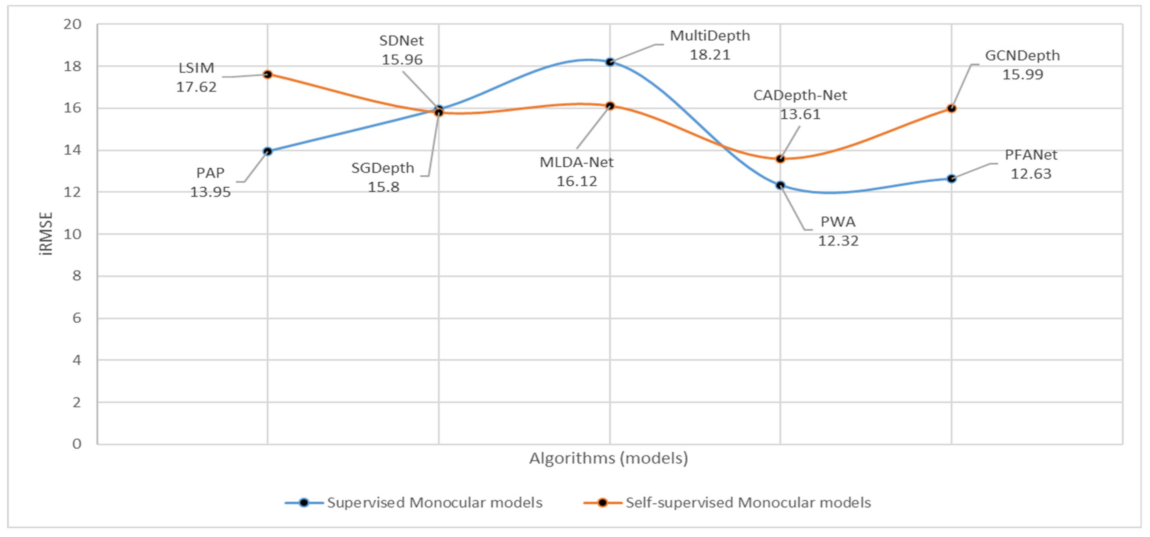
5.4. Experimental Comparison—Monocular Depth Estimation Models

Table 5. Comparison of supervised and self-supervised monocular depth estimation models on the online KITTI depth-prediction benchmark.

Sl. No.	Algorithms	Training Mode	SILog	sqErrRel	absErrRel	iRMSE	Runtime (s)
1	PAP [144]	Supervised	13.08	2.72	10.27	13.95	0.18
2	LSIM [140]	Self-supervised	17.92	6.88	14.04	17.62	0.08
3	SDNet [112]	Supervised	14.68	3.9	12.31	15.96	0.2
4	MultiDepth [111]	Supervised	16.05	3.89	13.82	18.21	0.01
5	SGDepth [142]	Self-supervised	15.3	5	13.29	15.8	0.1
6	MLDA-Net [145]	Self-supervised	14.42	3.41	11.67	16.12	0.2
7	PWA [109]	Supervised	11.45	2.3	9.05	12.32	0.06
8	PFANet [110]	Supervised	11.84	2.46	9.23	12.63	0.1
9	GCNDepth [141]	Self-supervised	15.54	4.26	12.75	15.99	0.05
10	CADepth-Net [143]	Self-supervised	13.34	3.33	10.67	13.61	0.08

depicts the year-wise comparison between the supervised and the self-supervised monocular depth estimation models on the KITTI depth prediction benchmark. The evaluation metrics used are SILog (Scale Invariant Logarithmic error), percentage of the relative squared error, percentage of the relative absolute error, and iRMSE (inverse-depth Root Mean Squared Error). The supervised methods show an increase in the metric values, specially from PAP [144] to SDNet [112] and then to MultiDepth [111], all in the year 2019. However, following that, the models PWA [109] and PFANet [110], in the year 2021, show a gradual decrease in the values and maintain a stability. The self-supervised methods, on the other hand, do have values exceeding those of the supervised models, indicating that development needs to be made with the recent rise in self-supervised approaches to reduce the gap to the supervised ones. To that effect, this is something which has been happening for the past few years. As can be observed, the progress made in self-supervised techniques is notable. The reduction in the values of the metrics from LSIM [140] to CADepth-Net [143], with small increments, implies the appreciable progress in the realm of self-supervised monocular depth estimation. Moreover, the computational runtimes of the self-supervised approaches are proving to be competitive when compared to those of the supervised ones. The feature extraction technique of multiple levels and the method of dual attention helps MLDA-Net [145] in attaining pixel-wise fine-quality depth maps with clarity of boundaries, which, in turn, provides appreciable values of metrics for the model. Similarly, the module of perception for the structures which enhances the structural perception of a scene and the module of emphasis which helps emphasize relevant information regarding the local details assist CADepth-Net [143] in obtaining accurate and sharp estimation of depth and significantly improved metric values. Figure 12 demonstrates a generalized view of the above scene, with respect to the iRMSE values for both model types. The supervised models show a decline and an almost flatline regarding the values after a steady rise. The self-supervised models, on the other hand, show a relatively smoother curve with a late rise, with some models having higher iRMSE values than the supervised models and with both model types falling within the same range of about a year.

6. Discussion—Future Research Prospects

For future work regarding depth estimation, certain areas can be worked on to enhance the process in terms of various parameters. Regarding both stereopsis and monocular depth prediction methods, the current processes have constraints in dealing with occlusions, regions having texture issues, disparities out of the training range, and the like. Research in the future can aim at establishing deep architectures of the robust kind that would be capable of dealing with such issues. Depth estimation has already been fused with processes like those of structured light, LiDAR, and others. Such conglomerations can be encouraged and improved to develop precise depth-sensing techniques. Future work can keep improving the unsupervised and the self-supervised learning techniques, which help reduce the need for labeled data. They also help in enhancing the generalization of the maps. However, sometimes training and re-training of the supervised methods on vast datasets transcends the generalizability characteristics of the self-supervised or the unsupervised methods in terms of the quality of depth maps produced.

Another prospect for further improvement in this field is real-time processing. Enhancement in speed without compromising efficiency is needed in real-world scenarios in autonomous vehicles and mobile robots. The existing architectures can be optimized or new ones with different neural dynamics can be developed, which helps in achieving the target. Furthermore, combining depth estimation with semantic segmentation and object recognition can lead to multi-tasking, which, if efficient, can further lead to a highly comprehensive scene understanding. To add to it, most depth estimation techniques are based on static structures, with just a few focusing on dynamic scenes. Future research work can concentrate on rapidly changing scenes to reflect real-world situations. Along with such merits, some disadvantages can always occur. Focusing on one parameter can force the compromise of another. However, careful analysis and proper understanding of the work with time can lead to a well-deserved balance between the parameters and even unprecedented improvements in the overall realm of depth estimation.

7. Conclusions

We have demonstrated a comprehensive review of contemporary progress in various stereo and monocular depth estimation techniques. While stereopsis requires relatively more resources and is more complicated to set up with the constraint on the length of the baseline, researchers have focused their target on the monocular depth technique, which requires the setting up of just a single RGB camera and is relatively inexpensive. The complexity of computation in stereo-matching techniques is higher than in monocular depth estimation methods. However, due to the refined quality of depth maps provided by stereopsis, stereo cameras continue to be competent enough concerning monocular depth cameras. The review provides evidence that machine learning, especially deep learning, is inevitable in current dense-depth estimation strategies. Deep learning finds its roots in the form of the various training methods followed in both the stereo and monocular depth estimation techniques, namely, supervised, unsupervised, and self-supervised. Supervised methods suffer from the issue of generalizability and the domain-shift problem. This is because the limited scope of the dataset does not capture all the characteristics of ill-posed regions in real life like poor illumination, texture, occlusions, and more. However, the problem with the unsupervised and the self-supervised method of learning is that they generally do not estimate absolute depth values and give only relative values of depth. Notwithstanding this, few processes train velocity or make use of IMU (Inertial Measurement Unit) sensors for predicting absolute values of depth. Eventually, due to the lack of availability of large ground-truth depth data, researchers have been trying to shift their target to unsupervised and self-supervised modes of training the frameworks. Various stereo vision and monocular methods are compared with each other in their respective category and the unsupervised and the self-supervised methods have been shown to perform incrementally better than their previous models and on par with the supervised models. Myriad research is in progress for estimating depth, which finds application not only in autonomous driving but also in biomedical sciences, robotics, underwater ROVs, various industrial mobile robots, and the like. We believe this review will be beneficial for researchers and students alike pursuing this field of research and for technologists delving into stereopsis and monocular depth techniques.

References

1. Tang, C.; Hou, C.; Song, Z. Depth recovery and refinement from a single image using defocus cues. J. Mod. Opt. 2015, 62, 441–448. [Google Scholar] [CrossRef]
2. Tsai, Y.-M.; Chang, Y.-L.; Chen, L.-G. Block-based vanishing line and vanishing point detection for 3D scene reconstruction. In Proceedings of the 2006 International Symposium on Intelligent Signal Processing and Communications, Yonago, Japan, 12–15 December 2006; pp. 586–589. [Google Scholar]
3. Zhang, R.; Tsai, P.-S.; Cryer, J.E.; Shah, M. Shape-from-shading: A survey. IEEE Trans. Pattern Anal. Mach. Intell. 1999, 21, 690–706. [Google Scholar] [CrossRef]
4. Bay, H.; Tuytelaars, T.; Van Gool, L. Surf: Speeded up robust features. Lect. Notes Comput. Sci. 2006, 3951, 404–417. [Google Scholar]
5. Bosch, A.; Zisserman, A.; Munoz, X. Image classification using random forests and ferns. In Proceedings of the 2007 IEEE 11th International Conference on Computer Vision, Rio De Janeiro, Brazil, 14–21 October 2007; pp. 1–8. [Google Scholar]
6. Lowe, D.G. Object recognition from local scale-invariant features. In Proceedings of the Seventh IEEE International Conference on Computer Vision, Kerkyra, Greece, 20–27 September 1999; pp. 1150–1157. [Google Scholar]
7. Lafferty, J.; McCallum, A.; Pereira, F.C. Conditional Random Fields: Probabilistic Models for Segmenting and Labeling Sequence Data. 2001. Available online: https://repository.upenn.edu/entities/publication/c9aea099-b5c8-4fdd-901c-15b6f889e4a7 (accessed on 28 June 2001).
8. Cross, G.R.; Jain, A.K. Markov random field texture models. IEEE Trans. Pattern Anal. Mach. Intell. 1983, PAMI-5, 25–39. [Google Scholar] [CrossRef] [PubMed]
9. Liu, B.; Gould, S.; Koller, D. Single image depth estimation from predicted semantic labels. In Proceedings of the 2010 IEEE Computer Society Conference on Computer Vision and Pattern Recognition, San Francisco, CA, USA, 13–18 June 2010; pp. 1253–1260. [Google Scholar]
10. Facil, J.M.; Ummenhofer, B.; Zhou, H.; Montesano, L.; Brox, T.; Civera, J. CAM-Convs: Camera-aware multi-scale convolutions for single-view depth. In Proceedings of the IEEE/CVF Conference on Computer Vision and Pattern Recognition, Long Beach, CA, USA, 15–20 June 2019; pp. 11826–11835. [Google Scholar]
11. Hao, S.; Zhou, Y.; Guo, Y. A brief survey on semantic segmentation with deep learning. Neurocomputing 2020, 406, 302–321. [Google Scholar] [CrossRef]
12. Lai, Z.; Lu, E.; Xie, W. Mast: A memory-augmented self-supervised tracker. In Proceedings of the IEEE/CVF Conference on Computer Vision and Pattern Recognition, Seattle, WA, USA, 13–19 June 2020; pp. 6479–6488. [Google Scholar]
13. Wang, K.; Peng, X.; Yang, J.; Lu, S.; Qiao, Y. Suppressing uncertainties for large-scale facial expression recognition. In Proceedings of the IEEE/CVF Conference on Computer Vision and Pattern Recognition, Seattle, WA, USA, 13–19 June 2020; pp. 6897–6906. [Google Scholar]
14. Zeng, N.; Zhang, H.; Song, B.; Liu, W.; Li, Y.; Dobaie, A.M. Facial expression recognition via learning deep sparse autoencoders. Neurocomputing 2018, 273, 643–649. [Google Scholar] [CrossRef]
15. Jin, L.; Wei, L.; Li, S. Gradient-based differential neural-solution to time-dependent nonlinear optimization. IEEE Trans. Autom. Control 2022, 68, 620–627. [Google Scholar] [CrossRef]
16. Gorban, A.N.; Mirkes, E.M.; Tyukin, I.Y. How deep should be the depth of convolutional neural networks: A backyard dog case study. Cogn. Comput. 2020, 12, 388–397. [Google Scholar] [CrossRef]
17. Liu, C.; Gu, J.; Kim, K.; Narasimhan, S.G.; Kautz, J. Neural rgb (r) d sensing: Depth and uncertainty from a video camera. In Proceedings of the IEEE/CVF Conference on Computer Vision and Pattern Recognition, Long Beach, CA, USA, 15–20 June 2019; pp. 10986–10995. [Google Scholar]
18. Ren, J.; Hussain, A.; Han, J.; Jia, X. Cognitive modelling and learning for multimedia mining and understanding. Cogn. Comput. 2019, 11, 761–762. [Google Scholar] [CrossRef]
19. Zbontar, J.; LeCun, Y. Stereo matching by training a convolutional neural network to compare image patches. J. Mach. Learn. Res. 2016, 17, 2287–2318. [Google Scholar]
20. Zhang, P.; Liu, J.; Wang, X.; Pu, T.; Fei, C.; Guo, Z. Stereoscopic video saliency detection based on spatiotemporal correlation and depth confidence optimization. Neurocomputing 2020, 377, 256–268. [Google Scholar] [CrossRef]
21. Zhang, Z. A flexible new technique for camera calibration. IEEE Trans. Pattern Anal. Mach. Intell. 2000, 22, 1330–1334. [Google Scholar] [CrossRef]
22. Liu, F.; Zhou, S.; Wang, Y.; Hou, G.; Sun, Z.; Tan, T. Binocular light-field: Imaging theory and occlusion-robust depth perception application. IEEE Trans. Image Process. 2019, 29, 1628–1640. [Google Scholar] [CrossRef] [PubMed]
23. Mur-Artal, R.; Montiel, J.M.M.; Tardos, J.D. ORB-SLAM: A versatile and accurate monocular SLAM system. IEEE Trans. Robot. 2015, 31, 1147–1163. [Google Scholar] [CrossRef]
24. Bhoi, A. Monocular depth estimation: A survey. arXiv 2019, arXiv:1901.09402. [Google Scholar]
25. Laga, H. A survey on deep learning architectures for image-based depth reconstruction. arXiv 2019, arXiv:1906.06113. [Google Scholar]
26. Scharstein, D.; Szeliski, R. A taxonomy and evaluation of dense two-frame stereo correspondence algorithms. Int. J. Comput. Vis. 2002, 47, 7–42. [Google Scholar] [CrossRef]
27. Scharstein, D.; Szeliski, R. High-accuracy stereo depth maps using structured light. In Proceedings of the 2003 IEEE Computer Society Conference on Computer Vision and Pattern Recognition, Madison, WI, USA, 18–20 June 2003; p. I. [Google Scholar]
28. Hirschmuller, H.; Scharstein, D. Evaluation of cost functions for stereo matching. In Proceedings of the 2007 IEEE Conference on Computer Vision and Pattern Recognition, Minneapolis, MN, USA, 17–22 June 2007; pp. 1–8. [Google Scholar]
29. Geiger, A.; Lenz, P.; Urtasun, R. Are we ready for autonomous driving? The kitti vision benchmark suite. In Proceedings of the 2012 IEEE Conference on Computer Vision and Pattern Recognition, Providence, RI, USA, 16–21 June 2012; pp. 3354–3361. [Google Scholar]
30. Scharstein, D.; Hirschmüller, H.; Kitajima, Y.; Krathwohl, G.; Nešić, N.; Wang, X.; Westling, P. High-resolution stereo datasets with subpixel-accurate ground truth. In Proceedings of the Pattern Recognition: 36th German Conference, GCPR 2014, Münster, Germany, 2–5 September 2014; Proceedings 36. pp. 31–42. [Google Scholar]
31. LeCun, Y.; Bengio, Y.; Hinton, G. Deep learning. Nature 2015, 521, 436–444. [Google Scholar] [CrossRef]
32. Geiger, A.; Lenz, P.; Stiller, C.; Urtasun, R. Vision meets robotics: The kitti dataset. Int. J. Robot. Res. 2013, 32, 1231–1237. [Google Scholar] [CrossRef]
33. Mayer, N.; Ilg, E.; Hausser, P.; Fischer, P.; Cremers, D.; Dosovitskiy, A.; Brox, T. A large dataset to train convolutional networks for disparity, optical flow, and scene flow estimation. In Proceedings of the IEEE Conference on Computer Vision and Pattern Recognition, Las Vegas, NV, USA, 27–30 June 2016; pp. 4040–4048. [Google Scholar]
34. Mayer, N.; Ilg, E.; Fischer, P.; Hazirbas, C.; Cremers, D.; Dosovitskiy, A.; Brox, T. What makes good synthetic training data for learning disparity and optical flow estimation? Int. J. Comput. Vis. 2018, 126, 942–960. [Google Scholar] [CrossRef]
35. Silberman, N.; Hoiem, D.; Kohli, P.; Fergus, R. Indoor segmentation and support inference from rgbd images. In Proceedings of the Computer Vision–ECCV 2012: 12th European Conference on Computer Vision, Florence, Italy, 7–13 October 2012; Proceedings, Part V 12. pp. 746–760. [Google Scholar]
36. Jensen, R.; Dahl, A.; Vogiatzis, G.; Tola, E.; Aanæs, H. Large scale multi-view stereopsis evaluation. In Proceedings of the IEEE Conference on Computer Vision and Pattern Recognition, Columbus, OH, USA, 23–28 June 2014; pp. 406–413. [Google Scholar]
37. Schops, T.; Schonberger, J.L.; Galliani, S.; Sattler, T.; Schindler, K.; Pollefeys, M.; Geiger, A. A multi-view stereo benchmark with high-resolution images and multi-camera videos. In Proceedings of the IEEE Conference on Computer Vision and Pattern Recognition, Honolulu, HI, USA, 21–26 July 2017; pp. 3260–3269. [Google Scholar]
38. Pang, J.; Sun, W.; Ren, J.S.; Yang, C.; Yan, Q. Cascade residual learning: A two-stage convolutional neural network for stereo matching. In Proceedings of the IEEE International Conference on Computer Vision Workshops, Venice, Italy, 22–29 October 2017; pp. 887–895. [Google Scholar]
39. Jia, Y.; Shelhamer, E.; Donahue, J.; Karayev, S.; Long, J.; Girshick, R.; Guadarrama, S.; Darrell, T. Caffe: Convolutional architecture for fast feature embedding. In Proceedings of the 22nd ACM International Conference on Multimedia, Orlando, FL, USA, 3–7 November 2014; pp. 675–678. [Google Scholar]
40. Chang, J.-R.; Chen, Y.-S. Pyramid stereo matching network. In Proceedings of the IEEE Conference on Computer Vision and Pattern Recognition, Salt Lake City, UT, USA, 18–22 June 2018; pp. 5410–5418. [Google Scholar]
41. Khamis, S.; Fanello, S.; Rhemann, C.; Kowdle, A.; Valentin, J.; Izadi, S. Stereonet: Guided hierarchical refinement for real-time edge-aware depth prediction. In Proceedings of the European Conference on Computer Vision (ECCV), Munich, Germany, 8–14 September 2018; pp. 573–590. [Google Scholar]
42. Hinton, G.; Srivastava, N.; Swersky, K. Neural networks for machine learning lecture 6a overview of mini-batch gradient descent. Cited 2012, 14, 2. [Google Scholar]
43. Song, X.; Zhao, X.; Hu, H.; Fang, L. Edgestereo: A context integrated residual pyramid network for stereo matching. In Proceedings of the Computer Vision–ACCV 2018: 14th Asian Conference on Computer Vision, Perth, Australia, 2–6 December 2018; Revised Selected Papers Part V 14. pp. 20–35. [Google Scholar]
44. Liu, Y.; Cheng, M.-M.; Hu, X.; Wang, K.; Bai, X. Richer convolutional features for edge detection. In Proceedings of the IEEE Conference on Computer Vision and Pattern Recognition, Honolulu, HI, USA, 21–26 July 2017; pp. 3000–3009. [Google Scholar]
45. Arbelaez, P.; Maire, M.; Fowlkes, C.; Malik, J. Contour detection and hierarchical image segmentation. IEEE Trans. Pattern Anal. Mach. Intell. 2010, 33, 898–916. [Google Scholar] [CrossRef] [PubMed]
46. Liu, Y.; Lew, M.S. Learning relaxed deep supervision for better edge detection. In Proceedings of the IEEE Conference on Computer Vision and Pattern Recognition, Las Vegas, NV, USA, 27–30 June 2016; pp. 231–240. [Google Scholar]
47. Mottaghi, R.; Chen, X.; Liu, X.; Cho, N.-G.; Lee, S.-W.; Fidler, S.; Urtasun, R.; Yuille, A. The role of context for object detection and semantic segmentation in the wild. In Proceedings of the IEEE Conference on Computer Vision and Pattern Recognition, Columbus, OH, USA, 23–28 June 2014; pp. 891–898. [Google Scholar]
48. Kingma, D.P.; Ba, J. Adam: A method for stochastic optimization. arXiv 2014, arXiv:1412.6980. [Google Scholar]
49. Wang, Y.; Lai, Z.; Huang, G.; Wang, B.H.; Van Der Maaten, L.; Campbell, M.; Weinberger, K.Q. Anytime stereo image depth estimation on mobile devices. In Proceedings of the 2019 International Conference on Robotics and Automation (ICRA), Montreal, QC, Canada, 20–24 May 2019; pp. 5893–5900. [Google Scholar]
50. Yang, G.; Manela, J.; Happold, M.; Ramanan, D. Hierarchical deep stereo matching on high-resolution images. In Proceedings of the IEEE/CVF Conference on Computer Vision and Pattern Recognition, Long Beach, CA, USA, 15–20 June 2019; pp. 5515–5524. [Google Scholar]
51. Menze, M.; Geiger, A. Object scene flow for autonomous vehicles. In Proceedings of the IEEE Conference on Computer Vision and Pattern Recognition, Boston, MA, USA, 7–12 June 2015; pp. 3061–3070. [Google Scholar]
52. Liang, Z.; Guo, Y.; Feng, Y.; Chen, W.; Qiao, L.; Zhou, L.; Zhang, J.; Liu, H. Stereo matching using multi-level cost volume and multi-scale feature constancy. IEEE Trans. Pattern Anal. Mach. Intell. 2019, 43, 300–315. [Google Scholar] [CrossRef] [PubMed]
53. Xu, Q.; Tao, W. Pvsnet: Pixelwise visibility-aware multi-view stereo network. arXiv 2020, arXiv:2007.07714. [Google Scholar]
54. Ji, M.; Gall, J.; Zheng, H.; Liu, Y.; Fang, L. Surfacenet: An end-to-end 3d neural network for multiview stereopsis. In Proceedings of the IEEE International Conference on Computer Vision, Venice, Italy, 22–29 October 2017; pp. 2307–2315. [Google Scholar]
55. Yao, Y.; Luo, Z.; Li, S.; Fang, T.; Quan, L. Mvsnet: Depth inference for unstructured multi-view stereo. In Proceedings of the European Conference on Computer vision (ECCV), Munich, Germany, 8–14 September 2018; pp. 767–783. [Google Scholar]
56. Aanæs, H.; Jensen, R.R.; Vogiatzis, G.; Tola, E.; Dahl, A.B. Large-scale data for multiple-view stereopsis. Int. J. Comput. Vis. 2016, 120, 153–168. [Google Scholar] [CrossRef]
57. Kazhdan, M.; Hoppe, H. Screened poisson surface reconstruction. ACM Trans. Graph. (ToG) 2013, 32, 1–13. [Google Scholar] [CrossRef]
58. Paszke, A.; Gross, S.; Massa, F.; Lerer, A.; Bradbury, J.; Chanan, G.; Killeen, T.; Lin, Z.; Gimelshein, N.; Antiga, L. Pytorch: An imperative style, high-performance deep learning library. arXiv 2019, arXiv:1912.01703. [Google Scholar]
59. Tankovich, V.; Hane, C.; Zhang, Y.; Kowdle, A.; Fanello, S.; Bouaziz, S. Hitnet: Hierarchical iterative tile refinement network for real-time stereo matching. In Proceedings of the IEEE/CVF Conference on Computer Vision and Pattern Recognition, Nashville, TN, USA, 20–25 June 2021; pp. 14362–14372. [Google Scholar]
60. Ronneberger, O.; Fischer, P.; Brox, T. U-net: Convolutional networks for biomedical image segmentation. In Proceedings of the Medical Image Computing and Computer-Assisted Intervention–MICCAI 2015: 18th International Conference, Munich, Germany, 5–9 October 2015; Proceedings, Part III 18. pp. 234–241. [Google Scholar]
61. Lipson, L.; Teed, Z.; Deng, J. Raft-stereo: Multilevel recurrent field transforms for stereo matching. In Proceedings of the 2021 International Conference on 3D Vision (3DV), London, UK, 1–3 December 2021; pp. 218–227. [Google Scholar]
62. Teed, Z.; Deng, J. Raft: Recurrent all-pairs field transforms for optical flow. In Proceedings of the Computer Vision–ECCV 2020: 16th European Conference, Glasgow, UK, 23–28 August 2020; Proceedings, Part II 16. pp. 402–419. [Google Scholar]
63. Paszke, A.; Gross, S.; Chintala, S.; Chanan, G.; Yang, E.; DeVito, Z.; Lin, Z.; Desmaison, A.; Antiga, L.; Lerer, A. Automatic Differentiation in Pytorch, BibSonomy, Long Beach, California, USA. Available online: https://openreview.net/forum?id=BJJsrmfCZ (accessed on 28 October 2017).
64. Loshchilov, I.; Hutter, F. Decoupled weight decay regularization. arXiv 2017, arXiv:1711.05101. [Google Scholar]
65. Zeng, L.; Tian, X. CRAR: Accelerating Stereo Matching with Cascaded Residual Regression and Adaptive Refinement. ACM Trans. Multimed. Comput. Commun. Appl. (TOMM) 2022, 18, 1–19. [Google Scholar] [CrossRef]
66. Yin, Z.; Darrell, T.; Yu, F. Hierarchical discrete distribution decomposition for match density estimation. In Proceedings of the IEEE/CVF Conference on Computer Vision and Pattern Recognition, Long Beach, CA, USA, 15–20 June 2019; pp. 6044–6053. [Google Scholar]
67. Zhang, F.; Prisacariu, V.; Yang, R.; Torr, P.H. Ga-net: Guided aggregation net for end-to-end stereo matching. In Proceedings of the IEEE/CVF Conference on Computer Vision and Pattern Recognition, Long Beach, CA, USA, 15–20 June 2019; pp. 185–194. [Google Scholar]
68. Xu, G.; Cheng, J.; Guo, P.; Yang, X. Attention concatenation volume for accurate and efficient stereo matching. In Proceedings of the IEEE/CVF Conference on Computer Vision and Pattern Recognition, New Orleans, LA, USA, 18–24 June 2022; pp. 12981–12990. [Google Scholar]
69. Jiang, H.; Xu, R.; Jiang, W. An Improved RaftStereo Trained with A Mixed Dataset for the Robust Vision Challenge 2022. arXiv 2022, arXiv:2210.12785. [Google Scholar]
70. Shen, Z.; Dai, Y.; Song, X.; Rao, Z.; Zhou, D.; Zhang, L. Pcw-net: Pyramid combination and warping cost volume for stereo matching. In Proceedings of the Computer Vision–ECCV 2022: 17th European Conference, Tel Aviv, Israel, 23–27 October 2022; Proceedings, Part XXXI. pp. 280–297. [Google Scholar]
71. Guo, X.; Yang, K.; Yang, W.; Wang, X.; Li, H. Group-wise correlation stereo network. In Proceedings of the IEEE/CVF Conference on Computer Vision and Pattern Recognition, Long Beach, CA, USA, 15–20 June 2019; pp. 3273–3282. [Google Scholar]
72. Xu, G.; Zhou, H.; Yang, X. CGI-Stereo: Accurate and Real-Time Stereo Matching via Context and Geometry Interaction. arXiv 2023, arXiv:2301.02789. [Google Scholar]
73. Khot, T.; Agrawal, S.; Tulsiani, S.; Mertz, C.; Lucey, S.; Hebert, M. Learning unsupervised multi-view stereopsis via robust photometric consistency. arXiv 2019, arXiv:1905.02706. [Google Scholar]
74. Abadi, M.; Barham, P.; Chen, J.; Chen, Z.; Davis, A.; Dean, J.; Devin, M.; Ghemawat, S.; Irving, G.; Isard, M. Tensorflow: A system for large-scale machine learning. In Proceedings of the OSDI, Savannah, GA, USA, 2–4 November 2016; pp. 265–283. [Google Scholar]
75. Dai, Y.; Zhu, Z.; Rao, Z.; Li, B. Mvs2: Deep unsupervised multi-view stereo with multi-view symmetry. In Proceedings of the 2019 International Conference on 3D Vision (3DV), Quebec City, QC, Canada, 16–19 September 2019; pp. 1–8. [Google Scholar]
76. Pilzer, A.; Lathuilière, S.; Xu, D.; Puscas, M.M.; Ricci, E.; Sebe, N. Progressive fusion for unsupervised binocular depth estimation using cycled networks. IEEE Trans. Pattern Anal. Mach. Intell. 2019, 42, 2380–2395. [Google Scholar] [CrossRef] [PubMed]
77. Mao, X.; Li, Q.; Xie, H.; Lau, R.Y.; Wang, Z.; Paul Smolley, S. Least squares generative adversarial networks. In Proceedings of the IEEE International Conference on Computer Vision, Venice, Italy, 22–29 October 2017; pp. 2794–2802. [Google Scholar]
78. Huang, B.; Yi, H.; Huang, C.; He, Y.; Liu, J.; Liu, X. M3VSNet: Unsupervised multi-metric multi-view stereo network. In Proceedings of the 2021 IEEE International Conference on Image Processing (ICIP), Anchorage, AK, USA, 19–22 September 2021; pp. 3163–3167. [Google Scholar]
79. Qi, S.; Sang, X.; Yan, B.; Wang, P.; Chen, D.; Wang, H.; Ye, X. Unsupervised multi-view stereo network based on multi-stage depth estimation. Image Vis. Comput. 2022, 122, 104449. [Google Scholar] [CrossRef]
80. Sun, D.; Yang, X.; Liu, M.-Y.; Kautz, J. Pwc-net: Cnns for optical flow using pyramid, warping, and cost volume. In Proceedings of the IEEE Conference on Computer Vision and Pattern Recognition, Salt Lake City, UT, USA, 18–22 June 2018; pp. 8934–8943. [Google Scholar]
81. Xu, H.; Zhou, Z.; Wang, Y.; Kang, W.; Sun, B.; Li, H.; Qiao, Y. Digging into uncertainty in self-supervised multi-view stereo. In Proceedings of the IEEE/CVF International Conference on Computer Vision, Montreal, BC, Canada, 11–17 October 2021; pp. 6078–6087. [Google Scholar]
82. Loshchilov, I.; Hutter, F. Sgdr: Stochastic gradient descent with warm restarts. arXiv 2016, arXiv:1608.03983. [Google Scholar]
83. Huang, B.; Zheng, J.-Q.; Giannarou, S.; Elson, D.S. H-net: Unsupervised attention-based stereo depth estimation leveraging epipolar geometry. In Proceedings of the IEEE/CVF Conference on Computer Vision and Pattern Recognition, New Orleans, LA, USA, 18–24 June 2022; pp. 4460–4467. [Google Scholar]
84. Gan, W.; Wong, P.K.; Yu, G.; Zhao, R.; Vong, C.M. Light-weight network for real-time adaptive stereo depth estimation. Neurocomputing 2021, 441, 118–127. [Google Scholar] [CrossRef]
85. Cheng, X.; Wang, P.; Yang, R. Learning depth with convolutional spatial propagation network. IEEE Trans. Pattern Anal. Mach. Intell. 2019, 42, 2361–2379. [Google Scholar] [CrossRef]
86. Yang, J.; Alvarez, J.M.; Liu, M. Self-supervised learning of depth inference for multi-view stereo. In Proceedings of the IEEE/CVF Conference on Computer Vision and Pattern Recognition, Nashville, TN, USA, 20–25 June 2021; pp. 7526–7534. [Google Scholar]
87. Yang, J.; Mao, W.; Alvarez, J.M.; Liu, M. Cost volume pyramid based depth inference for multi-view stereo. In Proceedings of the IEEE/CVF Conference on Computer Vision and Pattern Recognition, Seattle, WA, USA, 13–19 June 2020; pp. 4877–4886. [Google Scholar]
88. Johnson, J.; Alahi, A.; Fei-Fei, L. Perceptual losses for real-time style transfer and super-resolution. In Proceedings of the Computer Vision–ECCV 2016: 14th European Conference, Amsterdam, The Netherlands, 11–14 October 2016; Proceedings, Part II 14. pp. 694–711. [Google Scholar]
89. Wang, C.; Bai, X.; Wang, X.; Liu, X.; Zhou, J.; Wu, X.; Li, H.; Tao, D. Self-supervised multiscale adversarial regression network for stereo disparity estimation. IEEE Trans. Cybern. 2020, 51, 4770–4783. [Google Scholar] [CrossRef]
90. Huang, B.; Zheng, J.-Q.; Nguyen, A.; Tuch, D.; Vyas, K.; Giannarou, S.; Elson, D.S. Self-supervised generative adversarial network for depth estimation in laparoscopic images. In Proceedings of the Medical Image Computing and Computer Assisted Intervention–MICCAI 2021: 24th International Conference, Strasbourg, France, 27 September–1 October 2021; Proceedings, Part IV 24. pp. 227–237. [Google Scholar]
91. Zhong, Y.; Dai, Y.; Li, H. Self-supervised learning for stereo matching with self-improving ability. arXiv 2017, arXiv:1709.00930. [Google Scholar]
92. Wang, H.; Fan, R.; Cai, P.; Liu, M. PVStereo: Pyramid voting module for end-to-end self-supervised stereo matching. IEEE Robot. Autom. Lett. 2021, 6, 4353–4360. [Google Scholar] [CrossRef]
93. Li, J.; Wang, P.; Xiong, P.; Cai, T.; Yan, Z.; Yang, L.; Liu, J.; Fan, H.; Liu, S. Practical stereo matching via cascaded recurrent network with adaptive correlation. In Proceedings of the IEEE/CVF Conference on Computer Vision and Pattern Recognition, New Orleans, LA, USA, 18–24 June 2022; pp. 16263–16272. [Google Scholar]
94. Zhao, H.; Zhou, H.; Zhang, Y.; Zhao, Y.; Yang, Y.; Ouyang, T. EAI-Stereo: Error Aware Iterative Network for Stereo Matching. In Proceedings of the Asian Conference on Computer Vision, Macao, China, 4–8 December 2022; pp. 315–332. [Google Scholar]
95. Fu, H.; Gong, M.; Wang, C.; Batmanghelich, K.; Tao, D. Deep ordinal regression network for monocular depth estimation. In Proceedings of the IEEE Conference on Computer Vision and Pattern Recognition, Salt Lake City, UT, USA, 18–22 June 2018; pp. 2002–2011. [Google Scholar]
96. Chen, Y.; Zhao, H.; Hu, Z.; Peng, J. Attention-based context aggregation network for monocular depth estimation. Int. J. Mach. Learn. Cybern. 2021, 12, 1583–1596. [Google Scholar] [CrossRef]
97. Vaswani, A.; Shazeer, N.; Parmar, N.; Uszkoreit, J.; Jones, L.; Gomez, A.N.; Kaiser, Ł.; Polosukhin, I. Attention is all you need. arXiv 2017, arXiv:1706.03762. [Google Scholar]
98. Wang, X.; Girshick, R.; Gupta, A.; He, K. Non-local neural networks. In Proceedings of the IEEE Conference on Computer Vision and Pattern Recognition, Salt Lake City, UT, USA, 18–22 June 2018; pp. 7794–7803. [Google Scholar]
99. Liu, W.; Rabinovich, A.; Berg, A.C. Parsenet: Looking wider to see better. arXiv 2015, arXiv:1506.04579. [Google Scholar]
100. Chen, L.-C.; Papandreou, G.; Schroff, F.; Adam, H. Rethinking atrous convolution for semantic image segmentation. arXiv 2017, arXiv:1706.0558. [Google Scholar]
101. Cao, Y.; Zhao, T.; Xian, K.; Shen, C.; Cao, Z.; Xu, S. Monocular depth estimation with augmented ordinal depth relationships. IEEE Trans. Image Process. 2019, 30, 2674–2682. [Google Scholar]
102. Chang, J.; Wetzstein, G. Deep optics for monocular depth estimation and 3d object detection. In Proceedings of the IEEE/CVF International Conference on Computer Vision, Seoul, Republic of Korea, 27 October–2 November 2019; pp. 10193–10202. [Google Scholar]
103. Yin, W.; Liu, Y.; Shen, C.; Yan, Y. Enforcing geometric constraints of virtual normal for depth prediction. In Proceedings of the IEEE/CVF International Conference on Computer Vision, Seoul, Republic of Korea, 27 October–2 November 2019; pp. 5684–5693. [Google Scholar]
104. Cao, Y.; Wu, Z.; Shen, C. Estimating depth from monocular images as classification using deep fully convolutional residual networks. IEEE Trans. Circuits Syst. Video Technol. 2017, 28, 3174–3182. [Google Scholar] [CrossRef]
105. Xie, S.; Girshick, R.; Dollár, P.; Tu, Z.; He, K. Aggregated residual transformations for deep neural networks. In Proceedings of the IEEE Conference on Computer Vision and Pattern Recognition, Honolulu, HI, USA, 21–26 July 2017; pp. 1492–1500. [Google Scholar]
106. Deng, J.; Dong, W.; Socher, R.; Li, L.-J.; Li, K.; Fei-Fei, L. Imagenet: A large-scale hierarchical image database. In Proceedings of the 2009 IEEE Conference on Computer Vision and Pattern Recognition, Miami, FL, USA, 20–25 June 2009; pp. 248–255. [Google Scholar]
107. Lee, J.H.; Han, M.-K.; Ko, D.W.; Suh, I.H. From big to small: Multi-scale local planar guidance for monocular depth estimation. arXiv 2019, arXiv:1907.10326. [Google Scholar]
108. Eigen, D.; Puhrsch, C.; Fergus, R. Depth map prediction from a single image using a multi-scale deep network. arXiv 2014, arXiv:1406.2283. [Google Scholar]
109. Lee, S.; Lee, J.; Kim, B.; Yi, E.; Kim, J. Patch-wise attention network for monocular depth estimation. In Proceedings of the AAAI Conference on Artificial Intelligence, Virtual, 2–9 February 2021; pp. 1873–1881. [Google Scholar]
110. Xu, Y.; Peng, C.; Li, M.; Li, Y.; Du, S. Pyramid feature attention network for monocular depth prediction. In Proceedings of the 2021 IEEE International Conference on Multimedia and Expo (ICME), Shenzhen, China, 5–9 July 2021; pp. 1–6. [Google Scholar]
111. Liebel, L.; Körner, M. Multidepth: Single-image depth estimation via multi-task regression and classification. In Proceedings of the 2019 IEEE Intelligent Transportation Systems Conference (ITSC), Auckland, New Zealand, 27–30 October 2019; pp. 1440–1447. [Google Scholar]
112. Ochs, M.; Kretz, A.; Mester, R. Sdnet: Semantically guided depth estimation network. In Proceedings of the Pattern Recognition: 41st DAGM German Conference, DAGM GCPR 2019, Dortmund, Germany, 10–13 September 2019; Proceedings 41. pp. 288–302. [Google Scholar]
113. Lei, Z.; Wang, Y.; Li, Z.; Yang, J. Attention based multilayer feature fusion convolutional neural network for unsupervised monocular depth estimation. Neurocomputing 2021, 423, 343–352. [Google Scholar] [CrossRef]
114. Ji, Z.-y.; Song, X.-j.; Song, H.-b.; Yang, H.; Guo, X.-x. RDRF-Net: A pyramid architecture network with residual-based dynamic receptive fields for unsupervised depth estimation. Neurocomputing 2021, 457, 1–12. [Google Scholar] [CrossRef]
115. Poggi, M.; Aleotti, F.; Tosi, F.; Mattoccia, S. Towards real-time unsupervised monocular depth estimation on cpu. In Proceedings of the 2018 IEEE/RSJ International Conference on Intelligent Robots and Systems (IROS), Madrid, Spain, 1–5 October 2018; pp. 5848–5854. [Google Scholar]
116. Chen, P.-Y.; Liu, A.H.; Liu, Y.-C.; Wang, Y.-C.F. Towards scene understanding: Unsupervised monocular depth estimation with semantic-aware representation. In Proceedings of the IEEE/CVF Conference on Computer Vision and Pattern Recognition, Long Beach, CA, USA, 15–20 June 2019; pp. 2624–2632. [Google Scholar]
117. Godard, C.; Mac Aodha, O.; Brostow, G.J. Unsupervised monocular depth estimation with left-right consistency. In Proceedings of the IEEE Conference on Computer Vision and Pattern Recognition, Honolulu, HI, USA, 21–26 July 2017; pp. 270–279. [Google Scholar]
118. Repala, V.K.; Dubey, S.R. Dual cnn models for unsupervised monocular depth estimation. In Proceedings of the Pattern Recognition and Machine Intelligence: 8th International Conference, PReMI 2019, Tezpur, India, 17–20 December 2019; Proceedings, Part I. pp. 209–217. [Google Scholar]
119. Ling, C.; Zhang, X.; Chen, H. Unsupervised monocular depth estimation using attention and multi-warp reconstruction. IEEE Trans. Multimed. 2021, 24, 2938–2949. [Google Scholar] [CrossRef]
120. Wang, H.; Sun, Y.; Wu, Q.J.; Lu, X.; Wang, X.; Zhang, Z. Self-supervised monocular depth estimation with direct methods. Neurocomputing 2021, 421, 340–348. [Google Scholar] [CrossRef]
121. Bartoccioni, F.; Zablocki, É.; Pérez, P.; Cord, M.; Alahari, K. LiDARTouch: Monocular metric depth estimation with a few-beam LiDAR. Comput. Vis. Image Underst. 2023, 227, 103601. [Google Scholar] [CrossRef]
122. Zhou, T.; Brown, M.; Snavely, N.; Lowe, D.G. Unsupervised learning of depth and ego-motion from video. In Proceedings of the IEEE Conference on Computer Vision and Pattern Recognition, Honolulu, HI, USA, 21–26 July 2017; pp. 1851–1858. [Google Scholar]
123. Godard, C.; Mac Aodha, O.; Firman, M.; Brostow, G.J. Digging into self-supervised monocular depth estimation. In Proceedings of the IEEE/CVF International Conference on Computer Vision, Seoul, Republic of Korea, 27 October–2 November 2019; pp. 3828–3838. [Google Scholar]
124. Lu, K.; Zeng, C.; Zeng, Y. Self-supervised learning of monocular depth using quantized networks. Neurocomputing 2022, 488, 634–646. [Google Scholar] [CrossRef]
125. Kerr, A.; Merrill, D.; Demouth, J.; Tran, J.; Farooqui, N.; Tavenrath, M.; Schuster, V.; Gornish, E.; Zheng, J.; Sathe, B. CUTLASS: CUDA Template Library for Dense Linear Algebra at all levels and scales. Available online: https://on-demand.gputechconf.com/gtc/2018/presentation/s8854-cutlass-software-primitives-for-dense-linear-algebra-at-all-levels-and-scales-within-cuda.pdf (accessed on 29 March 2018).
126. Choi, J.; Jung, D.; Lee, Y.; Kim, D.; Manocha, D.; Lee, D. SelfTune: Metrically Scaled Monocular Depth Estimation through Self-Supervised Learning. In Proceedings of the 2022 International Conference on Robotics and Automation (ICRA), Philadelphia, PA, USA, 23–27 May 2022; pp. 6511–6518. [Google Scholar]
127. Ranftl, R.; Lasinger, K.; Hafner, D.; Schindler, K.; Koltun, V. Towards robust monocular depth estimation: Mixing datasets for zero-shot cross-dataset transfer. IEEE Trans. Pattern Anal. Mach. Intell. 2020, 44, 1623–1637. [Google Scholar] [CrossRef] [PubMed]
128. Yin, W.; Zhang, J.; Wang, O.; Niklaus, S.; Mai, L.; Chen, S.; Shen, C. Learning to recover 3d scene shape from a single image. In Proceedings of the IEEE/CVF Conference on Computer Vision and Pattern Recognition, Nashville, TN, USA, 20–25 June 2021; pp. 204–213. [Google Scholar]
129. Qin, T.; Li, P.; Shen, S. Vins-mono: A robust and versatile monocular visual-inertial state estimator. IEEE Trans. Robot. 2018, 34, 1004–1020. [Google Scholar] [CrossRef]
130. Li, Z.; Snavely, N. Megadepth: Learning single-view depth prediction from internet photos. In Proceedings of the IEEE Conference on Computer Vision and Pattern Recognition, Salt Lake City, UT, USA, 18–22 June 2018; pp. 2041–2050. [Google Scholar]
131. Yue, M.; Fu, G.; Wu, M.; Zhang, X.; Gu, H. Self-supervised monocular depth estimation in dynamic scenes with moving instance loss. Eng. Appl. Artif. Intell. 2022, 112, 104862. [Google Scholar] [CrossRef]
132. Yang, X.; Zhang, X.; Wang, N.; Xin, G.; Hu, W. Underwater self-supervised depth estimation. Neurocomputing 2022, 514, 362–373. [Google Scholar] [CrossRef]
133. Ilg, E.; Mayer, N.; Saikia, T.; Keuper, M.; Dosovitskiy, A.; Brox, T. Flownet 2.0: Evolution of optical flow estimation with deep networks. In Proceedings of the IEEE Conference on Computer Vision and Pattern Recognition, Honolulu, HI, USA, 21–26 July 2017; pp. 2462–2470. [Google Scholar]
134. Hwang, S.-J.; Park, S.-J.; Baek, J.-H.; Kim, B. Self-supervised monocular depth estimation using hybrid transformer encoder. IEEE Sens. J. 2022, 22, 18762–18770. [Google Scholar] [CrossRef]
135. Watson, J.; Mac Aodha, O.; Prisacariu, V.; Brostow, G.; Firman, M. The temporal opportunist: Self-supervised multi-frame monocular depth. In Proceedings of the IEEE/CVF Conference on Computer Vision and Pattern Recognition, Nashville, TN, USA, 20–25 June 2021; pp. 1164–1174. [Google Scholar]
136. Chawla, H.; Jeeveswaran, K.; Arani, E.; Zonooz, B. Image Masking for Robust Self-Supervised Monocular Depth Estimation. arXiv 2022, arXiv:2210.02357. [Google Scholar]
137. Varma, A.; Chawla, H.; Zonooz, B.; Arani, E. Transformers in self-supervised monocular depth estimation with unknown camera intrinsics. arXiv 2022, arXiv:2202.03131. [Google Scholar]
138. Cai, H.; Yin, F.; Singhal, T.; Pendyam, S.; Noorzad, P.; Zhu, Y.; Nguyen, K.; Matai, J.; Ramaswamy, B.; Mayer, F. Real-Time and Accurate Self-Supervised Monocular Depth Estimation on Mobile Device. In Proceedings of the NeurIPS 2021 Competitions and Demonstrations Track, Online, 6–14 December 2021; pp. 308–313. [Google Scholar]
139. Cai, H.; Matai, J.; Borse, S.; Zhang, Y.; Ansari, A.; Porikli, F. X-distill: Improving self-supervised monocular depth via cross-task distillation. arXiv 2021, arXiv:2110.12516. [Google Scholar]
140. Goldman, M.; Hassner, T.; Avidan, S. Learn stereo, infer mono: Siamese networks for self-supervised, monocular, depth estimation. In Proceedings of the IEEE/CVF Conference on Computer Vision and Pattern Recognition Workshops, Long Beach, CA, USA, 16–17 June 2019. [Google Scholar]
141. Masoumian, A.; Rashwan, H.A.; Abdulwahab, S.; Cristiano, J.; Asif, M.S.; Puig, D. GCNDepth: Self-supervised monocular depth estimation based on graph convolutional network. Neurocomputing 2023, 517, 81–92. [Google Scholar] [CrossRef]
142. Klingner, M.; Termöhlen, J.-A.; Mikolajczyk, J.; Fingscheidt, T. Self-supervised monocular depth estimation: Solving the dynamic object problem by semantic guidance. In Proceedings of the Computer Vision–ECCV 2020: 16th European Conference, Glasgow, UK, 23–28 August 2020; Proceedings, Part XX 16. pp. 582–600. [Google Scholar]
143. Yan, J.; Zhao, H.; Bu, P.; Jin, Y. Channel-wise attention-based network for self-supervised monocular depth estimation. In Proceedings of the 2021 International Conference on 3D Vision (3DV), London, UK, 1–3 December 2021; pp. 464–473. [Google Scholar]
144. Zhang, Z.; Cui, Z.; Xu, C.; Yan, Y.; Sebe, N.; Yang, J. Pattern-affinitive propagation across depth, surface normal and semantic segmentation. In Proceedings of the IEEE/CVF Conference on Computer Vision and Pattern Recognition, Long Beach, CA, USA, 15–20 June 2019; pp. 4106–4115. [Google Scholar]
145. Song, X.; Li, W.; Zhou, D.; Dai, Y.; Fang, J.; Li, H.; Zhang, L. MLDA-Net: Multi-level dual attention-based network for self-supervised monocular depth estimation. IEEE Trans. Image Process. 2021, 30, 4691–4705. [Google Scholar] [CrossRef]
Figure 1. Classification of deep learning-based stereo and monocular depth estimation models based on their training schemes.
Vehicles 06 00013 g001
Figure 2. Generalized deep learning mechanism for depth prediction.
Vehicles 06 00013 g002
Figure 3. Training phases of (a) supervised learning model; (b) unsupervised learning model; (c) self-supervised learning model.
Vehicles 06 00013 g003
Figure 4. The architecture of the CRL network—the initial stage is the DispFulNet and the final stage is the DispResNet manifesting the residual learning concept of the multi-scale type (‘Warp’ represents the layer of warping).
Vehicles 06 00013 g004
Figure 5. Architecture of the HITNet framework—a U-Net-based model extracts the features from the left and right input images; the initialization step is implemented at every scale of the features extracted to predict numerous disparities. The disparity with the lowest cost is chosen, which is then sent to the propagation stage for refinement using the concept of slanted support windows.
Vehicles 06 00013 g005
Figure 6. Architecture of the PCW-Net framework, with its three main modules as numbered (1), (2, 3, 4), and (5, 6).
Vehicles 06 00013 g006
Figure 7. Self-supervised deep network architecture with five modules—to extract features, to generate cross-feature volume ensemble, for 3D feature matching, to perform the soft-argmin operation, for warping of images.
Vehicles 06 00013 g007
Figure 8. Architecture of the PVStereo framework; LR_F refers to flipping in the left–right direction; P.O. refers to the Parameter Optimization of OptStereo by the minimization of the loss function. The remaining symbols are explained in the document.
Vehicles 06 00013 g008
Figure 9. Plots to indicate the difference in trends between the supervised and the self-supervised stereo depth estimation models, in terms of the D1-all values of the “All pixels” category. The compared models have been taken from around the same years of publication, respectively.
Vehicles 06 00013 g009
Figure 10. Architecture of the PWA Network. The suggested PWA module is placed after the final up-sampling layer.
Vehicles 06 00013 g010
Figure 11. CADepth-Net architecture—a completely convolutional U-Net architecture.
Vehicles 06 00013 g011
Figure 12. Plots to indicate the difference in trends between the supervised and the self-supervised monocular depth estimation models, in terms of the iRMSE values. The compared models have been taken from around the same years of publication, respectively.
Vehicles 06 00013 g012