CQPES: A GPU-Aided Software Package for Developing Full-Dimensional Accurate Potential Energy Surfaces by Permutation-Invariant-Polynomial Neural Network

Abstract

Accurate potential energy surfaces (PESs) are the prerequisite for precise studies of molecular dynamics and spectroscopy. The permutationally invariant polynomial neural network (PIP-NN) method has proven highly successful in constructing full-dimensional PESs for gas-phase molecular systems. Building upon over a decade of development, we present CQPES v1.0 (ChongQing Potential Energy Surface), an open-source software package designed to automate and accelerate PES construction. CQPES integrates data preparation, PIP basis generation, and model training into a modernized Python-based workflow, while retaining high-efficiency Fortran kernels for processing dynamics interfaces. Key features include GPU-accelerated training via TensorFlow, the robust Levenberg–Marquardt optimizer for high-precision fitting, real time monitoring via Jupyter and Tensorboard, and an active learning module that is built on top of these. We demonstrate the capabilities of CQPES through four representative case studies: CH₄ to benchmark high-symmetry handling, CH₃CN for a typical unimolecular isomerization reaction, OH + CH₃OH to test GPU training acceleration on a large system, and Ar + H₂O to validate the active learning module. Furthermore, CQPES provides direct interfaces with established dynamics software such as Gaussian 16, Polyrate 2017-C, VENUS96C, RPMDRate v2.0, and Caracal v1.1, enabling immediate application in chemical kinetics and dynamics simulations.

1. Introduction

Potential energy surfaces (PESs) bridge the gap between electronic structure and nuclear motion. Rooted in the Born–Oppenheimer approximation, they represent the electronic energy as a function of the nuclear coordinates. While direct ab initio molecular dynamics (the “on-the-fly” approach) is popular and widely used, long-time simulations for complex systems are often beyond its reach due to the high cost of electronic structure calculations. Instead of calculating energies on the fly, it is more efficient to represent the PES as a mathematical function. However, there is no silver bullet for representing the PES of all molecular systems. Consequently, the PES is typically constructed by fitting a large number of ab initio data points. This requires calculating electronic energies for a vast number of configurations. Obtaining the fitting data is a computationally demanding task, as the calculation cost increases rapidly with the system size and the theoretical level. Furthermore, transforming these discrete data points into a continuous, high-dimensional potential energy landscape is another challenge. Despite these hurdles, the payoff is high. Once established, a high-quality PES serves as a computational playground. It enables extensive studies of spectra, kinetics, and dynamics at a fraction of the cost of ab initio calculations, turning previously impossible simulations into routine work.

Recent years have seen significant progress [1,2,3,4] in developing full-dimensional chemically accurate PESs for small-to-medium-sized molecules. Their electronic energies are often determined at the level of coupled cluster and configuration interaction theories. A comprehensive perspective on the 20-year development of these methods was recently reviewed by Bowman et al. [5]. Various approaches have been proposed. Common examples are the original use of permutationally invariant polynomials (PIPs) [6], neural networks (NNs) [7,8], PIPs as NN inputs (PIP-NN) [9,10], non-redundant PIPs (NR-PIP-NN) [11], many-body PIPs (MB-PIP-NN) [12], and fundamental invariant polynomials as NN inputs (FI-NN) [13,14]. Additionally, kernel-based regression methods (e.g., KRR and GPR) [15,16,17,18] are efficient nonparametric strategies that provide statistical uncertainties.

Among these, the approaches combining invariant descriptors with neural networks are particularly powerful. They integrate physics-based symmetry with machine learning flexibility. The descriptors guarantee that the invariance, with respect to the translation, rotation, and permutation of identical atoms, as well as the NN, acts as a universal approximator to reproduce the data points. This method successfully fitted systems with up to ~10 atoms using high-quality data (10³~10⁶ configurations, CCSD(T) or MRCI level) [19]. Larger systems were difficult to handle because the number of PIPs grew factorially. Recent work by Hao et al. unleashed the capability of FIs, finding that it is possible to generate descriptors for a system with over 20 atoms, namely, Aspirin (C₉H₈O₄) [14]. In addition to this, efficient sampling strategies are essential. Low-level ab initio molecular dynamics, or dynamics on primitive PESs, is very efficient for high-dimensional sampling. To reduce the costs further, geometrical similarity, energy cutoffs [20,21], and active sampling methods [22,23,24,25,26,27,28] have been proposed to filter out the redundant data points and harvest the informative configurations.

There are several software packages available that aim to automate the construction of PESs, such as PES-Learn [29], ROBOSURFER [27], AUTOSURF [30], and Asparagus [31]. These packages provide useful tools to automate ab initio data generation and fitting. PES-Learn, for instance, generates geometries based on internal coordinate grids and automatically removes symmetry-redundant structures. ROBOSURFER adopts an iterative approach; it detects holes (unphysical low energy regions) on the PES and runs quasiclassical trajectories (QCT) to validate the surface quality. AUTOSURF uses local interpolation methods and is particularly designed for automating the construction of Van der Waals systems with rigid fragments, which can provide PESs with spectroscopic global accuracy at a wavenumber level. Asparagus provides a modular workflow that links data sampling and model training and interfaces with simulation tools like ASE (Atomic Simulation Environment) [32] and CHARMM (Chemistry at HARvard Molecular Mechanics) [33,34,35]. These packages have successfully lowered the barrier of constructing PESs. However, for high-dimensional reactive systems involving flexible atoms, the computational cost is still high. As the system size and dataset grow, training high-fidelity neural networks becomes a heavy task for CPUs. Existing solutions focus on automation, but they often lack native GPU support for training. Furthermore, providing direct, high-efficiency interfaces to reaction dynamics software is crucial. This defines the specific gap that we aim to fill.

In this work, we report on CQPES, which is built upon the PIP-NN development accumulated by our group over the past 12 years [36]. The underlying code has been validated in many molecular systems, which guarantees the reliability of the software. CQPES integrates these proven methods into a modernized package. It features Python for flexibility, GPU acceleration for fast training, and direct interfaces to dynamics software with efficiency ensured by Fortran kernels.

The paper is organized as follows: Section 2 details the PIP-NN theory. Section 3 introduces two efficient sampling algorithms (Δ-ML and active sampling). Section 4 describes the main modules of CQPES. Section 5 presents the application to four typical systems: CH₄ (high-symmetry), CH₃CN (isomerization), OH + CH₃OH (training acceleration), and Ar + H₂O (non-reactive interaction with Δ-ML active learning). Finally, Section 6 gives the summary and conclusion.

2. The Theory of PIP and PIP-NN

2.1. PIP

Cartesian coordinates lack overall translation, rotation, and permutation invariance. Thus, the distance matrix coordinates are used instead, and can be expressed as follows:

$$D=\left[\begin{array}{cccc}{r}_{11}& r_{12}& \dots & r_{1N}\\ r_{21}& r_{22}& \dots & r_{2N}\\ ⋮& ⋮& \ddots & ⋮\\ r_{N1}& r_{N2}& \dots & r_{NN}\end{array}\right].$$

(1)

In Equation (1), D is the distance matrix and element r_ij represents the internuclear distance between atoms i and j. The distance matrix of a molecule is real and symmetric and r_ii = 0 for diagonal elements. By taking only the non-zero elements in the upper triangular portion of the distance matrix and arranging them into a vector, the distance vector r is obtained with a length of k = N(N − 1)/2, where N is the number of atoms in the molecular system.

In the PIP approach [6], the internuclear distances are first converted to Morse-like variables, y_ij = exp[−r_ij/α], which can guarantee asymptotic behavior as r_ij increases. For the distance vector r, it becomes

$$y=\exp \left[-{\displaystyle \frac{r}{\alpha }}\right],$$

(2)

with an adjustable range parameter α. Note, generally, α is chosen to be an adjust parameter for all internuclear distances. Generally, α = 1.0 Å is suitable for systems where interactions decay quickly. However, for systems with long-range interactions (e.g., ion–molecule reactions), increasing α is beneficial. The explicit form of PIPs is

$$G=\widehat{S}{\displaystyle \prod }_{i<j}^N{y}_{ij}^{l_{ij}},$$

(3)

where $\widehat{S}$ is the symmetrization operator that contains all permutation operations between like atoms, l_ij is the degree of y_ij, and $\sum _{i<j}^N{l}_{ij}$ is the total degree of each monomial.

In PIP fitting, the potential energy V_PIP is expressed as

$$V_{\mathrm{PIP}}=c^{\mathrm{T}}G={\displaystyle \sum }_i{c}_i{G}_i,$$

(4)

where the vector c contains all coefficients and the superscript T stands for transpose. Based on sufficiently sampled configurations with geometries and energies, the coefficients can be determined via linear least-squares optimization and the PIP PES is obtained. For any other configuration, its energy can then be easily predicted through Equation (4) without direct and expensive electronic structure calculations.

2.2. PIP-NN

In PIP-NN fitting, the mapping from the geometry to the potential energy is described in the NN form. Both the input PIPs (G) and the output potential energy (V) are normalized so that they are scaled to the range of [−1, 1]. Typically, the potential energy V_PIP-NN estimated by a PIP-NN with 2 hidden layers is

$$\begin{array}{c}{V}_{\mathrm{PIP}-\mathrm{NN}}={\displaystyle \frac{1}{2}}\left(V_{\max }-V_{\min }\right)\times \\ \left(\left[W^{\left(2,3\right)}f\left[W^{\left(1,2\right)}f\left[W^{\left(0,1\right)}\left(2\times {\displaystyle \frac{G-G_{\min }}{G_{\max }-G_{\min }}}-1\right)+b^{\left(0,1\right)}\right]+b^{\left(1,2\right)}\right]+b^{\left(2,3\right)}\right]+1\right)+V_{\min },\end{array}$$

(5)

where W^(i,j) are the weights and b^(i,j) are the biases, which build up a connection between adjacent layers i and j, as obviously j = i + 1, i = 0, 1, 2. Except in the output layer, an activation function f is used between layers 0, 1, and 2. Commonly used activation functions include the tanh function tanh(t) = (e^t − e^−t)/(e^t + e^−t) and the sigmoid function σ(t) = 1/(1 + e^−t). Additionally, Shang and Zhang reported that using the Inverse Square Root Unit (ISRU) activation function $f\left(t\right)={\displaystyle \frac{t}{\sqrt{t^2+1}}}$ provides a slightly faster speed than those functions mentioned above while maintaining high fitting accuracy [37].

Commonly, for regression tasks, the mean squared error (MSE) is chosen as the loss function, for which the general formula is

$$L_{\mathrm{MSE}}={\displaystyle \frac{1}{N_{\mathrm{data}}}}{\displaystyle \sum }_{i=1}^{N_{\mathrm{data}}}{\left(T_i^{\mathrm{true}}-T_i^{\mathrm{pred}}\right)}^2.$$

(6)

The parameters W and b are determined so that the MSE is optimally small. The root mean squared error (RMSE) is used to evaluate the performance of the trained model, and is defined as

$$L_{\mathrm{RMSE}}=\sqrt{{\displaystyle \frac{1}{N_{\mathrm{data}}}}{\displaystyle \sum }_{i=1}^{N_{\mathrm{data}}}{\left(T_i^{\mathrm{true}}-T_i^{\mathrm{pred}}\right)}^2}.$$

(7)

For the NN optimization, namely determining the optimal parameters W and b, many algorithms have been developed. For regression tasks, the LM (Levenberg–Marquardt) and L-BFGS (limited-memory Broyden–Fletcher–Goldfarb–Shanno algorithm) second order optimization methods are mathematically more accurate and robust than those trained with first order ones [38,39]. The LM and L-BFGS methods were designed to use an approximate, instead of accurate, Hessian matrix to speed up the backpropagation steps in the NN training. The general formula for quasi-Newton second order optimizers (including LM and L-BFGS) to update the NN parameters is

$${\theta }_{k+1}={\theta }_k-H^{-1}\nabla L,$$

(8)

where θ_k and θ_k+1 are the NN parameter vectors (W and b in Equation (5)) at the k-th and (k + 1)-th training loops, ∇L is the gradient of the loss function with respect to NN parameters, and H denotes the corresponding Hessian matrix.

For the LM method, the updating formula is

$${\theta }_{k+1}={\theta }_k-{\left[J^{T}J+\mu I\right]}^{-1}{J}^{T}e,$$

(9)

where J is the Jacobian matrix that contains the first derivatives of the NN errors with respect to the NN parameters, e denotes the NN errors at the kth loop, µ is the adaptive damping factor, and I denotes the identity matrix. If µ is a large value, the LM method resembles the gradient descent method with a small step size, while a small value of µ would behave similarly to the Gauss–Newton method [40]. A large initial value of µ can guarantee a fast descent of the loss. Whereas, at the end of the training, µ appears to be small, indicating that adapting µ cannot reduce the loss, and that the NN arrives at convergence.

At the beginning of the NN training, the initial parameters θ₀ (W₀ and b₀) are randomly set. For regression tasks, the Xavier initialization scheme proposed by Glorot and Bengio is conducive to fast convergence and small final loss, as it could prevent the vanishing gradient problem during training [41],

$$w~U\left[-{\displaystyle \frac{\sqrt{6}}{\sqrt{n_{\mathrm{in}}+n_{\mathrm{out}}}}},{\displaystyle \frac{\sqrt{6}}{\sqrt{n_{\mathrm{in}}+n_{\mathrm{out}}}}}\right],$$

(10)

in which n_in and n_out is the number of inputs and outputs of each layer, and the weights w should obey the uniform distribution for this interval. The parameters of the NN are constantly updated in the training loops, which are also termed as epochs. After several hundreds of epochs of training, the loss of the NN no longer decreases or reaches a plateau and a converged and optimal NN is obtained.

If some specific regions are focused on, e.g., the low-energy regions around stationary points and reaction paths, the PES can be fitted with large weights for configurations in these regions. With this weighting strategy, data points with high energy (or around some specific regions) are assigned lower weights than for low-energy data (or other regions). For instance, for CH₄, the weights of the data points with an energy lower than 2.0 eV (V_THR) are set to 1.0, while for the data points with an energy higher than 2.0 eV, the weights are set to 0.1. The selection of V_THR is guided by the target properties; here, 2.0 eV covers the relevant vibrational states. By assigning lower weights to high-energy regions, such as approaching dissociation or repulsive walls, the model is forced to focus on the accuracy of the equilibrium as well, which is critical for reliable vibrational frequency calculations.

$$W^V=\left\{\begin{array}{c}1.0 \mathrm{if} V\le V_{\mathrm{THR}}\\ 0.1 \mathrm{if} V>V_{\mathrm{THR}}\end{array}\right.$$

(11)

While this hard-cutoff approach works well for simple unimolecular systems by explicitly separating the potential energy wells, weighting functions (as shown below) may be more suitable for complex reactions to avoid discontinuity. Another widely used weight function is

$$W_i^V={\displaystyle \frac{\mathsf{\Delta }}{\mathsf{\Delta }+V_i}},$$

(12)

where V_i is the potential energy for ith sampled geometry and Δ is a parameter that can be modified to adjust the range of energy that the NN prefers [42]. Another weighting function was proven to increase the accuracy of ANI-type NNs (Accurate NeurAl networK engINe for Molecular Energies) near regions of the stational points [43].

$$W_i^V=\max \left\{\left[-6{\left(a{V}_i\right)}^5+15{\left(a{V}_i\right)}^4-10{\left(a{V}_i\right)}^3\right]+1, 0\right\}$$

(13)

In this function, a is a hyperparameter that controls how the weights decrease with the potential energy.

These weights then affect the NN training through the weighted MSE loss function

$$L={\displaystyle \frac{1}{N_{\mathrm{data}}}}{\displaystyle \sum }_{i=1}^{N_{\mathrm{data}}}{W}_i^V{\left(T_i^{\mathrm{true}}-T_i^{\mathrm{pred}}\right)}^2,$$

(14)

where L is the weighted MSE loss, W^V are the weights according to the potential energy, T^true are the true values of energy, and T^pred are the values predicted. It is not only the difference between the true and predicted values that contributes to the overall loss, but it is the weight for each data point that also counts. Thus, the weighted PIP-NN models show improved performance for regions with higher weights. If all W^V are set equally, the PIP-NN model will show equivalent overall fitting performance for the sampled points. Interestingly, note that the first element of the PIP is always 1. Thus Equation (4) can be rewritten as follows

$$V=c^{\mathrm{T}}p={\displaystyle \sum }_{i=1}^k{c}_i{p}_i=c_1+{\displaystyle \sum }_{i=2}^k{c}_i{p}_i=WA+b,$$

(15)

which means that the PIP can be regarded as a special PIP-NN without any hidden layer.

3. Exploring the Configuration Space

The aim of building up a PES model is to allow researchers to focus on molecular dynamics and spectroscopy, rather than worrying about the costs of obtaining potential energy. However, the sampling and quantum chemical calculations are most essential and time-consuming step in constructing a PES. In quantum chemical calculations, the computational cost is influenced by three factors: the electronic structure method and corresponding basis set, the system size, and the size of sampled configurations. Consequently, for a specific system with a defined number of sampled structures, it is crucial to select a suitable electronic structure method that balances the accuracy and the computational cost. A comprehensive discussion is beyond the scope of this work, but readers interested in further details are directed to ref. [36]. It is important to note that the accuracy and the valid range of the target PES depends on the intended use of the PES. The PES model may be global or local, full-dimensional or reduced-dimensional, and reactive or non-reactive. The following discussion focuses on global full-dimensional reactive PESs, which represent the most complex case. It is simpler in other cases.

The first step in the data sampling is to determine the range of the sampling configuration space. For multi-channel reactions, it is generally sufficient to cover the accessible reaction channels as dictated by the research objective, and it may not be necessary to include reaction channels with higher barriers. Additionally, for systems exhibiting long-range interactions, particular attention must be paid to these regions. The second step is to sample structures within the reactive configuration space. Several methodologies are available, including ab initio direct dynamics, normal mode sampling [44], etc. Here, we present some practical approaches for sampling structures based on our experience. Key regions for the reactive PES include reactants, complexes, transition states, and products—collectively referred to as stationary points. For each stationary point, several hundred new structures are generated to encompass all dimensions by randomly distorting the optimized equilibrium structure with an adaptively adjusted factor. For the minimum energy path (MEP) region, this method is applied to each structure along the intrinsic reaction coordinate (IRC) to cover the MEP region. For other regions, two methods are commonly employed. The first involves conducting extensive rigid scans, which is highly practical as it allows for the flexible determination of grid density and scanning range. It is recommended to initially sample a relatively broad region with sparse grids. The second method is to perform ab initio direct dynamics using a low-level electronic structure method. A preliminary PES can then be constructed by fitting all sampled structures with their corresponding potential energies. This preliminary PES is typically rough. Molecular dynamics simulations are particularly useful for exploring the entire dynamical configuration space and identifying “holes”—regions lacking sufficient structures on the PES. If a trajectory falls into a “hole”, the PES will give significantly negative potential energies due to insufficient structural representation in that region. To refine the preliminary PES, additional structures in and around these “holes” should be incorporated into the sampled dataset. This refinement process may need to be repeated multiple times until the PES is well converged.

A global, full-dimensional, and accurate reactive PES can be generated using the aforementioned procedure for small-to-medium-sized systems. However, for relatively larger systems, the computational cost of constructing a high-fidelity full-dimensional PES using the aforementioned procedure becomes prohibitively expensive. A promising solution to this challenge is the delta-machine learning (∆-ML) method based on PIP-NN [45,46].

The implementation of the ∆-ML method based on the PIP-NN method can be divided into six key steps: (i) selecting a low-level and a high-level computational electronic structure method, (ii) constructing a well converged PES using the low-level method, (iii) selecting a subset of the low-level dataset to obtain the energy differences between the low- and high-level methods, (iv) fitting the selected dataset and corresponding energy differences to a correction potential, (v) applying the correction PES to obtain the energy differences for the remaining dataset, thereby estimating the high-level energies as the sum of the energy differences and low-level energies, (vi) fitting the entire dataset with high-level energies to produce the final high-level PES. It is critical to note that the third step is the most pivotal. To enhance the efficiency of this selection process, we employ the approach developed by Behler [47], which leverages the limited extrapolation and nonlinear fitting capabilities of NNs. This approach capitalizes on the observation that several PIP-NN PESs, despite sharing the same NN fitting parameters, perform differently in regions that are poorly sampled. Therefore, multiple preliminary correction PESs should be fitted based on the initial dataset. Typically, 3~5 preliminary correction PESs are used to determine the unselected portion of the low-level dataset. The average energy differences among these correction PESs are then used to determine whether a configuration should be added into the correction dataset. A larger average energy difference indicates that the configuration should be included in the correction dataset. This selection process should also be repeated iteratively until the correction PES is well converged. This ∆-ML method has been successfully applied to systems such as HO₂ + HO₂ [45] and OH + CH₃OH [46]. Jiang group developed an uncertainty-driven active learning strategy upon their Embedded Atom Neural Network (EANN) method [48]. The difference between independent models is treated as a differentiable uncertainty metric, thus making de novo construction of PESs such as H₂ + Ag(111) possible. Having been inspired by such work, we present here an uncertainty-based active learning strategy that can be used for de novo construction of PESs, or even for the selection of representative data points with an ∆-ML method.

For a high-quality dataset, if several PIP-NN models with the same architecture are constructed and are well trained on the dataset, their performances are expected to be similar. Namely, for samples within the dataset sampling space, these models will perform well and produce similar results. However, for samples that are distant from the existing data, performance cannot be guaranteed and different models may show different predictions. This has been validated in our previous work [45,46], and thus an uncertainty-based query-by-committee strategy can be developed for PIP-NN fitting. Samples should be learned by active learning models with the following properties:

• The performance of the members in the committee on the new samples should be worse than on the previously queried samples, and the difference in performance should also be larger.
• The newly added samples should have large Euclidean distances from the previously queried samples and should also be able to cover the boundaries of the data. In previous work, we evaluated the distance by distance vector coordinates with all the possible permutations of the same atoms. In this work, the distances are estimated by the PIP descriptor space.
• The newly added samples should be favored towards the stationary point regions, meaning there should be a preference in terms of energy levels.

Thus, we define three factors to build the voting algorithm. Taken the unqueried sample i as an example, the first factor F₁ measures the uncertainty of the models in the committee on new samples

$$F_1={\displaystyle \sum }_k^m{\left[f_k\left(x_i\right)-{\displaystyle \frac{1}{m}}{\displaystyle \sum }_k^m{f}_k\left(x_i\right)\right]}^2,$$

(16)

where k is the index of the models in the committee, f_k is the k-th model, m is the number of members in the committee, i is the index of the unqueried sample, and x is the input of the model. The second factor F₂ measures the Euclidean distance between new samples and queried samples in the PIP space,

$$F_2={\displaystyle \sum }_j^n\parallel x_i-x_j\parallel ,$$

(17)

where j is the index of the previously queried sample, n is the number of previously queried samples, and i is the index of the unqueried sample. The third factor F₃ determines the algorithm’s preference in terms of energy levels, favoring the selection of points with lower energy

$$F_3=\exp \left[-\beta y_i\right],$$

(18)

where y is the fitting target, i.e., the potential energy; here, β is the coefficient controlling the decay trend. It functions as a hyperparameter that governs the exploration breadth of the energy landscape. In practice, it should be adjusted according to the specific system to ensure that the algorithm covers the relevant configuration space (e.g., transition states or interaction wells), while avoiding excessive sampling of unphysical high-energy regions.

When the above three factors are multiplied, the voting algorithm obtains a score for sample i. Samples with higher scores that have not been queried will be added to the queried set for the next round of training. When the loss of all of the members in the committee no longer decreases, it is considered that the active learning has converged. The best-performing model in the committee will be used for subsequent model deployment.

4. Overview of the CQPES Software

The CQPES software, written in Python and Fortran, is a toolkit integrating a variety of critical functions during the PES fitting process. Currently, it mainly includes the following modules. A schematic of these modules and their functionalities is shown in Figure 1.

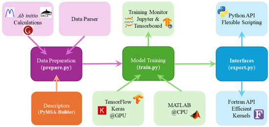
Figure 1. Schematic of the modules in the CQPES package. The workflow starts with File Parsing of the ab initio calculation results. The Data Preparation module then generates descriptors via PyMSA-Builder and standardizes the dataset. Model Training supports both GPU (TensorFlow/Keras) and CPU (MATLAB) backends, with real-time monitoring available via Jupyter or TensorBoard. Finally, the Interfaces module exports the model into two distinct APIs: the Python API for flexible scripting and interactive evaluation and the Fortran API which serves as efficient kernels for integrating with external dynamics software, e.g., Polyrate, VENUS, RPMDRate.

• PIP Basis Code Generation: Provides a code wrapper that facilitates the construction of Fortran code as a Python module, streamlining the development process.
• Dataset Preparation: Involves data generation and standardization and the division of datasets into subsets, such as training, testing, and validation sets, to ensure the accuracy and generalizability of the model.
• Model Training and Evaluation: Supports the training of PIP or PIP-NN models with the capability to monitor the training state in a web browser, enhancing the transparency and controllability of the training process.
• Model Exporting and Interfacing with Other Software: Allows for the inference of PIP-NN models in various programming environments including C/C++ (C99 and C++03 standard or newer), Fortran (Fortran 77 or newer), and Python (v3.8 or newer) This design enhances the applicability and flexibility of the models. Currently supports integration with a range of software such as Gaussian 16 [49], Polyrate 2017-C [50], VENUS96C [51], Caracal v1.1 [52], RPMDRate v2.0 [53], PyVibDMC 1.3.9 [54], etc., broadening the scope and functionality of the software.
• Active Learning Wrapper: Controls the progress of active learning and wraps training modules inside it. The history performance and the queried data points will be stored for checking the convergence and visualizing the space that the queried data points cover.

4.1. PIP Basis Code Generation

The MSA-2.0 software developed by Bowman’s group has been proved to be a robust and efficient protocol to generate PIP basis and easy-to-use Fortran code [42]. The monomial decomposition algorithm avoids redundant calculations of identical symmetric terms, achieving high efficiency. Since we introduced Python in the CQPES software to embrace the open-source community, the NumPy package, which is the fundamental package for scientific computing with Python, provides the f2py tool for compiling Fortran code as a Python module [55]. The PyMSA-Builder module was developed for these features.

4.2. Dataset Preparation

Upon completion of all quantum calculations using the chosen electronic structure method, the Cartesian coordinates and corresponding potential energies are extracted for subsequent standardization.

In CQPES, the module prepare.py will read a multi-frame xyz file, with the energy in Hartree and the Cartesian coordinates in angstrom. Then this module will calculate the PIPs of this configuration through the PyMSA-Builder model and calculate the potential energy by subtracting the reference energy E_ref from the electronic energy E and will convert it to eV.

$$V=\left(E-E_{\mathrm{ref}}\right)\times 27.2107$$

(19)

Usually, for a system with only a single well, E_ref is the energy of the stationary point. For reactions or interaction systems, E_ref is the energy of all of the species that are separated enough. The potential energy V is a relative value and will be used in later PES fitting.

Keywords for dataset preparation are listed in Table 1. The “xyz” specifies the path to a standard xyz file that contains the coordinates of all structures, and the electronic energy in Hartree can be stored in the comment line just above the coordinates of the structure. The “energy” is a plain text file with each line containing the electronic energy in the same order as in the xyz file, or, if it is “null”, the electronic energy will be read from the comment lines in the xyz file. The “ref_energy” specifies the reference energy of the system; “null” means the module will use the minimal energy. For a bimolecular system, the “ref_energy” is recommended to be the energy of all of the species that are separated enough. “alpha” is the range parameter in the Morse-like transformation, as shown in Equation (2) and defaults to 1.0 Å; for long-range interaction systems, increasing “alpha” may be beneficial. For instance, in the construction of a PES for the H₂ + NH₂⁻ reaction, a larger α value (2.1 Å) was adopted to ensure accuracy in the long-range asymptotic regions [56]. “output” indicates the directory to store pre-processed data, in which all data will be stored in NumPy’s npy format. Listing S1 is an example of a data preparation configuration.

Table 1. Keywords in dataset preparation.

Keyword	Brief Description
xyz	Path to raw data in xyz format
energy	Path to energy of corresponding structure in Hartree
ref_energy	Reference energy in Hartree
alpha	Range parameter in Morse-like transform
output	Path to npy format output

4.3. Model Training and Evaluation

The module train.py supports the creation of the NN part of PIP-NN and has the ability to train it from a single input file without any need to know how the code works. The NN is constructed in Keras, on top of Tensorflow [57,58]. To ensure the accuracy of the model, an open source Levenberg–Marquardt extension package for Tensorflow was employed as the optimizer. Currently, the module train.py has been tested on CPU and NVIDIA GPU platforms. The use of GPU does reduce time consumption. During the training, the real-time states can be monitored via Tensorboard in a web browser. After training, a Jupyter notebook template is available for analyzing the MAE (Mean Absolute Error), MSE (Mean Squared Error), and RMSE (Root Mean Squared Error) error of the training, testing, and validation subset and the entire dataset, or even plotting the fitting error distribution at the same time.

Table 2 shows the keywords for the training. The “data” key is the path to the packaged data as described in Table 1. The “network” key defines the number and size of hidden layers with the activation function; commonly, two hidden layers and the tanh activation function are suggested for our purpose. The “fit” contains the hyper-parameters for training: “lr” is the learning rate, “epoch” is the maximum number of epochs to train (500~2000 recommended), and “batch_size” is the mini-batch size. However, PIP-NNs trained with second order optimizers, especially Levenberg–Marquardt (LM), show better performance than first order optimizers. Thus, the hyper-parameters are tuned for the LM optimizer, which requires more data in one batch to estimate a better Hessian matrix. Setting “batch_size” as -1 means there is full-batch training. Options in the “lm” section control the LM optimization: “split” is the ratio of each subset, including training, validation, and test and “workdir” is the directory to save trained parameters and logs. Listing S2 is an example of a model training configuration.

Table 2. Keywords in model training.

Keyword	Brief Description
data	Path to npy format data
network
layers	Number of neurons in hidden layers
activation	Type of activation function
fit
lr	Learning rate
epoch	Maximum training epochs
batch_size	Number of samples per batch
lm	Detailed settings for Levenberg–Marquardt optimizer
split	Ratio of training, validation, and testing sets
workdir	Working directory of training

4.4. Model Exporting and Compatibility with Other Software

The trained model can be converted to either Keras’s HDF5 format or a plain text format. The latter is easy to parse in Fortran or Python and examples of calling trained models are available. The Fortran code is designed for computational efficiency, while the Python code is tailored for rapid script development and validation. For instance, the Python version of the PES can be invoked within Gaussian to expedite tasks such as optimization, frequency calculations, and IRC analysis, with the capability to visualize the results easily by GaussView 6 [59]. While, for large-scale molecular dynamics simulations on a refined PES, the Fortran version of the code can be integrated with dynamics software. We have validated this approach in software such as Polyrate 2017-C, VENUS96C, Caracal v1.1, RPMDRate v2.0, and PyVibDMC 1.3.9 [50,51,52,53].

In Table 3, the “train_config” is the path to the configuration file used in training for constructing the model. The “ckpt” is the path to the parameter checkpoint file. The “output” is the directory in which to save the exported model. Listing S3 is an example of a model exporting configuration.

Table 3. Keywords in exporting.

Keyword	Brief Description
train_config	Path to training configuration file
ckpt	Path to the training checkpoint
output	Path to save the exported model

An example input file to invoke the PES in Gaussian is shown in Listing S4. It includes geometry optimization, harmonic frequencies, and anharmonic frequencies analysis of a CH₄ molecule. There is no method or basis set in this file and an external PES Python script is used instead.

4.5. Active Learning Wrapper

The active learning wrapper provides two scripts. One performs the vote–query–train loop described in Figure 2 by calling voting functions and training functions; the other one can be used to parse the logs during active learning and visualize the history of the models’ performance, the projection of queried data points, and the fitting error scatter and histogram plots.

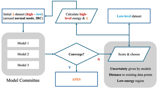
Figure 2. An active Δ machine learning workflow. It starts at a Δ dataset (difference between high-level and low-level) and it contains stationary points and some points along the normal modes and IRC for reactive systems. Models 1–3 are the members of the PIP-NN committee initialized with different random seeds. They are trained on the current dataset independently to estimate the prediction uncertainty. Then, the low-level dataset is scored and a subset is chosen for high-level labeling. By repeating this process the Δ dataset can be expanded. The active learning loop is considered converged when the Root Mean Squared Error (RMSE) of the model on the validation set stabilizes, in other words, the decrease is negligible after adding new points. The final ΔPES can be used in further simulations.

5. Applications

5.1. CH₄

The dataset for CH₄ was adopted from the VIB5 database with the energy computed at the CCSD(T)/cc-pVQZ level [60]. There are 97,271 points with energies less than 6.24 eV relative to the equilibrium. The C-H bond length ranges in 0.71~2.60 Å, and the H-C-H bond angle falls in 40.0–140.0°. For each training instance, the dataset was randomly divided into three subsets, named training (90%), validation (5%), and testing (5%).

The maximum order of PIP was chosen to be four, yielding 82 terms. Since the configurations in the dataset did not involve long-range interactions, the Morse-like range parameter α was fixed at 1.0 Å. After testing, two hidden layers, each with 20 neurons, are used with the tanh function as the activation function, resulting 2101 fitting parameters. The PIP-NN model was trained in two ways: one is the MATLAB code (R2020b) that was used in our previous works and the other one is the CQPES package in this work, powered by the Keras framework (Python v3.8, Keras v2.12.0, and TensorFlow v2.12.1), as shown in Figure 1. With MATLAB as the training engine, only the CPU is applicable. Note that Keras can benefit from the GPU.

The MAE and RMSE for each dataset are summarized in Table 4. The total RMSEs were 0.86 meV by CQPES and 0.81 meV by MATLAB, both of which are accurate enough. However, the training by CQPES was 2.3 times faster than by MATLAB, as shown in Table 5 and Figure 3. The scattered fitting error and the distribution of the absolute fitting errors by CQPES are shown in Figure 4a,b, respectively. As shown in Table 5 and Figure 3, the training on a 32-core CPU computing node spent ~1 h with MATLAB, but on an RTX 4090 GPU the current CQPES only took ~20 min. Besides this, several GPUs can be landed on a GPU computing node; one could train several PIP-NNs parallelly within a single node. The efficiency of the PIP-NN deployed by our previous Fortran code and by the ncnn-based implementation was compared (ncnn v20250916). The ncnn is a high-performance NN computing framework, which is highly optimized for mobile platforms, and also provides Streaming SIMD Extension (SSE) and Advanced Vector Extension (AVX, AVX2, and AVX512) acceleration instructions under x86-64 platforms [61]. This instruction set of acceleration technologies can improve the efficiency of linear algebra operations, thereby increasing the computational speed of NNs that involve a large number of matrix multiplications. The code was compiled by LLVM-based compilers inside the Intel oneAPI 2023 and ran on an Intel Core i9-13900KF CPU, providing extreme single-core performance. Calculating the energy of the whole CH₄ dataset, 97,271 points, took 0.19 s using previous code and 0.14 s using ncnn based code.

Table 4. Comparison of the fitting performance by CQPES and MATLAB for the CH₄ system.

Method	Dataset	MAE (meV)	RMSE (meV)
CQPES	Train	0.33	0.84
	Valid	0.37	1.19
	Test	0.34	0.91
	Total	0.34	0.86
MATLAB	Train	0.32	0.81
	Valid	0.36	0.95
	Test	0.33	0.97
	Total	0.32	0.82

Table 5. Training details for the CH₄, CH₃CN, and OH + CH₃OH systems. CQPES training was performed on an NVIDIA GeForce RTX 4090 GPU (24 GB VRAM), while MATLAB training used dual Intel Xeon E5-2682v4 CPUs (32 cores, 64 GB memory). For CQPES, a mini-batch strategy was adopted due to the GPU’s VRAM constraints.

System	Dataset	Network	Parameters	Method	Epochs	Wall Time (h)	RMSE (meV)
CH4	97,217	82-20-20-1	2101	CQPES	1000	0.33	0.86
				MATLAB	1000	1.08	0.81
CH3CN	30,974	1827-10-10-1	18,391	CQPES	211	1.23	2.85
				MATLAB	117	6.06	3.70
OH + CH3OH	140,192	419-20-80-1	10,161	CQPES	486	3.67	21.8
				MATLAB	607	27.66	18.8

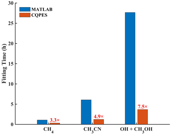
Figure 3. Comparison of the averaged fitting time by MATLAB and CQPES for the CH₄, CH₃CN, and OH + CH₃OH system.

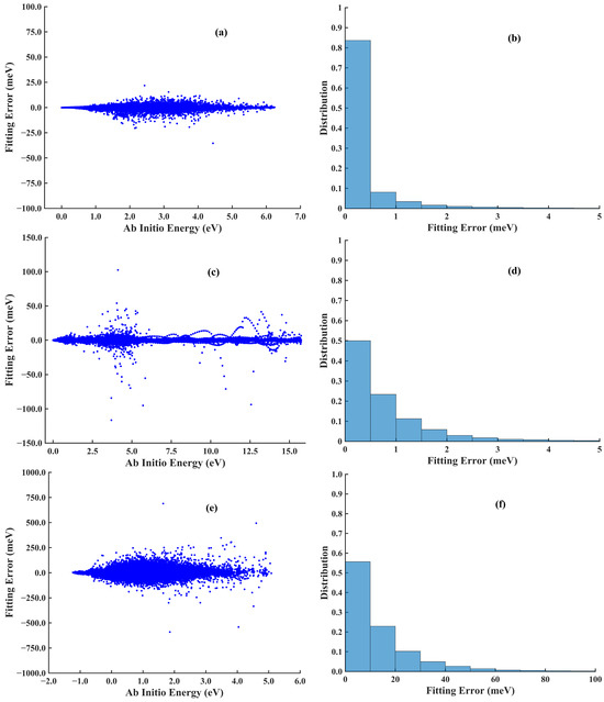
Figure 4. Scattered errors (left column) and distributions (right column) of the absolute errors of the (a,b) CH₄, (c,d) CH₃CN, and (e,f) OH + CH₃OH systems produced by CQPES.

Both methods predicted the correct T_d symmetry and the deviation of the C-H bond length from the ab initio calculation is of the order of 10⁻⁴ Å. Table 6 enumerates the energy, the harmonic or anharmonic vibrational frequencies of CH₄, and the vibrational zero-point energy (ZPE). Once again, the fitted PESs conform with the ab initio calculation. The deviations for the harmonic frequencies are generally less than 3 cm⁻¹. For ZPE, the deviation is only 0.01 kcal/mol. Anharmonic frequency analysis requires fourth derivatives of energy. Ab initio methods like CCSD(T), which lacks analytical high-order derivatives, are very time consuming: over 700 core-hours elapsed for the calculation performed at the frozen core CCSD(T)/cc-pVQZ level with CFOUR v2.1 [62], while the same calculation only took 3~4 s on the PES that is interfaced to Gaussian. The ZPE discrepancies between PES and ab initio results found that the ZPEs are within 0.01 kcal/mol. The anharmonic matrices are listed in Table 7. One can see that, although they are consistent with each other, apparent deviations do exist. The largest deviation is 6 cm⁻¹. Indeed, the comparison shows that the anharmonic matrices are more sensitive to the PES than the harmonic frequencies. The deviation can be attributed to the differences in the algorithm of the high-order numerical differentiation and the difference in the VPT2 algorithm implemented in the respective software packages. The VPT2 algorithm in CFOUR only calculates the full cubic force field with the semidiagonal part of the quartic force field, while VPT2 of Gaussian chooses the full quartic force field, which is more accurate; the frequencies of degenerate modes are reasonable.

Table 6. The electronic energy, harmonic vibrational frequencies, and ZPE of the stationary point CH₄ by the ab initio calculation and PESs.

Methods	E (a.u.)	Vibrational Frequencies (cm−1)										ZPE (kcal/mol)
Ab initio a	−40.450888	Harm	1345	1345	1345	1570	1570	3036	3157	3157	3157	28.14
		Anharm	1311	1311	1305	1533	1532	2911	3016	3013	3011	27.71
CQPES b	−40.450886	Harm	1345	1345	1345	1569	1569	3033	3157	3157	3157	28.13
		Anharm	1311	1311	1311	1534	1534	2916	3014	3014	3014	27.72
MATLAB c	−40.450887	Harm	1345	1345	1345	1570	1570	3036	3157	3157	3157	28.13
		Anharm	1311	1311	1311	1532	1532	2912	3013	3013	3013	27.71

^a Frozen core CCSD(T)/cc-pVQZ, CFOUR v2.1; ^b PIP-NN PES trained with CQPES; ^c PIP-NN PES trained with MATLAB code.

Table 7. A comparison of the anharmonic matrix of CH₄ by the PIP-NN PESs fitted by CQPES or MATLAB (cm⁻¹). The numbers 1–9 represent the indices of the vibrational modes of CH₄.

Vibrational Modes	1	2	3	4	5	6	7	8	9
CQPES	−5.26
	−4.91	−7.00
	−5.39	1.55	−6.88
	−4.59	−4.86	−5.64	0.49
	−5.47	−5.20	−4.42	−0.57	0.49
	0.59	0.59	0.59	−16.84	−16.84	−9.54
	−8.76	−8.08	−9.21	−11.09	−14.93	−54.40	−25.70
	−8.36	−9.65	−8.03	−14.61	−11.41	−54.40	−47.26	−27.44
	−8.92	−8.32	−8.79	−13.33	−12.69	−54.41	−30.12	−23.20	−31.73
MATLAB	−5.37
	−3.21	−6.01
	−5.83	−3.26	−5.36
	−11.59	−1.10	−4.12	−0.18
	0.38	−10.11	−7.09	−1.29	−0.18
	−1.05	−1.05	−1.05	−18.65	−18.65	−11.98
	−8.63	−8.45	−7.90	−14.02	−11.78	−53.25	−31.66
	−8.24	−8.14	−8.60	−12.52	−13.28	−53.26	−31.92	−34.89
	−8.10	−8.39	−8.47	−12.16	−13.64	−53.27	−25.54	−12.64	−36.49

5.2. CH₃CN System

There exists only one isomerization reaction pathway between CH₃NC and CH₃CN, and the corresponding PES should comprehensively describe the reaction path that includes these two molecules and the transition state. Namely, the methyl group rotates around the cyano group. The dataset of this system was taken from ref. [63], which includes 30,974 data points calculated by CCSD(T)-F12a. The fifth-order PIPs, including 1826 terms, along with 10 neurons in the first and second hidden layers, are used, yielding 18,391 parameters. The final RMSEs are 3.70 meV, calculated by MATLAB and 2.84 meV, calculated by CQPES. This error is extremely small (much less than 1 kcal/mol). Since the reaction rate depends exponentially on the barrier height, this high fitting precision is critical for the subsequent kinetic studies. Table 5 and Figure 3 show that the current training is 3.9 times faster than previous MATLAB fitting. Figure 4c,d depict the scattered plot and the histogram of the absolute fitting error. Then, this PES created by CQPES is interfaced with the Caracal software, which supports calculating the rate of unimolecular isomerization by the ring polymer molecular dynamics (RPMD) approach [52].

To integrate with the Caracal software, three functions are exported in the interface: loading the trained parameters from the files and initializing the NN, calculating the potential energy of the input Cartesian coordinates, and calculating the gradient of the potential energy with respect to the Cartesian coordinates, or Cartesian force. The Caracal software allows users to add their PESs to the software. The PESs can be compiled with Caracal for efficiency. The cost of exchanging the Cartesian coordinates and potential energy with forces between PESs and MD engines would never be the bottleneck. RPMD calculation of the PES for the isomerization of CH₃CN produced accurate reaction rate coefficients, which are in good agreement with the experimental results at the energy range of 472.55~532.92 K. This agreement validates the quality of the PES. It shows that the model reproduces the ab initio energy and forces well. Consequently, the CQPES interface ensures reliable dynamics trajectories, leading to reasonable kinetic results comparable to experiments. Additionally, the intramolecular energy transfers were studied with the PES interfaced to VENUS96C. Detailed results and discussions are demonstrated in ref [63].

5.3. OH + CH₃OH System

The OH + CH₃OH system has 8 atoms and its degrees of freedom are 16. Recently, both PIP and Fundamental Invariant (FI) descriptors were used to develop its full-dimensional accurate PES by PIP-NN and FI-NN [64,65,66,67,68]. Only 419 FIs are sufficient for FI-NN, much less than the 3059 PIPs in PIP-NN PES. There are 10,161 parameters in the FI-NN, which contains 419 FIs as input, 20 neurons for the first hidden layer, 80 neurons for the second hidden layer, and 1 for the output layer. The FI-NN was featured with the implementation of the analytical gradient and the migration of the NN part to the MKL backend, which collectively sped up the molecular dynamics simulation 10-fold [37,69]. However, the training of the NN necessitates a substantial amount of time, and the previous MATLAB code was only executable on a CPU, thereby precluding the benefits of GPU acceleration.

In this work, CQPES solves this training problem. Since CQPES is modular, FIs can be easily integrated by replacing the descriptor module in prepare.py. Furthermore, the NN training progress can be accelerated by Keras with GPU support. The training details are listed in Table 5. Training with MATLAB code converged at 607 epochs, spending 27.66 h on a 32-core CPU computing node, resulting in 885 core-hours in total. The training on an RTX 4090 GPU by CQPES reduced the training time to 3 h and 40 min within 486 epochs. The current fitting is 6.5 times faster, as shown in Table 5 and Figure 3, which also clearly indicates that as the size of system and dataset increases, switching to GPU-based training code can significantly reduce the time consumption. Both NNs are accurate enough to reproduce the potential energy of this complex system; the total RMSEs are 18.8 meV by MATLAB and 21.8 meV by CQPES. Figure 4e,f corresponds to the scatter plot and histogram of fitting error. This massive speed-up, from days to hours, proves the advantage of the GPU backend. This is especially important for high-dimensional systems with large datasets. It shows that CQPES solves the training bottleneck for complex reactive surfaces.

5.4. Ar + H₂O System

The accurate description of the weak interactions inside the Van der Waals complex, such as Ar + H₂O, is important to simulating its rotational and vibrational spectrum, and accurate PESs at the CCSD(T) level are often needed [70]. In this case, a Δ-ML method is used to improve the PES from low-level to high-level. The low-level method is B3LYP-D3(BJ)/AVTZ, after testing, and the high-level method is CCSD(T)-F12a/AVTZ. Compared with the high-level method, the B3LYP-D3(BJ) can yield reasonably complex and intramolecular potential energy curves. The low-level dataset is sampled by normal mode displacements, rigid scan grids, and quasiclassical trajectory dynamics, and 32,524 data points in total were sampled. After testing, the NN architecture of the low-level PES is 49-30-40-1. The RMSE is 0.039 meV. The scatter plot and histogram of the absolute fitting error are shown in Figure 5a,b. The process for training the Δ PES is described in Figure 2, it started from sampling around the stationary point along the normal mode displacements and covered the structure space by adding other data points step by step. In each query, 100 data points were voted by inspecting performances from three independent models. After 20 queries, the Δ dataset contained 2000 (~6%) data points in the low-level dataset.

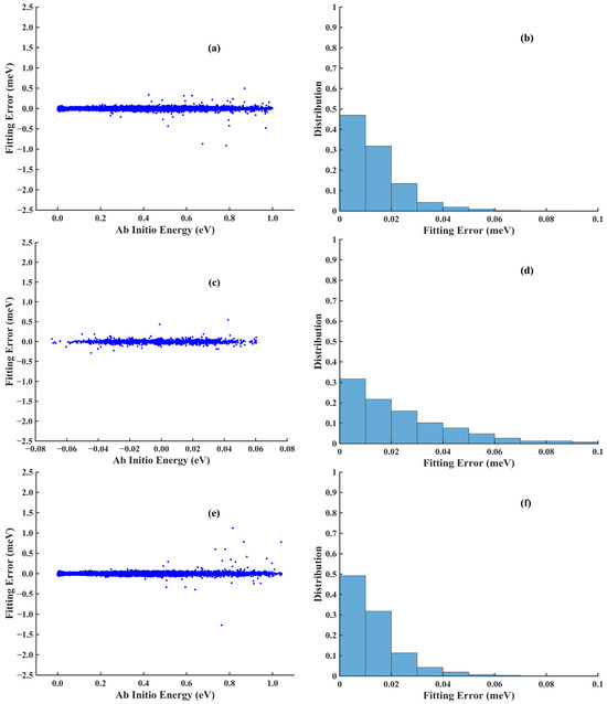
Figure 5. Scatter plots (left column) and distributions (right column) of the absolute errors of the (a,b) low-level PES, (c,d) ΔPES, and (e,f) high-level PES for the H₂O-Ar system.

Figure 6a shows the projection of the selected 2000 data points over low-level energy verses high- and low-energy differences. Figure 6b depicts the low-level sampling data points and the selected high-level sampling data points along the Ar-O distance. Figure 6c depicts the history of the mean and minimum RMSE from the 3 models as more data points were added for the high-level training. At the end of active learning, the mean and minimum RMSE no longer decreased. The final RMSE of the Δ PES is 0.039 meV under NN architecture 49-15-15-1. Figure 5c,d shows the scatter plot of the error and the histogram of the absolute fitting error, respectively. Then, the high-level potential energy for the remaining data points can be estimated by summing the results by the low-level PES and the Δ PES; V_low + V_high-low. Finally, the high-level PES shares the same architecture as the low-level PES and the fitting error is 0.022 meV. The scatter plot and the histogram of the fitting error are shown in Figure 5e,f, respectively.

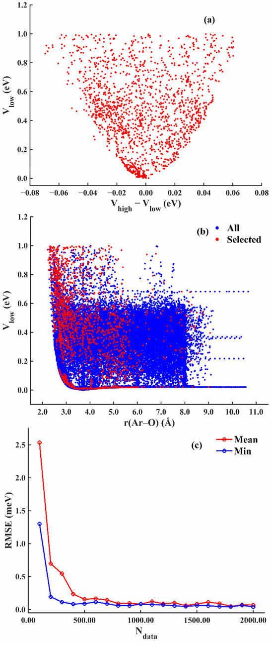
Figure 6. H₂O-Ar system: (a) Distribution of DFT energy vs. energy difference in selected data points. (b) Projection of selected data points over distance between Ar and O atom. (c) The mean and minimum RMSE vs. the number of queried data points during the active learning process.

The Ar + H₂O case proves that the active learning module is very efficient. By picking points with high uncertainty, it avoids redundant calculations. Therefore, it requires much fewer high-level ab initio points than grid sampling.

6. Conclusions and Outlook

In this work, we presented the CQPES software package along with four representative cases. CQPES consists of modules for data preparation, PIP-NN training, evaluation, and interfaces to other software. The modular design makes the package user-friendly. For example, users can replace PIP descriptors with Fundamental Invariants (FIs), or switch back to the CPU platform during training. The combination of Python and Fortran allows users to check PESs easily and to simulate efficient dynamics. Also, the interfaces allow direct connection to external software.

However, the method has limitations. The PIP-NN approach is mainly effective for small-to-medium systems (typically less than 10 atoms). For larger systems, the number of basis functions increases too quickly, making the calculation very expensive. This leads us to consider incorporating fragment PIP descriptors or more efficient Fundamental Invariants (FIs) into CQPES.

For future development, we aim to achieve end-to-end automation. We plan to adopt a layered design, similar to the relationship between Keras and TensorFlow. The low-level code implements the specific details of sampling and fitting. This allows advanced users to learn the algorithm details or carry out further development on top of it. Currently, the low-level workflow serves as a tutorial demo. The high-level API (under development) will allow users to freely combine modules to meet their needs. We have made the source code public to the community. We hope it helps to accelerate the construction of accurate PESs. We will continue to refine the package by adding new features and incorporating our group’s experience in molecular dynamics simulations.

References

- Dawes, R.; Ndengué, S.A. Single- and multireference electronic structure calculations for constructing potential energy surfaces. Int. Rev. Phys. Chem. 2016, 35, 441–478. [Google Scholar] [CrossRef]
- Fu, B.; Zhang, D.H. Ab Initio Potential Energy Surfaces and Quantum Dynamics for Polyatomic Bimolecular Reactions. J. Chem. Theory Comput. 2018, 14, 2289–2303. [Google Scholar] [CrossRef]
- Qu, C.; Yu, Q.; Bowman, J.M. Permutationally Invariant Potential Energy Surfaces. Annu. Rev. Phys. Chem. 2018, 69, 151–175. [Google Scholar] [CrossRef]
- Manzhos, S.; Carrington, T. Neural Network Potential Energy Surfaces for Small Molecules and Reactions. Chem. Rev. 2021, 121, 10187–10217. [Google Scholar] [CrossRef]
- Bowman, J.M.; Qu, C.; Conte, R.; Nandi, A.; Houston, P.L.; Yu, Q. A perspective marking 20 years of using permutationally invariant polynomials for molecular potentials. J. Chem. Phys. 2025, 162, 180901. [Google Scholar] [CrossRef]
- Bowman, J.M.; Czakó, G.; Fu, B. High-dimensional ab initio potential energy surfaces for reaction dynamics calculations. Phys. Chem. Chem. Phys. 2011, 13, 8094–8111. [Google Scholar] [CrossRef] [PubMed]
- Chen, J.; Xu, X.; Xu, X.; Zhang, D.H. Communication: An accurate global potential energy surface for the OH + CO → H + CO2 reaction using neural networks. J. Chem. Phys. 2013, 138, 221104. [Google Scholar] [CrossRef] [PubMed]
- Chen, J.; Xu, X.; Zhang, D.H. A global potential energy surface for the H2 + OH ↔ H2O + H reaction using neural networks. J. Chem. Phys. 2013, 138, 154301. [Google Scholar] [CrossRef] [PubMed]
- Jiang, B.; Guo, H. Permutation invariant polynomial neural network approach to fitting potential energy surfaces. J. Chem. Phys. 2013, 139, 054112. [Google Scholar] [CrossRef]
- Li, J.; Jiang, B.; Guo, H. Permutation invariant polynomial neural network approach to fitting potential energy surfaces. II. Four-atom systems. J. Chem. Phys. 2013, 139, 204103. [Google Scholar] [CrossRef]
- Lu, D.; Li, J. Full-dimensional global potential energy surfaces describing abstraction and exchange for the H + H2S reaction. J. Chem. Phys. 2016, 145, 014303. [Google Scholar] [CrossRef]
- Li, J.; Varga, Z.; Truhlar, D.G.; Guo, H. Many-Body Permutationally Invariant Polynomial Neural Network Potential Energy Surface for N4. J. Chem. Theory Comput. 2020, 16, 4822–4832. [Google Scholar] [CrossRef] [PubMed]
- Shao, K.; Chen, J.; Zhao, Z.; Zhang, D.H. Communication: Fitting potential energy surfaces with fundamental invariant neural network. J. Chem. Phys. 2016, 145, 071101. [Google Scholar] [CrossRef] [PubMed]
- Hao, Y.; Lu, X.; Fu, B.; Zhang, D.H. New Algorithms to Generate Permutationally Invariant Polynomials and Fundamental Invariants for Potential Energy Surface Fitting. J. Chem. Theory Comput. 2025, 21, 1046–1053. [Google Scholar] [CrossRef] [PubMed]
- Hollebeek, T.; Ho, T.-S.; Rabitz, H. Constructing multidimensional molecular potential energy surfaces from ab initio data. Annu. Rev. Phys. Chem. 1999, 50, 537–570. [Google Scholar] [CrossRef]
- Bartók, A.P.; Csányi, G. Gaussian approximation potentials: A brief tutorial introduction. Int. J. Quantum Chem. 2015, 115, 1051–1057. [Google Scholar] [CrossRef]
- Qu, C.; Yu, Q.; Van Hoozen, B.L.; Bowman, J.M.; Vargas-Hernández, R.A. Assessing Gaussian Process Regression and Permutationally Invariant Polynomial Approaches To Represent High-Dimensional Potential Energy Surfaces. J. Chem. Theory Comput. 2018, 14, 3381–3396. [Google Scholar] [CrossRef]
- Liu, Y.; Guo, H. A Gaussian Process Based Δ-Machine Learning Approach to Reactive Potential Energy Surfaces. J. Phys. Chem. A 2023, 127, 8765–8772. [Google Scholar] [CrossRef]
- Jiang, B.; Li, J.; Guo, H. High-Fidelity Potential Energy Surfaces for Gas-Phase and Gas–Surface Scattering Processes from Machine Learning. J. Phys. Chem. Lett. 2020, 11, 5120–5131. [Google Scholar] [CrossRef]
- Raff, L.M.; Malshe, M.; Hagan, M.; Doughan, D.I.; Rockley, M.G.; Komanduri, R. Ab initio potential-energy surfaces for complex, multichannel systems using modified novelty sampling and feedforward neural networks. J. Chem. Phys. 2005, 122, 084104. [Google Scholar] [CrossRef]
- Jiang, B.; Li, J.; Guo, H. Potential Energy Surfaces from High Fidelity Fitting of Ab Initio Points: The Permutation Invariant Polynomial Neural Network Approach. Int. Rev. Phys. Chem. 2016, 35, 479. [Google Scholar] [CrossRef]
- Jose, K.V.J.; Artrith, N.; Behler, J. Construction of high-dimensional neural network potentials using environment-dependent atom pairs. J. Chem. Phys. 2012, 136, 194111. [Google Scholar] [CrossRef]
- Behler, J. Constructing high-dimensional neural network potentials: A tutorial review. Int. J. Quantum Chem. 2015, 115, 1032–1050. [Google Scholar] [CrossRef]
- Uteva, E.; Graham, R.S.; Wilkinson, R.D.; Wheatley, R.J. Active learning in Gaussian process interpolation of potential energy surfaces. J. Chem. Phys. 2018, 149, 174114. [Google Scholar] [CrossRef]
- Lin, Q.; Zhang, L.; Zhang, Y.; Jiang, B. Searching Configurations in Uncertainty Space: Active Learning of High-Dimensional Neural Network Reactive Potentials. J. Chem. Theory Comput. 2021, 17, 2691–2701. [Google Scholar] [CrossRef]
- Shuaibi, M.; Sivakumar, S.; Chen, R.Q.; Ulissi, Z.W. Enabling robust offline active learning for machine learning potentials using simple physics-based priors. Mach. Learn. Sci. Technol. 2020, 2, 025007. [Google Scholar] [CrossRef]
- Győri, T.; Czakó, G. Automating the development of high-dimensional reactive potential energy surfaces with the ROBOSURFER program system. J. Chem. Theory Comput. 2020, 16, 51–66. [Google Scholar] [CrossRef]
- Czakó, G.; Győri, T.; Papp, D.; Tajti, V.; Tasi, D.A. First-Principles Reaction Dynamics beyond Six-Atom Systems. J. Phys. Chem. A 2021, 125, 2385–2393. [Google Scholar] [CrossRef]
- Abbott, A.S.; Turney, J.M.; Zhang, B.; Smith, D.G.A.; Altarawy, D.; Schaefer, H.F. PES-Learn: An Open-Source Software Package for the Automated Generation of Machine Learning Models of Molecular Potential Energy Surfaces. J. Chem. Theory Comput. 2019, 15, 4386–4398. [Google Scholar] [CrossRef] [PubMed]
- Quintas-Sánchez, E.; Dawes, R. AUTOSURF: A Freely Available Program To Construct Potential Energy Surfaces. J. Chem. Inf. Model. 2019, 59, 262–271. [Google Scholar] [CrossRef] [PubMed]
- Töpfer, K.; Vazquez-Salazar, L.I.; Meuwly, M. Asparagus: A Toolkit for Autonomous, User-Guided Construction of Machine-Learned Potential Energy Surfaces. arXiv 2024, arXiv:2407.15175. [Google Scholar] [CrossRef]
- Hjorth Larsen, A.; Jørgen Mortensen, J.; Blomqvist, J.; Castelli, I.E.; Christensen, R.; Dułak, M.; Friis, J.; Groves, M.N.; Hammer, B.; Hargus, C.; et al. The atomic simulation environment—A Python library for working with atoms. J. Phys. Condens. Matter 2017, 29, 273002. [Google Scholar] [CrossRef]
- Brooks, B.R.; Brooks, C.L., III; Mackerell, A.D., Jr.; Nilsson, L.; Petrella, R.J.; Roux, B.; Won, Y.; Archontis, G.; Bartels, C.; Boresch, S.; et al. CHARMM: The biomolecular simulation program. J. Comput. Chem. 2009, 30, 1545–1614. [Google Scholar] [CrossRef]
- Buckner, J.; Liu, X.; Chakravorty, A.; Wu, Y.; Cervantes, L.F.; Lai, T.T.; Brooks, C.L., III. pyCHARMM: Embedding CHARMM Functionality in a Python Framework. J. Chem. Theory Comput. 2023, 19, 3752–3762. [Google Scholar] [CrossRef] [PubMed]
- Song, K.; Käser, S.; Töpfer, K.; Vazquez-Salazar, L.I.; Meuwly, M. PhysNet meets CHARMM: A framework for routine machine learning/molecular mechanics simulations. J. Chem. Phys. 2023, 159, 024125. [Google Scholar] [CrossRef]
- Li, J.; Liu, Y. Data Quality, Data Sampling and Data Fitting: A Tutorial Guide for Constructing Full-Dimensional Accurate Potential Energy Surfaces (PESs) of Molecules and Reactions. Mach. Learn. Mol. Sci. 2023, 36, 161–201. [Google Scholar]
- Shang, C.; Zhang, D. Analytical Gradient Method for Fundamental Invariant Neural Networks. Chem. J. Chin. Univ. 2021, 42, 2146–2154. [Google Scholar]
- Battiti, R. First-and second-order methods for learning: Between steepest descent and Newton’s method. Neural Comput. 1992, 4, 141–166. [Google Scholar] [CrossRef]
- Dennis, J.E., Jr.; Schnabel, R.B. Numerical Methods for Unconstrained Optimization and Nonlinear Equations; SIAM: Philadelphia, PA, USA, 1996. [Google Scholar]
- Floudas, C.A.; Pardalos, P.M. Encyclopedia of Optimization; Springer Science & Business Media: Berlin/Heidelberg, Germany, 2008. [Google Scholar]
- Glorot, X.; Bordes, A.; Bengio, Y. Deep sparse rectifier neural networks. In Proceedings of the Fourteenth International Conference on Artificial Intelligence and Statistics, Ft. Lauderdale, FL, USA, 11–13 April 2011; pp. 315–323. [Google Scholar]
- Nandi, A.; Qu, C.; Bowman, J.M. Using Gradients in Permutationally Invariant Polynomial Potential Fitting: A Demonstration for CH4 Using as Few as 100 Configurations. J. Chem. Theory Comput. 2019, 15, 2826–2835. [Google Scholar] [CrossRef] [PubMed]
- Ge, F.; Wang, R.; Qu, C.; Zheng, P.; Nandi, A.; Conte, R.; Houston, P.L.; Bowman, J.M.; Dral, P.O. Tell Machine Learning Potentials What They Are Needed For: Simulation-Oriented Training Exemplified for Glycine. J. Phys. Chem. Lett. 2024, 15, 4451–4460. [Google Scholar] [CrossRef]
- Peslherbe, G.H.; Wang, H.; Hase, W.L. Monte Carlo sampling for classical trajectory simulations, a chapter in Monte Carlo methods in chemical physics. Adv. Chem. Phys. 1999, 105, 171–201. [Google Scholar]
- Liu, Y.; Li, J. Permutation-Invariant-Polynomial Neural-Network-Based Δ-Machine Learning Approach: A Case for the HO2 Self-Reaction and Its Dynamics Study. J. Phys. Chem. Lett. 2022, 13, 4729–4738. [Google Scholar] [CrossRef]
- Song, K.; Li, J. The neural network based Δ-machine learning approach efficiently brings the DFT potential energy surface to the CCSD(T) quality: A case for the OH + CH3OH reaction. Phys. Chem. Chem. Phys. 2023, 25, 11192–11204. [Google Scholar] [CrossRef] [PubMed]
- Behler, J. Neural network potential-energy surfaces in chemistry: A tool for large-scale simulations. Phys. Chem. Chem. Phys. 2011, 13, 17930–17955. [Google Scholar] [CrossRef]
- Lin, Q.; Zhang, Y.; Zhao, B.; Jiang, B. Automatically growing global reactive neural network potential energy surfaces: A trajectory-free active learning strategy. J. Chem. Phys. 2020, 152, 154104. [Google Scholar] [CrossRef]
- Frisch, M.J.; Trucks, G.W.; Schlegel, H.B.; Scuseria, G.E.; Robb, M.A.; Cheeseman, J.R.; Scalmani, G.; Barone, V.; Petersson, G.A.; Nakatsuji, H.; et al. Gaussian 16; Rev. C.01; Gaussian Inc.: Wallingford, CT, USA, 2016. [Google Scholar]
- Meana-Pañeda, R.; Zheng, J.; Bao, J.L.; Zhang, S.; Lynch, B.J.; Corchado, J.C.; Chuang, Y.-Y.; Fast, P.L.; Hu, W.-P.; Liu, Y.-P.; et al. Polyrate 2023: A computer program for the calculation of chemical reaction rates for polyatomics. New version announcement. Comput. Phys. Commun. 2024, 294, 108933. [Google Scholar] [CrossRef]
- Hase, W.L.; Duchovic, R.J.; Hu, X.; Komornicki, A.; Lim, K.F.; Lu, D.-H.; Peslherbe, G.H.; Swamy, K.N.; Linde, S.R.V.; Varandas, A.; et al. VENUS96: A General Chemical Dynamics Computer Program. Quantum Chem. Program Exch. Bull. 1996, 16, 671. [Google Scholar]
- Steffen, J. Caracal: A Versatile Ring Polymer Molecular Dynamics Simulation Package. J. Chem. Theory Comput. 2023, 19, 5334–5355. [Google Scholar] [CrossRef]
- Suleimanov, Y.V.; Allen, J.W.; Green, W.H. RPMDrate: Bimolecular chemical reaction rates from ring polymer molecular dynamics. Comput. Phys. Comm. 2013, 184, 833–840. [Google Scholar] [CrossRef]
- DiRisio, R.; Lu, F.; Moonkaen, M. rjdirisio/pyvibdmc: Excited State Importance Sampling Patch; Zenodo: Geneva, Switzerland, 2024. [Google Scholar]
- Harris, C.R.; Millman, K.J.; van der Walt, S.J.; Gommers, R.; Virtanen, P.; Cournapeau, D.; Wieser, E.; Taylor, J.; Berg, S.; Smith, N.J.; et al. Array programming with NumPy. Nature 2020, 585, 357–362. [Google Scholar] [CrossRef] [PubMed]
- Song, K.; Song, H.; Li, J. Validating experiments for the reaction H2 + NH2− by dynamical calculations on an accurate full-dimensional potential energy surface. Phys. Chem. Chem. Phys. 2022, 24, 10160–10167. [Google Scholar] [CrossRef]
- Chollet, F. Keras: The Python Deep Learning Library; 2018; p. ascl:1806.1022. Available online: https://ui.adsabs.harvard.edu/abs/2018ascl.soft06022C/abstract (accessed on 10 December 2025).
- Singh, P.; Manure, A. Introduction to TensorFlow 2.0. In Learn TensorFlow 2.0: Implement Machine Learning and Deep Learning Models with Python; Apress: Berkeley, CA, USA, 2020; pp. 1–24. [Google Scholar]
- Dennington, R.; Keith, T.A.; Millam, J.M. GaussView, Version 6; Semichem Inc.: Shawnee Mission, KS, USA, 2016.
- Zhang, L.; Zhang, S.; Owens, A.; Yurchenko, S.N.; Dral, P.O. VIB5 database with accurate ab initio quantum chemical molecular potential energy surfaces. Sci. Data 2022, 9, 84. [Google Scholar] [CrossRef]
- Ni, H.; The ncnn contributors. ncnn; Tencent Holdings Ltd.: Shenzhen, China, 2017. [Google Scholar]
- Matthews, D.A.; Cheng, L.; Harding, M.E.; Lipparini, F.; Stopkowicz, S.; Jagau, T.-C.; Szalay, P.G.; Gauss, J.; Stanton, J.F. Coupled-cluster techniques for computational chemistry: The CFOUR program package. J. Chem. Phys. 2020, 152, 214108. [Google Scholar] [CrossRef]
- Li, J.; Li, J.; Li, J. Full-dimensional accurate potential energy surface and dynamics for the unimolecular isomerization reaction CH3NC ⇌ CH3CN. J. Chem. Phys. 2025, 162, 014305. [Google Scholar] [CrossRef]
- Lu, X.; Li, L.; Zhang, X.; Fu, B.; Xu, X.; Zhang, D.H. Dynamical Effects of SN2 Reactivity Suppression by Microsolvation: Dynamics Simulations of the F–(H2O) + CH3I Reaction on a 21-Dimensional Potential Energy Surface. J. Phys. Chem. Lett. 2022, 13, 5253–5259. [Google Scholar] [CrossRef]
- Lu, X.; Shang, C.; Li, L.; Chen, R.; Fu, B.; Xu, X.; Zhang, D.H. Unexpected steric hindrance failure in the gas phase F− + (CH3)3CI SN2 reaction. Nat. Commun. 2022, 13, 4427. [Google Scholar] [CrossRef]
- Lu, D.; Li, J.; Guo, H. Comprehensive Investigations of the Cl + CH3OH → HCl + CH3O/CH2OH Reaction: Validation of Experiment and Dynamic Insights. CCS Chem. 2020, 2, 882–894. [Google Scholar] [CrossRef]
- Lu, D.; Behler, J.; Li, J. Accurate Global Potential Energy Surfaces for the H + CH3OH Reaction by Neural Network Fitting with Permutation Invariance. J. Phys. Chem. A 2020, 124, 5737–5745. [Google Scholar] [CrossRef] [PubMed]
- Weichman, M.L.; DeVine, J.A.; Babin, M.C.; Li, J.; Guo, L.; Ma, J.; Guo, H.; Neumark, D.M. Feshbach resonances in the exit channel of the F + CH3OH → HF + CH3O reaction observed using transition-state spectroscopy. Nat. Chem. 2017, 9, 950–955. [Google Scholar] [CrossRef] [PubMed]
- Song, K.; Li, J. Fundamental Invariant Neural Network (FI-NN) Potential Energy Surface for the OH + CH3OH Reaction with Analytical Forces. J. Phys. Chem. A 2024, 128, 6636–6647. [Google Scholar] [CrossRef]
- Liu, Q.; Wang, J.; Zhou, Y.; Xie, D. A full-dimensional ab initio intermolecular potential energy surface and dipole moment surfaces for H2O-Ar. Curr. Chin. Sci. 2022, 2, 325–334. [Google Scholar] [CrossRef]
Disclaimer/Publisher’s Note: The statements, opinions and data contained in all publications are solely those of the individual author(s) and contributor(s) and not of MDPI and/or the editor(s). MDPI and/or the editor(s) disclaim responsibility for any injury to people or property resulting from any ideas, methods, instructions or products referred to in the content. |
© 2025 by the authors. Licensee MDPI, Basel, Switzerland. This article is an open access article distributed under the terms and conditions of the Creative Commons Attribution (CC BY) license (https://creativecommons.org/licenses/by/4.0/).