Abstract
Composting can be perceived as an art and science of converting organic waste into a rich and nutritious soil amendment—compost. The existing literature talks about how and what parameters need to be monitored in the process of composting and what actions are to be taken to optimize the process. In this paper, the development, deployment and data analytics of a compost monitoring system are presented, wherein not only the parameters to be measured but also the topology, mechanical design and battery operation details, which are crucial for the deployment of the system, are considered. Having realized that the temperature plays an important role in the process of composting, a contactless method of monitoring the compost temperature, using thermal imaging, has been investigated. Results showing the screenshots of the successfully developed system, plots of the obtained data and the inferences drawn from them are presented. This work not only contributes to the composting data, which is scarce, but also brings out the advantages of using thermal images in addition to temperature sensor probes.
1. Introduction
Composting is the process of decomposing organic material into ‘compost’ that can be recycled as a fertilizer and soil supplement. Organic wastes from kitchens and gardens are converted over time into a nutrient-rich, humus-like substance called compost by the action of microorganisms, fungi and other decomposers. Adding compost to the soil can improve soil fertility. It can also reduce the requirement of chemical fertilizers, help soil retain moisture, reduce plant infestations, etc. Additionally, composting reduces the waste that enters the landfills. When organic wastes decompose anaerobically in landfills, it produces methane, a potent greenhouse gas, which could be hazardous to the environment, and this can be minimized by composting [].
The composting process starts with the filling of the bin, balancing brown and green organic waste materials layer wise, thus maintaining the carbon to nitrogen ratio for promoting effective decomposition. Subsequently, a maggot-attracting powder containing attractants for black soldier flies is added. This procedure is commonly practiced in South Asia. The flies lay eggs that develop into maggots. This process generates heat. Then, the decomposition process continues through the action of maggots, microbes and other decomposers. Lack of sufficient oxygen can create anaerobic pockets, slowing down the decomposition and potentially creating odors. Cocoa powder is added to form a layer of organic material that is not consumed by the maggots, allowing the compost below to stabilize and prevent maggots from coming to the surface. The addition of cocoa powder is a local practice performed in the southern states of India. It also controls the unpleasant odors from emanating. The microbial activity continues to bio converse any remaining organic matter, resulting in a nutrient-rich compost. Once the compost is fully matured, it is harvested [,].
As it can be seen, composting is an intricate and involved process which needs periodic monitoring to ensure the right conditions for microorganisms and insects to efficiently break down organic matter. Apartment complexes, gated communities and campuses are adopting community composting. Automation of monitoring in such scenarios reduces the need of periodic checks by personnel involved. The human involvement after filling the bin can be only based on alerts, thus reducing the cumbersome task of physically checking on the compost status. Monitoring of compost is crucial for several reasons. It needs to be ensured that the right conditions for microorganisms and insects to efficiently break down organic matter are maintained. Appropriate temperatures need to be maintained to speed up decomposition and kill pathogens. The moisture levels need to be maintained to prevent the compost from becoming too dry or too wet, which can hinder the decomposition process. Sufficient aeration to support aerobic decomposition and prevent foul odors from anaerobic processes needs to be ensured. Maintaining the right carbon-to-nitrogen ratio to ensure effective decomposition and high-quality compost is also essential. IoT-enabled monitoring without human intervention scales up the composting operations, making it viable for large institutions like colleges, municipalities and farms.
Most of the earlier academic work in this area focuses on the basic process of the composting and alert generation. In comparison, our focus in this paper is on the system architecture of an IoT-enabled remote compost monitoring system, involving development of a prototype for the deployment scenario of apartment complexes, gated communities and campuses. Electronics used in developing the prototype, battery operation and mechanical design details of the system are described. The compost monitoring is performed by using a set of sensors in the form of probes to measure temperature, moisture, pH, etc., assembled as a sensor hub. Sensors to measure gas concentrations like ammonia, hydrogen sulfide and methane are added to the hub.
The sensor hub is mounted inside the bin, and the probes need to be inserted into the compost. Information obtained from the probe inserted gives the measurements at and around the place of insertion. This approach lacks in spatially distributed data of the biomass, which is required to ensure an efficient composting process. Usage of thermal cameras allows non-invasive measurement of temperature that can make thermal imaging in composting research and production viable. They have the advantage of providing the spatial information of the temperature across the bin.
2. Literature Survey
Compost monitoring and automation has been discussed in the literature. In [], a prototype of a domestic smart composter is presented by combining the ad hoc design of a multi-sensor electronic board and microwave imaging technique. [] describes a system to monitor the temperature, humidity, waste crushing process and chopper condition. In [], bio-waste composting was monitored for obtaining temperature, moisture and oxygen content. [] discusses monitoring of the vermi-composting process. In [], the system described has an installation of sensors in a rotary drum, which measure temperature, humidity, ammonia level and pH. The measured values are communicated wirelessly to the application. [] introduces the concept of COMPosting as a Service (COMPaaS). Composting machinery is equipped with sensors, whose measurements are communicated to cloud services. The cloud services perform real-time data analysis and instruct the composting machinery to perform the appropriate actions based on the outcome of the analysis. [] presents the development and implementation of a compost monitoring system wherein the field conditions at the farm are considered. In [], the temperature, humidity, gas and moisture levels of the compost are monitored with the help of Arduino, Node MCU and various sensors. A smart composting apparatus is discussed in [], consisting of a bin, an access panel, an aerator, a water content sensor, a valve and a composting controller. [,] present a system and method for monitoring a network of IoT composting end-devices comprising one or more compost bins, remote monitoring devices and personal user devices. The data is also posted on a public forum to track and encourage community composting. [] presents an IoT-based agricultural compost monitoring system composed of sensor probes, edge and cloud platforms and integrated solutions for networking, monitoring, logging, reporting and visualization. The focus is on identification of an optimal sensor technology for measuring compost temperature, and the results indicate that infrared sensing technology delivers the fastest and most accurate readings. [] discuss a general IoT architecture with sensors.
Obtaining spatial information using microwave imaging for temperature monitoring of a smart composter has been discussed in []. In [], an approach to improve the temperature accuracy and image quality of low-cost thermal imaging cameras for agricultural applications has been discussed by the authors. Encouraging results obtained from the experimentation performed in this motivates thermal imaging solutions in agriculture and related fields
The topology, that is, the layout of bins, their connectivity to the edge device, the position of the edge device, battery operation and the mechanical design details for a kitchen waste compost monitoring system have not been the focus in any of the literature found during the survey. The proposed compost monitoring system is based on a battery-operated sensor hub designed such that it can be easily fit into the compost bin and send the data wirelessly to the edge. The hub supports sleep mode to conserve battery power. The AWS-based cloud support makes the design scalable and agile.
3. System Description
The system scenario as shown in Figure 1 consists of multiple residential complexes, campuses, or gated communities, each consisting of a plant comprising an array of compost bins (10–50). The scenario considered is where the collection and composting are performed in the same bin. Each bin of the plant consists of a battery-operated sensor hub mounted on a mechanical structure that can be inserted into the filled compost bin. The controller contained in the hub communicates the compost status information as a vector (air temperature, air humidity, compost temperature, compost moisture, ammonia (NH3), methane (CH4), Hydrogen Sulfide (H2S) and pH values). Several bins, each with a sensor hub, communicate the status of the compost to the edge device present at the supervisor’s office present within the radius of 100 m of the compost bins. The 4G/5G-enabled router at the edge sends this data to the cloud services. The cloud application consists of dashboards for each bin and the status of the compost. Alerts are sent to the mobile phone via a dedicated app based on the threshold values for remote monitoring, which ensures optimal composting conditions and risk minimization. The parameter threshold-based alerts generated are presented in the results discussed in Section 4. A Real Time Clock (RTC) with a battery is used for establishing staggered sleep and wake cycles for each hub.
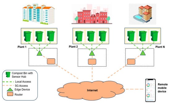
Figure 1.
Compost Monitoring System (CMS) deployment scenario.
3.1. Sensor Hub and Its Installation
The Arduino Uno (R3) is the heart of the sensor hub, serving as the microcontroller that controls the functionality of the compost monitoring system. This controller coordinates the operation of sensors, processes data and communicates with external devices. Each of the sensors is connected to the controller using the interface as listed in Table 1. All these sensors are integrated in a single Printed Circuit Board (PCB). The controller transmits the sensor data via a Universal Asynchronous Receiver-Transmitter (UART) port to the edge device using a Radio Frequency (RF) module Xbee RFX240 (NSK Electronics, Bengaluru, India). The Xbee RFX240 is a physical layer device. In order to keep the system simple and low cost, the RFX240 modules have been used. The range of 100 m supported by Xbee is ideal for the topology considered in campuses. The system range can be improved by using LoRa modules for large-distance applications. Raspberry Pi 3 Model B is used as an edge device and is programmed using the Geany text editor in Python (version: 3.13.0) to receive data from an RF module. The communication port towards the sensor hub is via a UART link of the Raspberry Pi and the Xbee RFX240 radio frequency physical layer device. Both the transmitting and receiving Xbees are set up to communicate with each other at a default speed of 9600 baud rate.

Table 1.
Sensors, descriptions and their interface to controller.
Figure 2 shows the assembled sensor hub. Figure 3 shows the mounting mechanism of the sensor hub into the bin. The diagram shows a schematic representation of the compost bin placed on a metal stand. It features a closing lid at the top and an openable door at the bottom for collecting matured compost. Additionally, the bin is equipped with an outlet valve to collect liquid fertilizer produced during the composting process, which can be used for plants. The sensor hub consisting of an IoT sensor board, controller, RF device and portable battery is attached upside down to a PVC pipe using a clip. The PVC pipe is supported by a stability disk, and the entire system is inserted into the compost bin. Three sensors, namely the compost temperature, soil moisture and pH, are placed dipped inside the compost.
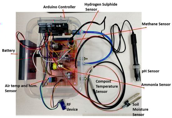
Figure 2.
Assembled sensor hub with controller, sensors and battery.
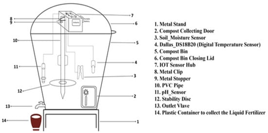
Figure 3.
Illustration of the mechanical design.
The flow of the code in the controller is triggered by the interrupt from the timer set in the RTC. The initialization process involves importing of the libraries for the DHT sensor and the Dallas temperature sensor to measure ambient temperature, relative humidity and compost temperature. It then defines the input pin numbers for the digital sensors. Next, it creates objects for the sensors, allowing the program to communicate with them. Analog pins are assigned for the analog sensors. The variables for the required sensors are defined. The code then initializes serial communication so that data can be printed to the serial monitor and sets the pin modes for the sensors. Once the setup is complete, the code repeatedly reads data from each sensor. This sensor data is continuously collected and transmitted to an RF transceiver for wireless communication after each reading. The loop repeats this process continuously for a set number of time, and then the controller goes into sleep mode.
3.2. Sensor Calibration and Coding
Gas sensors need to be calibrated individually using known concentration levels of the corresponding gases in the air. Gas sensors are calibrated using the sensitivity characteristics graph provided in the datasheet [], which plots gas concentration in parts per million (ppm) against the resistance ratio of the sensor. Here, the resistance ratio is expressed as Rs/R0.
Here, Rs is the sensor resistance in the target gas, and R0 is its resistance in fresh air, obtained by averaging analog readings in fresh air and applying the Rs formula. While the actual relationship between gas concentration and the resistance ratio is exponential, the datasheet uses a logarithmic scale. Hence, a logarithmic straight-line equation is applied as in (1).
Equation (1) is used to determine the slope m and intercept b for calibration.
All MQ sensors need to be preheated by connecting them to a power supply before using them to ensure accurate and stable readings. Typically, the preheating duration is at least 24 h. The soil moisture sensor is designed in such a way that it shows the highest analog value when there is no moisture and the lowest value when moisture is detected. For example, a value of 970 represents the highest analog value (dry), and 505 represents the lowest analog value (wet). These values converted to a percentage, and reversing the scale, show the correct moisture level. pH sensor with probe: The pH sensor consists of two parts, one is sensor circuit pH 4502c and another one is pH electrode e201—BNC pH Electrode. The analog input of the controller is used to measure the pH value. Digitized voltage values range from 0 to 5 V with a resolution of 1024 steps, corresponding to values from 0 to 1023. The pH range goes from 0 to 14, with 7.0 being neutral. These pH sensors can produce negative voltages for acidic solutions (pH < 7) and positive voltages for basic solutions (pH > 7). The calibration of the sensor should accurately cover the entire spectrum of pH values. For attaining this pH 7 (the center of the pH scale) to exactly the middle of the voltage range, the pH electrode is placed in a buffer solution with a pH of 7.0. To calibrate the sensor, the potentiometer is adjusted until the voltage reads half of the reference voltage for pH 7. Averaging of multiple readings is performed to reduce the impact of any sudden spikes or noise in the sensor reading, leading to accurate pH measurements. Ten readings are taken and sorted in the order of magnitude. The extreme values (top two and bottom two) are discarded and the middle six values are averaged before converting to a voltage. It then calculates the pH value, applying a small offset for fine-tuning. By averaging multiple readings and applying an offset, the sensor can be calibrated more effectively, especially if the environment introduces noise.
3.3. Edge and AWS Application
The flow of process in the edge Raspberry Pi begins by initializing necessary variables and importing relevant libraries required for serial communication, handling Java Script Object Notation (JSON) and AWS IoT SiteWise integration []. Then, a file is created using the current date and time to store sensor data in JSON format. The time duration for which the data collection should run is set, and the program attempts to establish a serial connection with the RF device. If the connection fails, the program prints an error message and exits. Once the serial connection is established successfully, the program collects sensor data for the specified duration and stores it in a JSON file. After data collection ends, the program closes the serial connection and extracts numeric values from the raw sensor strings, which are stored in the JSON file. It calculates the average values for each parameter, stores them and prints the results to the local console. The collected parameters are then mapped to AWS IoT SiteWise aliases, and if a parameter is missing, a warning is printed; otherwise, the data is prepared for transmission.
Before sending data to AWS IoT SiteWise, the program verifies AWS credentials. If credentials are missing or incomplete, an error is printed and the process terminates. If the credentials are valid, the data is transmitted to AWS IoT SiteWise and the program ends successfully. This flow ensures efficient data collection and effective error handling. The code flow and AWS integration are given in [].
3.4. Timing Schedule and Battery Life Computations (Refer to Figure 4)
A burst of data from each sensor is collected for a duration of TNS. NB is number of bursts, Ns is number of sensor readings in a burst, TA is the awake time, Ts is the sleep time, TSA is the time period of awake–sleep cycle, TB is the time between bursts, TNS is time period for sending NS sensor readings, N is the number of measurements in a day. IA = average active current in mA,
IS is the sleep current in mA, C is the battery capacity in mAh and battery life in days is given by B in (3)
Number of devices without collision is given by (4).
E.g.: TA = 20 min… 200 bursts, each burst 7 sensors 8 readings, 72 bins can be accommodated. With C = 10,000 mAH, N = 1, B is 10,000/(420) approximately, that is, 23.6 h. Operation of 20 min per day implies 72 days of battery life, which suffices, as the composting cycle time for the compost bins is 45–60 days. IA = 377 mA (sensor card) + 40 mA (controller board), Is = 31 μA.
3.5. Thermal Imaging
Figure 5 shows the composting bin used for thermal imaging experiments. It has a capacity of 800 kg, with dimensions (inch) 40″ H × 35″ B × 35″ W. The material used is UV stabilized, roto-molded plastic. It is meant for outdoor spaces where there is good ventilation. Two vertical and thirteen horizontal vents are present towards this.
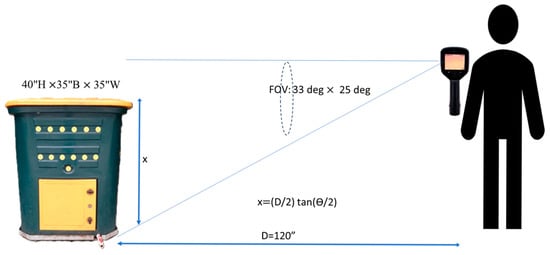
Figure 5.
Bin used for aerobic composting and measurement distance from the thermal camera.
Thermal Camera FLIR E8 Pro is a handheld thermal camera with a higher resolution of 320 × 240 pixels that is capable of capturing detailed thermal images. Thermal imaging calibration has been performed by the vendor in the premises, as per the user manual [].
For image acquisition, the emissivity has been set to 0.95 as part of the calibration process. Other parameters values set are as follows. Reflected temperature set to 20 °C, atmospheric temperature set to 20 °C, relative humidity set to 50% and a fixed measurement distance of 1 m. This procedure is to minimize variability and ensure measurement accuracy []. The camera has a temperature range of −20 °C to 250 °C, which is sufficient for covering the typical temperature range of compost. Regarding the cost implications, the FLIR E8 Pro (320 × 240 resolution) used in this study is priced at approximately INR 323,000, whereas lower-resolution alternatives such as the MLX90640 (32 × 24 resolution) are available for around INR 8500, highlighting the significant trade-off between cost and image quality.
Accuracy of this camera is ±2 °C for ambient temperature 10 °C to 35 °C and object temperature above 0 °C. The Field of View (FOV) is 33° × 25°. The FOV describes the surface visible with a thermal camera, and it depends on the lens used.
Thermal imaging cameras do not allow us to see inside objects but can only be used to identify their surface temperature. The thermal camera measures the IR radiation emitted by objects within its visual field. The calibration process involves the correction of emissivity adjustment depending on the material. The emissivity is especially important when the temperature differences between the measured object and the measurement environment are large []. FLIR provides an auto calibration process. The materials and elements below the surface influence the temperature distribution at the surface of the measurement object. It is often possible to identify the internal structures of the measurement object on the thermal image. However, it is therefore not possible to draw precise conclusions about the temperature values of the elements inside the measurement object.
The smallest detectable object is the smallest dimension that can be identified by a pixel. A pixel is an element on the thermal camera’s detector that records IR rays and converts them into electrical signals. Each pixel corresponds to a measurement value. For an object to be identified from a distance D from the camera, it needs to be of minimum dimension x given by (5) along the horizontal axis (refer to Figure 5).
θ is the FOV along the horizontal axis. Similarly, if y is the minimum dimension of the object along vertical axis, it is related to the φ, the FOV along y axis, as given in (6).
4. Data Analysis and Results
4.1. Sensor Hub-Based Experiments
Two cycles of data with two different bins have been collected. The same sensor hub has been used sequentially for both the bins. The bins used are aerobic ‘hot pile’ decentralized bulk waste composters for apartments, offices, resorts and community institutions. The internal breathing towers regulate air flow and ensure no foul odor. The difference between the two bins has been tabulated in Table 2. Figure 6 shows the pictures of the two bins used.
Table 2.
Comparison of the compost bins used and the measurement conditions.
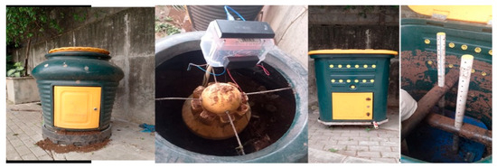
Figure 6.
Two types of bins used for the experiments with top views.
The composting process followed includes two ingredients used with the raw materials. Cocopeat powder is used to adjust the moisture content of raw materials. If the raw material is too wet, it can lead to fungal growth, preventing microbes from effectively decomposing it. The quantity of cocopeat required depends on the moisture level of the raw material []. It is primarily used to maintain an optimal dryness level for proper decomposition []. Compost microbe powder is used to introduce microbes that facilitate the decomposition process. Half a spoon of compost powder is added per 25 kg of raw material used in the process.
The data capture has been started after the bin was full. Bin 1 took 4–5 days to fill while Bin 2 took 2 days to fill up. The composting thus would have started earlier than day 1 of the measurement. The capture schedule has been set for N = 200 samples, approximately 20 min. Interpolation has been applied for missing data. Cycle 1 had 3 days of missing data out of 44 days. Cycle 2 had 8 days of missing data towards the end of the cycle. Figure 7 shows the plot of the temperature of the compost versus the age of the compost.
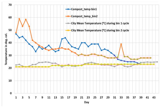
Figure 7.
Compost temperature and city mean temperature versus age of compost.
The mean city temperature was observed to be more or less the same around 21 °C. This has been included in Figure 7 for reference. The general trend observed is that there is a decrease in the temperature as the compost matures. Stability of the temperature is seen from day 33 for bin 1 and day 21 for bin 2. Faster microbe activity is seen for bin 2 because of the difference in the aeration levels, with bin 2 having much better aeration. Figure 8 shows the compost moisture levels. Bin 2 shows lower moisture levels. This could be attributed to the raw materials difference and also the difference in the air relative humidity. Cycle 2 had lower relative humidity values of air, as seen in the plot of Figure 9. pH values measured in the compost are plotted in Figure 10. The pH values as observed on the trendline is between 5 and 8 for cycle 1 and between 4 to 6 for cycle 2. The compost is acidic at the end of the cycles for both the bins. As organic matter decomposes, microorganisms break it down into simpler compounds producing acids, causing a drop in pH value.
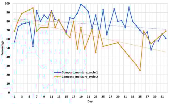
Figure 8.
Compost moisture level.
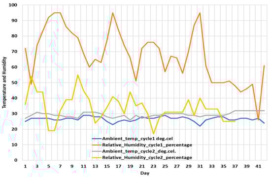
Figure 9.
Ambient temperature and relative humidity of air versus age of compost.
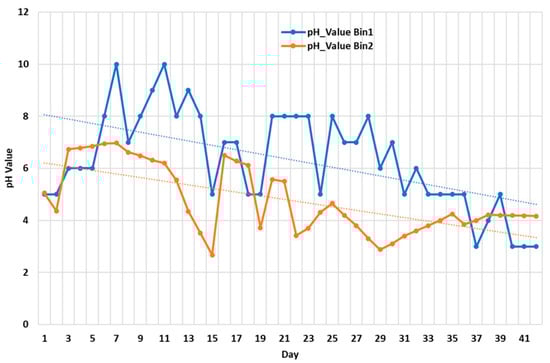
Figure 10.
pH values of compost versus age of compost.
Figure 11 shows the measured increase in the gas levels as compared to the values measured in free air of a room. This gives the relative increase or decrease in gas levels as compared to the room levels. It has been observed that the gas levels are much lower during cycle 1. The gases released during cycle 2 are relatively higher. This could indicate the anaerobic conditions during the cycle. Figure 12 shows the absolute measured values along with the threshold levels of ammonia and methane, beyond which it is dangerous. The level of hydrogen sulfide needs to be zero or minimal. It is to be noted that the ammonia and methane are very much lower the threshold values.
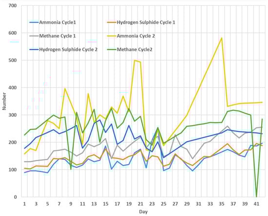
Figure 11.
The relative gas levels with respect to room levels versus age of compost.
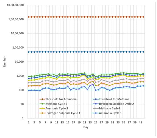
Figure 12.
Gas levels with respect to danger level threshold.
Figure 13 and Figure 14 show the correlation between the various parameters measured. A few obvious inferences that can be drawn are:
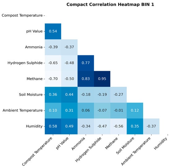
Figure 13.
The correlation between parameters for bin 1.
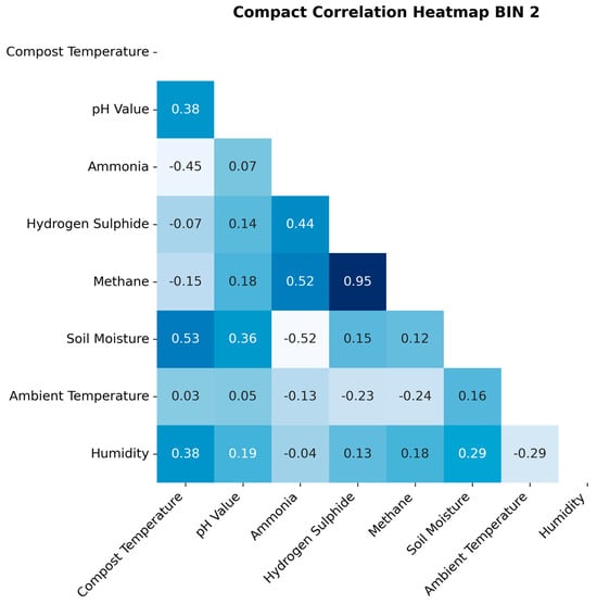
Figure 14.
The correlation between parameters for bin 2.
Common observations across both bins are that (i) hydrogen sulfide and methane are highly correlated to each other. (ii) Ammonia generated is related to methane and hydrogen sulfide generated. (iii) Moisture in compost is related to compost temperature and pH value. (iv) Compost temperature is related to air humidity. pH value and compost temperature are related to each other. (v) Ammonia generated is related inversely to compost temperature.
4.2. Thermal Camera-Based Experiments
The FLIR E8 Pro camera has been used to collect the day-wise thermal data. Measurements were taken daily between 2 and 3 p.m., along with the temperature probe measurements, for a cycle of composting between 22 April 2025 and 2 June 2025. The thermal images have been cropped using Galaxy photo-assist in order to remove the background. Then, the RGB image has been converted to gray scale. The data was processed using R programming (version 4.5.0) to create grayscale images, generate histograms and find the mean and variance of the images. The R packages used for the image processing are magick, showimage and imager []. Figure 15 shows the details of the processing involved. The results obtained from the gray-scale image processing are explained in this section.
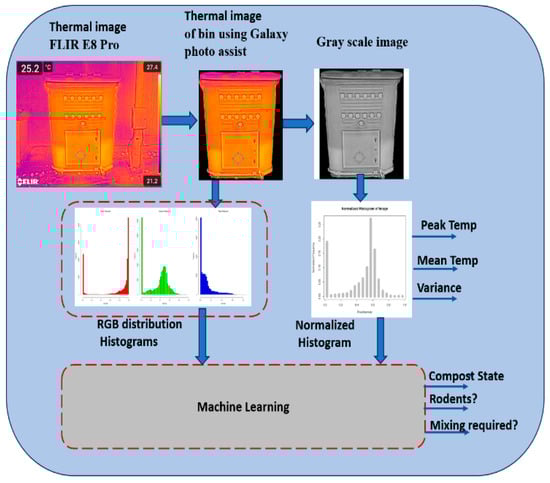
Figure 15.
Processing of the captured images.
An image can be represented by a rectangular matrix of discretized data (pixels). Each pixel can be notated by p[q, r], where the indices (q, r) are integers, with q = 0, 1 … Q − 1, r = 0, 1 … R − 1. Each pixel value p takes a value from the range 0 to 255. Pixel intensity is the normalized pixel value range from 0 to 1, i.e., p/256. The total number of pixels is Q × R. nl is the number of pixels of each gray level bin (frequency). The normalized frequency value at each gray level is given by (7).
L is the number of gray-level bins of the histogram. Pl represents the probability. Mean intensity is given by (8), summation of the product of intensity values and probabilities.
The variance obtained from the histogram is given by (8). Variance of the intensity is given by (9).
4.2.1. Observation 1
Day-wise temperature measurement using probe and maximum temperature measured by the thermal camera is shown in Figure 16. It can be observed that there is a difference between the sensor probe measurement and the measurement made by the thermal camera till day 21, after which both the readings converge to the ambient temperature. It needs to be noted that the probe samples the temperature by its resistive sensor, at the spot of insertion, about a half foot depth near the center of the bin. The thermal camera gives the surface temperature profile, and the maximum temperature is the measurement noted. This maximum temperature could be at any spot within the bin. The surface temperature measurements are definitely lower than that of the actual inside temperature. The compost material, bin material and thickness and the outside air conditions determine the surface temperature. A thermal camera measures long wavelength infrared radiation emitted by an object, and the intensity of the infrared radiation emitted depends on the surface emissivity of the material. Accurate adjustment of the emissivity is important, especially when the temperature differences between the measured object and the measurement environment are large [].
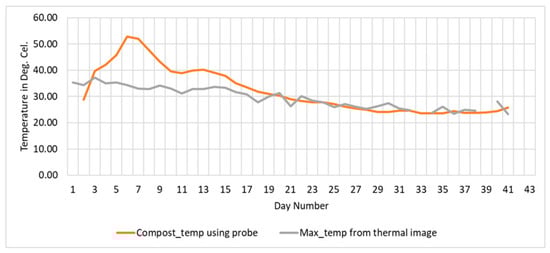
Figure 16.
Day-wise temperature measurements using probe and maximum temperature given by camera.
The weather conditions also make a difference to the readings []. The ideal conditions for outdoor infrared measurements are on cloudy days, because the measuring object is protected against radiations. Measurement errors are caused if the bin is moist because the surface of the measured object is cooler. Fogging of the thermal camera lens happens in humid or cold weather, and not all of the infrared radiation can be received []. During rain, the water droplets in the transmission line allow lesser infrared rays to pass. The heat exchange effect increases as a function of the temperature difference between the surface of the measurement object and the ambient temperature. Direct sun light can emit infrared thermal radiation and can therefore influence the temperature of objects in their environment.
4.2.2. Observation 2
The variance plot of the histogram converges as shown in Figure 17 to a low value, indicating that all the pixels have reached a particular value. The histograms during composting have higher variance, implying widespread values of temperature distributed spatially in the bin.
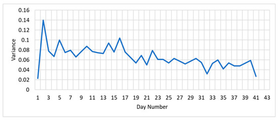
Figure 17.
Day-wise variance of the temperature measurement obtained from gray-scale histogram.
The usage of these observations can be to detect the state of composting, presence of rodents, identification of anaerobic pockets, or requirement of mixing [,]. A uniform temperature should be maintained throughout the compost bin to prevent localized pockets of anerobic activity. Figure 18 shows the histogram with the thermal image of day 1, day 15 and day 40. The differences in the distribution are because of the changes in the compost as well as the weather impact.
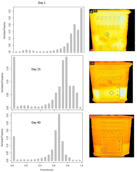
Figure 18.
Day 1, day 15, day 40 histogram and thermal images.
The thermal imaging experiments are being performed as a part of proving a contactless method of detecting the compost status. Rather than the absolute value, the trend or slope of the temperature variation can define the events of the compost life cycle.
The prototype is useful to optimize the number of sensors required. For example, the high correlation between the H2S and methane suggests that one of these can be removed from the system to save on cost and power. The alerts that can be generated during the operations phase are listed in Table 3. It can be seen that the developed system can be used for research of the composting process. For example, there are observations that pH value is related to air humidity in cycle 1 bin 1 only. Methane generated is related to air humidity in cycle 1 only. pH value and ammonia are related in bin 1 only. The pH, compost temp and hydrogen sulfide are related in bin 1 only. These observations, listed in Table 4, can be investigated further. Further work on using a recommendation system to provide feedback with corrective actions possible, based on the measurements and alerts generated, will enhance the usage tremendously.
Table 3.
Alerts and their description.
Table 4.
Relations unique to BIN 1 and BIN 2.
5. Conclusions
The design details required for the development of a compost monitoring system have been presented. The deployment scenario of the bins in residential communities has been considered for the functional testing of the prototypes. The data collected over multiple cycles has been analyzed, and their plots have been shown as a part of the results.
This paper has also discussed a contactless method of monitoring the compost using thermal imaging. Thermal images for an entire cycle of an aerobic compost bin of the campus have been collected and analyzed. The processing involved in the analysis has been described. The observations on how these results differ from the temperature probe measurements have been discussed. Analysis of the spatial information obtained by thermal imaging for understanding the composting process has been discussed, bringing out its advantages in generating alerts for mixing action.
The thermal imaging experiments were conducted to check on the feasibility of contactless monitoring and checking on rodents. A tiltable wall-mounted camera which spans the compost bins is the long-term plan. It can be used to augment or replace the functionality of finding the compost readiness, though not the odor information.
The cost of the thermal camera is one major bottleneck to widespread usage. To address this issue, a low-cost thermal camera with 32 × 24-pixel resolution is being looked into, which can give similar results. Usage of RGB channels can enhance the insights, and this needs to be looked into.
The current experimental prototype uses only two bins; this limited scope has been chosen to validate the basic functionality of the prototype. Large-scale behavior, though theoretically validated, needs to be tested. The primary scalability bottleneck is the probability of packet collisions, which can be avoided by using number of bins less than M indicated in (4).
The use of solar power for the system, study of transmission rate and power consumed, etc., to increase the life span of battery can be further investigated.
The system, being a prototype for functional study, has not been subjected to environmental tests. It had been operational in temperatures between 10 °C and 40 °C approximately during the experiments. The next model needs to take the environmental testing into consideration.
Author Contributions
Conceptualization, methodology, writing—original draft preparation, S.G.V.K.; software, validation, A.B.; formal analysis, writing—review and editing, C.S.K.; visualization, writing—review, project administration, funding acquisition, J.B. All authors have read and agreed to the published version of the manuscript.
Funding
This research was funded by IIITB COMET Foundation 0001.
Data Availability Statement
Data is provided in the GitHub link: https://github.com/Siva-K67/Compost-Monitoring-System (accessed on 20 September 2025).
Conflicts of Interest
The authors declare no conflict of interest.
Abbreviations
The following abbreviations are used in this manuscript:
| AWS | Amazon Web Services |
| IoT | Internet of Things |
| JSON | Java Script Object Notation |
| PCB | Printed Circuit Board |
| RF | Radio Frequency |
| UART | Universal Asynchronous Receive Transmit |
| FoV | Field of Vision |
References
- Maria Mercede Martinez, M.M. Farmer’s Compost Handbook; FAO—Food and Agriculture Organization of the United Nations: Rome, Italy, 2015; ISBN 978-92-5-107845-7. [Google Scholar]
- Quan, J.; Wang, Y.; Wang, Y.; Li, C.; Yuan, Z. An efficient strategy to promote food waste composting by adding black soldier fly (Hermetia illucens) larvae during the compost maturation phase. Resour. Environ. Sustain. 2024, 18, 100180. [Google Scholar] [CrossRef]
- Daily Dump. Available online: www.dailydump.org (accessed on 1 August 2025).
- Turvani, G.; Fiore, M.; Rodriguez-Duarte, D.O.; Demichelis, F.; Tommasi, T.; Vipiana, F.; Riente, F. Enabling High-Quality Compost for a Smart Domestic Production. In Proceedings of the IEEE International Workshop on Metrology for Agriculture and Forestry (MetroAgriFor), Pisa, Italy, 6–8 November 2023; pp. 837–841. [Google Scholar] [CrossRef]
- Wardhany, V.A.; Hidayat, A.; A., M.D.S.; Subono; Afandi, A. Smart Chopper and Monitoring System for Composting Garbage. In Proceedings of the 2nd International Conference of Computer and Informatics Engineering (IC2IE), Banyuwangi, Indonesia, 10–11 September 2019; pp. 74–78. [Google Scholar] [CrossRef]
- Hemidat, S.; Jaar, M.; Nassour, A.; Nelles, M. Monitoring of Composting Process Parameters: A Case Study in Jordan. Waste Biomass Valoriz. 2018, 9, 2257–2274. [Google Scholar] [CrossRef]
- Shalini, V.B.; Maheswari, A.U.; Marimuthu, C.; Jeshima, J. Vermi-Composting using AI in IoT. In Proceedings of the International Conference on Applied Artificial Intelligence and Computing (ICAAIC), Salem, India, 9–11 May 2022; pp. 1489–1493. [Google Scholar] [CrossRef]
- Elalami, M.; Baskoun, Y.; Beraich, F.Z.; Arouch, M.; Taouzari, M.; Qanadli, S.D. Design and Test of the Smart Composter Controlled by Sensors. In Proceedings of the 7th International Renewable and Sustainable Energy Conference (IRSEC), Agadir, Morocco, 27–30 November 2019; pp. 1–6. [Google Scholar] [CrossRef]
- Nikoloudakis, Y.; Panagiotakis, S.; Manios, T.; Markakis, E.; Pallis, E. Composting as a Service: A Real-World IoT Implementation. Future Internet 2018, 10, 107. [Google Scholar] [CrossRef]
- Jo, R.S.; Lu, M.; Raman, V.; Then, P.H.H. Design and Implementation of IoT-Enabled Compost Monitoring System. In Proceedings of the IEEE 9th Symposium on Computer Applications & Industrial Electronics (ISCAIE), Kota Kinabalu, Malaysia, 27–28 April 2019; pp. 23–28. [Google Scholar] [CrossRef]
- Morehead, B.; Morehead, J.M.; Morehead, J.T.; Morehead, T.R.; Morehead, L.E. Smart Composting Apparatus. U.S. Patent Application US2021/0355045A1, 18 November 2021. [Google Scholar]
- Bhoir, R.; Thakur, R.; Tambe, P.; Borase, R.; Pawar, S. Design and Implementation of Smart Compost System Using IoT. In Proceedings of the IEEE International Conference for Innovation in Technology (INOCON), Bengaluru, India, 6–8 November 2020; pp. 1–5. [Google Scholar] [CrossRef]
- Pearl, Y.; Pearl, Y.; Pearl, Z. System and Method for Composting. Patent WO2021/183797, 16 September 2021. [Google Scholar]
- Tomicic, J. IoT-Based Agricultural Compost Monitoring System: Prototype Development and Sensor Technology Evaluation. Compost Sci. Util. 2023, 30, 1–14. [Google Scholar] [CrossRef]
- Bhardwaj, S.; Singh, A.K.; Tripathi, U.; Ujjawal, S.; Goel, S.; Kumar, A. An IoT-Based Approach to Measure the Effectiveness of Traditionally Prepared Compost in Indian Villages. In Proceedings of the 2024 International Conference on Computing, Sciences and Communications (ICCSC), Ghaziabad, India, 24–25 October 2024; pp. 1–7. [Google Scholar] [CrossRef]
- Yun, H.; Lo, S.; Diepenbrock, C.H.; Bailey, B.N.; Earles, J.M. VisTA-SR: Improving the Accuracy and Resolution of Low-Cost Thermal Imaging Cameras for Agriculture. In Proceedings of the IEEE/CVF Conference on Computer Vision and Pattern Recognition Workshops (CVPRW), Seattle, WA, USA, 17–21 June 2024; pp. 5470–5479. [Google Scholar] [CrossRef]
- Jaycon Systems. Understanding a Gas Sensor; Jaycon Systems: Orlando, FL, USA, 28 September 2023; Available online: https://www.jaycon.com/understanding-a-gas-sensor/ (accessed on 5 August 2025).
- AWS IoT SiteWise Documentation. Available online: https://docs.aws.amazon.com/iot-sitewise/ (accessed on 14 April 2025).
- Siva-K67. Compost-Monitoring-System. GitHub. 2025. Available online: https://github.com/Siva-K67/Compost-Monitoring-System (accessed on 20 September 2025).
- Wilson, N.; Gupta, K.A.; Koduru, B.H.; Kumar, A.; Jha, A.; Cenkeramaddi, L.R. Recent Advances in Thermal Imaging and Its Applications Using Machine Learning: A Review. IEEE Sens. J. 2023, 23, 3395–3407. [Google Scholar] [CrossRef]
- Boldrin, A.; Andersen, J.K.; Møller, J.; Christensen, T.H.; Favoino, E. Composting and Compost Utilization: Accounting of Greenhouse Gases and Global Warming Contributions. Waste Manag. Res. 2009, 27, 800–812. [Google Scholar] [CrossRef]
- Xiong, Z.-Q.; Wang, G.-X.; Huo, Z.-C.; Yan, L.; Gao, Y.-M.; Wang, Y.-J.; Gu, J.-D.; Wang, W.-D. Effect of Aeration Rates on the Composting Process and Loss of Nitrogen during Composting. Appl. Environ. Biotechnol. 2015, 2, 20–28. [Google Scholar] [CrossRef]
- Bektaş, D.; Girgin, M.; Akgül, T. The Effect of Surface Temperature on Infrared Reflections in a Thermal Image. In Proceedings of the 2024 32nd Signal Processing and Communications Applications Conference (SIU), Mersin, Türkiye, 15–18 May 2024; pp. 1–4. [Google Scholar] [CrossRef]
- Aburto Medina, A.; Shahsavari, E.; Khudur, L.; Brown, S.; Ball, A. A Review of Dry Sanitation Systems. Sustainability 2020, 12, 5812. [Google Scholar] [CrossRef]
- Cai, S.; Ma, Y.; Bao, Z.; Yang, Z.; Niu, X.; Meng, Q.; Qin, D.; Wang, Y.; Wan, J.; Guo, X. The Impacts of the C/N Ratio on Hydrogen Sulfide Emission and Microbial Community Characteristics during Chicken Manure Composting with Wheat Straw. Agriculture 2024, 14, 948. [Google Scholar] [CrossRef]

Disclaimer/Publisher’s Note: The statements, opinions and data contained in all publications are solely those of the individual author(s) and contributor(s) and not of MDPI and/or the editor(s). MDPI and/or the editor(s) disclaim responsibility for any injury to people or property resulting from any ideas, methods, instructions or products referred to in the content. |
© 2025 by the authors. Licensee MDPI, Basel, Switzerland. This article is an open access article distributed under the terms and conditions of the Creative Commons Attribution (CC BY) license (https://creativecommons.org/licenses/by/4.0/).