Mapping Olive Crops (Olea europaea L.) in the Atacama Desert (Peru): An Integration of UAV-Satellite Multispectral Images and Ensemble Machine Learning Models

Abstract

Spatial monitoring of olive systems in arid regions is essential for understanding agricultural expansion, water pressure, and productive sustainability. This study aimed to map coverage and estimate olive plantation density (Olea europaea L.) in the Atacama Desert, Tacna (Peru) through the integration of UAV-satellite multispectral images and machine learning algorithms (CART, Random Forest, and Gradient Tree Boosting). Forty-eight optical, radar, and topographic covariates were analyzed. Fifteen were selected for coverage classification and 16 for plantation density, using Pearson’s correlation (|r| > 0.75). The classification maps reported an area of 23,059.87 ha (38.21%) of olive groves, followed by 5352.10 ha (8.87%) of oregano cultivation and 725.74 ha (1.20%) of orange cultivation, with respect to the total study area, with overall accuracy (OA) of 86.6% and a Kappa coefficient of 0.81. Meanwhile, the RF and GTB regression models showed R² ≈ 0.89 and RPD > 2.8, demonstrating excellent predictive performance for estimating tree density (between 1 and 8 trees per 100 m²). Furthermore, the highest concentration of olive trees was found in the central and southern zones of the study area, associated with favorable soil and microclimatic conditions. This work constitutes the first comprehensive approach for olive mapping in southern Peru using UAV–satellite fusion, demonstrating the capability of ensemble models to improve agricultural mapping accuracy and support water and productive management in arid ecosystems.

1. Introduction

The olive tree (Olea europaea L.) is considered one of the oldest and most important fruit trees, cultivated in more than 50 countries [1,2]. Fruit production and olive oil represent a traditional and widespread activity in the highly relevant agri-food sector in the Mediterranean region, responsible for more than 95% of world olive production [1,3]. The European Union is one of the world’s largest producers, consumers, and exporters of olive oil. Spain, Italy, and Greece represent approximately 66% of world production [4]. Current trends report an increase in agricultural areas of olive cultivation centered in South America, Argentina, and Australia [1,5]. This increase in areas is associated with inadequate agroecological practices in agricultural management (use of pesticides, herbicides, chemical fertilizers, inadequate irrigation, and waste management) that can generate environmental impacts such as soil erosion and significant decrease in fertility [6,7,8]. Furthermore, olive trees suffer the effects of droughts and high temperatures causing greater evaporation demand and lower water availability in the soil, especially under rainfed conditions, putting the olive sector at risk [9].

In Chile and southern Peru, we find the Atacama Desert characterized by arid and saline zones with important agro-industrial potential where olive crops predominate [10,11]. In Peru, more than 28,000 ha have been reported for the production of olives (75%) and olive oil (25%) destined for national and international consumption [12,13]. However, climate change and overexploitation of water resources are affecting the efficiency of olive production and the quality of its products [10,14]. Spatially evaluating olive plantations could provide accurate information about the extent of crops, assess the impacts of olive intensification on water resources, and improve their management [3,15]. In this sense, the application of remote sensing could facilitate large-scale crop mapping and analyze some physiological traits of the crop [2,16,17,18,19,20,21,22,23,24].

Remote sensing emerges as an indispensable tool widely used in precision agriculture for the management and monitoring of sustainable agriculture [25]. A robust tool for plantation monitoring, including mapping, detection of soil cover changes, plant counting, pest or disease detection, yield estimation [19,26,27,28,29,30]. The detection and counting of olive trees based on high-resolution images, whether satellite or obtained through Unmanned Aerial Vehicles (UAV), is important because it can provide accurate information to generate biomass estimation models, carbon stock calculation, yield prediction [31,32,33,34]. Likewise, to provide information on the distribution, growth, and production of plantations, which will help in plantation management, irrigation, and resource use [19,35,36].

In recent years, with the increase in accessibility to remote sensing data, the advancement of spatial analysis algorithms, and the development of cloud processing platforms, the number of studies focused on olive crop mapping has increased significantly. These approaches can be grouped into three main categories: (1) traditional methods based on image processing, which employ techniques such as segmentation, binarization, or local maximum filtering [37,38,39]; (2) methods based on machine learning, which integrate algorithms such as support vector machines (SVM), random forests (RF), Classification and Regression Tree (CART), Gradient boosting (XGBoost), or artificial neural networks (ANN), combined with spectral and textural feature extraction processes [3,27,40,41,42]; and (3) methods based on deep learning, which use convolutional neural networks (CNN) and advanced architectures for crown detection and segmentation from UAV and satellite multispectral images [19,26,27].

The department of Tacna (Peru), considered the first national olive producer [13]. However, in recent years the crop has been affected by pests and diseases that reduce crop production [43]. Added to this, the limited availability of spatial information on its spatial distribution and the number of plantations, which limits management and the implementation of pest and disease control and mitigation actions. Therefore, it is proposed to apply a pixel-level mapping approach of olive plantations to differentiate tree species (orange, oregano and other crops) using UAV-satellite images to generate olive distribution maps for the entire Atacama Desert of Tacna in Peru. The objectives were (i) to map the coverage and estimate the density of olive trees by integrating UAVs, satellite images (Sentinel-1 and Sentinel-2), and topographic variables; (ii) to integrate optical indices, radar texture metrics, and topographic variables to determine the most important variables for mapping and estimating olive tree density; and (iii) to determine ensemble models (RF, CART, and GTB) for both classification and density regression.

2. Materials and Methods

2.1. Study Area

The study area is in the province and department of Tacna, Peru in the northern zone of the Atacama Desert between the border with Chile (Figure 1a,b). The study area is characterized by having an arid and temperate climate with moisture deficiency in all seasons of the year [43,44]. According to the La Yarada meteorological station, the maximum temperature ranges between 20.0 and 28.2 °C between the months of December to March, while the minimum temperature ranges between 12.7 and 18 °C in the months of July to August (Figure 1c). Meanwhile, the average annual precipitation is 4.2 mm, with the months of July to September having the highest precipitation [44].

Figure 1. The study area covers the Atacama Desert of Peru in the province of Tacna in the department of Tacna, (a) study area, La Yarada irrigation district, Tacna department, Peru, (b) location of the study area in Peru and South America, and (c) climograph of the La Yarada station in the study area.

Land use is characterized by lands with scarce vegetation and lands with fruit trees and permanent crops [45]. The study area is suitable for olive cultivation (approximately 23,168 ha) [13], due to climate and soil characteristics, in addition to other crops such as orange, mandarin, grapevine, oregano, and alfalfa [45]. The availability in the study area for human consumption and agriculture is increasingly limited, with the Caplina aquifer as the main source [46]. According to the MapBiomas 2024 map, vegetation cover and land use are characterized by dry forest covers, non-forest formations, areas without vegetation, and agricultural mosaics [47].

Figure 2 shows the methodological workflow developed in three stages: (a) data acquisition, where multispectral images with UAV, spectral signatures, and training areas were obtained, (b) mapping by classification through the integration of satellite images and digital elevation models, and (c) mapping of olive tree density by regression and elaboration of the final olive map.

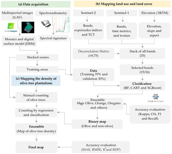
Figure 2. Methodological flowchart for olive crop mapping.

2.2. Data Acquisition

2.2.1. UAV Data and Processing

Multispectral imagery was collected over 14 plots distributed across the study area using an Altum-PT camera (MicaSense, Inc., Seattle, WA, USA) mounted on a DJI Matrice 350 RTK UAV (DJI, Shenzhen, China) (Figure 3a). The system integrates multispectral, panchromatic, and thermal sensors, enabling simultaneous acquisition of high-resolution spectral and thermal data (Figure 3b). The multispectral sensor acquired imagery at 12-bit radiometric resolution in five spectral bands with the following central wavelengths (±bandwidth): blue (475 ± 16 nm), green (560 ± 13.5 nm), red (668 ± 8 nm), red edge (717 ± 6 nm), and near-infrared (842 ± 28.5 nm). Each band was captured at a spatial resolution of 2064 × 1544 pixels (≈3.2 MP per band). Thermal data were acquired in the long-wave infrared (LWIR) region with a resolution of 320 × 256 pixels, allowing the integration of spectral and thermal information for subsequent analysis.

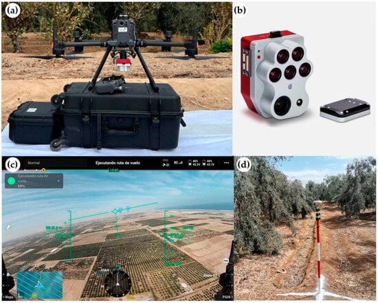
Figure 3. (a) Matrice 350 UAV integrated with the Altum PT sensor, (b) Altum PT camera, (c) Ground control points (GCP), and (d) flight plan for the study image.

Flight campaigns were carried out between 9:00 and 16:00 h during 27, 28, and 29 July 2025, at a height of 150 m above ground level. Images were captured with a 1 s interval and a frontal and lateral overlap of 75% and 80%, respectively (Figure 3c) [48]. In each flight, three ground control points (GCPs) were established, measured with a South G3 Global Navigation Satellite System (GNSS) (horizontal accuracy: 1 cm + 1 ppm RMS; vertical: 2 cm + 1 ppm RMS), to ensure correct alignment and georeferencing of the acquired images (Figure 3d).

Images were preprocessed in .tiff format in Pix4D Pro Mapper (Prilly, Switzerland), incorporating the GCPs to improve geometric and radiometric accuracy. As a result, multispectral orthomosaics were generated that included the thermal band, as well as the digital surface model (DSM) for each plot.

In parallel, reference spectral signatures of olive (Figure 4a,b), orange plantations (Figure 4c) oregano (Figure 4d) and other uses were obtained using a FieldSpec HandHeld FSHH 325–1075P spectroradiometer. These spectral signatures were used as training areas during the satellite image classification process.

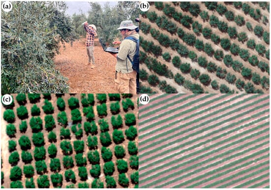
Figure 4. Spectral signature acquisition using (a) spectroradiometer, of (b) olive, (c) orange, and (d) oregano.

2.2.2. Manual Counting of Olive Trees

Counting of each olive and orange tree was performed manually through visual interpretation in the Geographic Information Systems (GIS) interface [49,50]. For this purpose, the mosaics of the plots obtained in Section 2.2.1 were used. This was performed to apply the regression model to obtain the density of olive crop plantations [51] for each 10 × 10 m (100 m²) pixel obtained from the satellite images. A total of 132,864 olive trees and 14,615 orange trees were identified from the multispectral mosaics of the 14 plots (Figure 5).

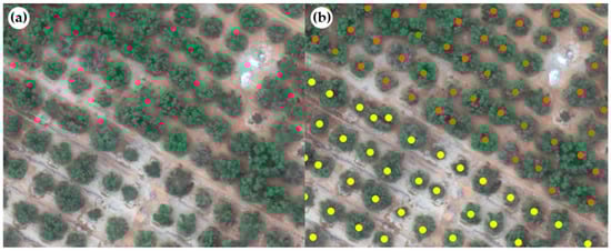
Figure 5. Manual counting through visual interpretation of olive and orange trees (a) UAV RGB combination image and (b) creation of individual points of olive trees (yellow) and orange (orange) on the UAV RGB image.

2.2.3. Training and Validation Areas

At this stage, training areas were collected which were represented by the covers of (i) olive, (ii) oregano, (iii) orange, and (iv) other uses (water bodies, urban area, and bare soil). For this, the olive, orange, and oregano classes were obtained from the mosaics of each flight performed, while the other uses class was obtained from Google Earth and Sentinel-2 images that were implemented on the GEE platform [52].

2.3. Mapping at Satellite Image Level

2.3.1. Integration of Sentinel-2, Sentinel-1 Images and Digital Elevation Models

In GEE, the collections of Sentinel-1 images (ID: COPERNICUS/S1_GRD), Sentinel-2 (ID: COPERNICUS/S2_SR_HARMONIZED), and digital elevation models from the Shuttle Radar Topographic Mission (SRTM) were integrated [53]. This was performed to generate a multiband mosaic from 1 January to 15 August 2025, integrating bands, spectral indices, temporal metrics, texture variables, and variables derived from the digital elevation model. For Sentinel-1 images, temporal statistics were estimated from the polarization bands (VV and VH) median, the 25th and 75th percentile, and the standard deviation. From this, temporal spectral metrics were estimated using texture variables of the Gray Level Co-occurrence Matrix (GLCM) [54,55,56,57]. Likewise, for the median composite of the descending VH series using a moving window of 5 × 5, with a displacement of 1, and averaged in four spatial orientations [58].

We masked clouds and cloud shadows using the scene classification band (SLC) provided in the Level 2A product [30,59] and considering <30% cloudiness. In addition, the mean pixel value per season was used for the analysis for Sentinel-2 images [60]. This allowed calculating spectral indices related to vegetation, soil, and water complemented with the application of Tasseled Cap Transformation (TCT) that generates brightness, greenness, and wetness components, useful for differentiating agricultural covers in heterogeneous landscapes [61]. The layers derived from Sentinel-1, Sentinel-2 images, and topographic variables (elevation, slope, and aspect) were resampled to a 10 m grid using the nearest neighbor approach in GEE [52].

2.3.2. Covariate Selection

It has been shown that a high number of input bands can present multicollinearity and information redundancy, which could affect classifier performance, which can negatively affect crop class detection and classification [62,63,64]. Covariate selection aimed to reduce data dimensionality by eliminating unnecessary features or adding features into a smaller set of non-redundant components [60,65]. We reduced the multicollinearity of the variables by calculating the decorrelation matrix of all variables and removing all features above 0.75, using the same threshold proposed by Jin et al. [66]. Figure 6 shows the decorrelation of the 48 variables obtained for olive crop classification.

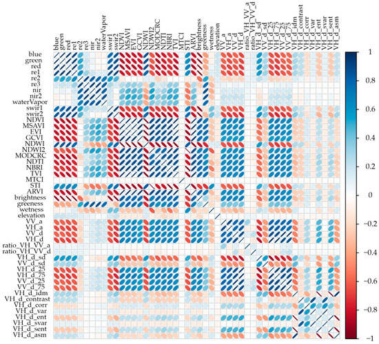
Figure 6. Decorrelation matrix of the 48 variables for olive crop classification.

2.3.3. Olive Crop Classification

From the selected covariates and training areas obtained in previous steps, we applied three pixel-level classification methods due to the high heterogeneity of the study area. Areas were randomly divided into 70% for training and 30% for validation to generate the crop map [58]. We applied logic-based machine learning regression methods to map cover and land use, such as CART, RF, and XGBoost in GEE. We applied logic-based machine learning regression methods to map land cover and land use, such as CART, RF, and XGBoost in GEE. This was because (i) CART was used as the base model due to its interpretability and because it is the fundamental structure from which RF and GTB are built; (ii) RF was selected for its ability to handle high-dimensional datasets, its robustness to noise and multicollinearity, and its good performance reported in agricultural mapping studies; and (iii) GTB was chosen for its ability to capture complex nonlinear relationships through sequential boosting and regularization, which typically translates into high predictive power [48]. These models share a decision tree logic, which facilitates the direct comparison of results and the interpretation of variable importance [67].

CART is a non-parametric algorithm based on successive binary splits that separate data according to optimal thresholds to minimize error or impurity [68]. It allows modeling non-linear relationships and handling outliers or missing values without distribution assumptions [48]. Although flexible, it presents high sensitivity to small variations in data, so it is used as a base model in more complex methods such as RF and XGBoost [69]. RF is an algorithm that combines multiple decision trees trained on random data subsets using bagging [70]. This approach reduces variance and improves model stability compared to a single tree. RF efficiently handles continuous and categorical variables, without requiring normality assumptions, and is robust against overfitting.

The two main parameters of RF are ntree (number of trees growing in the forest) and mtry (number of variables used in each tree) [71]. The out-of-bag error was used to determine mtry and ntree [72]. XGBoost extends traditional gradient boosting by incorporating regularization and sequential optimization [73]. Each new tree corrects the residual errors of the previous one, reducing overfitting and improving generalization. The main parameters of XGBoost include learning rate, max_depth, max_delta_step, subsample [72]. Its stochastic and efficient structure allows precise integration of optical and radar variables.

We used 1000 trees, as initial tests showed no improvements in classification accuracy with a higher number. We applied the CART, RF, and XGBoost tools implemented in GEE for classification [52]. We then applied an ensemble of the three models considering the media for the study area.

2.3.4. Accuracy Evaluation

The accuracy evaluation of the crop classification map was carried out using widely recognized performance metrics: precision, harmonic score (F1-Score), overall accuracy (OA), quantity disagreement (QD), and allocation disagreement (AD). These indices provide complementary perspectives on model performance, allowing both the identification accuracy and the spatial consistency of the classification to be assessed.

$$\mathrm{P}\mathrm{r}\mathrm{e}\mathrm{c}\mathrm{i}\mathrm{s}\mathrm{i}\mathrm{o}\mathrm{n}={\displaystyle \frac{\mathrm{T}\mathrm{P}}{\mathrm{T}\mathrm{P}+\mathrm{F}\mathrm{P}}}\times 100\mathrm{\%}$$

(1)

$$\mathrm{F}1 \mathrm{S}\mathrm{c}\mathrm{o}\mathrm{r}\mathrm{e}=2\times {\displaystyle \frac{\mathrm{p}\mathrm{r}\mathrm{e}\mathrm{c}\mathrm{i}\mathrm{s}\mathrm{i}\mathrm{ó}\mathrm{n}\times \mathrm{r}\mathrm{e}\mathrm{c}\mathrm{a}\mathrm{l}\mathrm{l}}{\mathrm{p}\mathrm{r}\mathrm{e}\mathrm{c}\mathrm{i}\mathrm{s}\mathrm{i}\mathrm{ó}\mathrm{n}+\mathrm{r}\mathrm{e}\mathrm{c}\mathrm{a}\mathrm{l}\mathrm{l}}}\times 100\mathrm{\%}$$

(2)

$$\mathrm{O}\mathrm{A}={\displaystyle \frac{\mathrm{T}\mathrm{P}+\mathrm{T}\mathrm{N}}{\mathrm{T}\mathrm{P}+\mathrm{F}\mathrm{P}+\mathrm{T}\mathrm{N}+\mathrm{F}\mathrm{N}}}$$

(3)

$$\mathrm{Q}\mathrm{D}={\displaystyle \frac{1}{2}} {\sum }_{i=1}^n\left|r_i-c_i\right|$$

(4)

$$\mathrm{A}\mathrm{D}=1-\mathrm{O}\mathrm{A}-\mathrm{Q}\mathrm{D}$$

(5)

where TP, FP, TN, and FN indicate true positive, false positive, true negative, and false negative, respectively. In this study, a true positive refers to a case where both the prediction and the reference label belong to the same class (olive, orange, oregano, or other uses), while a false positive represents cases where a pixel is assigned to one of these classes but the reference indicates a different category. The same logic applies for true and false negatives. Among these metrics, precision and recall quantify the proportion of correctly identified pixels and the proportion of actual class pixels correctly detected; the F1-Score represents their harmonic mean, providing a balanced measure of classification accuracy; and OA reflects the overall proportion of correctly classified pixels. The additional metrics quantity disagreement (QD) and allocation disagreement (AD) decompose the total classification error (1 − OA) into two components: QD measures the difference in the quantity of pixels assigned to each class, while AD measures the spatial disagreement or misallocation between the classified and reference maps [74]. Incorporating these metrics allows for a more comprehensive assessment of classification performance, distinguishing between over- or underestimation of classes and spatial allocation errors, which is particularly relevant in heterogeneous agricultural landscapes such as the Atacama Desert.

2.4. Individual Olive Crop Mapping

2.4.1. Olive Mapping by Regression and Classification

To estimate the spatial density of olive plantations, an approach based on spatial regression was used. First, from the supervised classification thematic map, only the class corresponding to “olive” was extracted, which was used as a base layer for the analysis. Second, a regular mesh of 10 × 10 m cells was generated over the cultivated areas, in which the number of olive individuals per cell was manually counted using UAV images. The centroid of each cell was calculated and associated with the corresponding density value (number of plants per 100 m²), thus forming the set of point observations.

In a complementary manner, the most relevant covariates were extracted derived from optical data (vegetation spectral indices), radar (VH and VV backscatter, and polar ratios), topographic, and texture data for the area occupied by olive groves. Third, a regression model was implemented in RStudio version 2025.09.2+418, using the set of centroids as training and validation data. Furthermore, classification was estimated using the CART, RF, and GTB models for both regression and classification. This procedure allowed modeling the relationship between spectral covariates and tree density, generating a continuous map of spatial distribution of olive crop density. The final result represents the spatial variation in planting intensity (trees/m²) in olive-growing areas.

2.4.2. Model Validation and Accuracy Evaluation

This was performed using statistical metrics that allow quantifying accuracy and predictive capacity. The coefficient of determination (R²), root mean square error (RMSE), mean absolute error (MAE), and ratio of performance to standard deviation (RPD) were used. R² measures the proportion of variability explained by the model; RMSE evaluates the average magnitude of error penalizing large deviations; and MAE estimates the mean absolute error between observed values (y_i) and predicted values (ŷ_i).

$${\mathrm{R}}^2=1-{\displaystyle \frac{{\sum }_{1=1}^n{({\mathrm{y}}_{\mathrm{i}}-{\mathrm{ŷ}}_{\mathrm{i}})}^2}{{\sum }_{1=1}^n{({\mathrm{y}}_{\mathrm{i}}-{\mathrm{ȳ}}_{\mathrm{i}})}^2}}$$

(6)

$$\mathrm{R}\mathrm{M}\mathrm{S}\mathrm{E}=\sqrt{{\displaystyle \frac{{\sum }_{1=1}^n{({\mathrm{y}}_{\mathrm{i}}-{\mathrm{ŷ}}_{\mathrm{i}})}^2}{n}}}\%$$

(7)

$$\mathrm{M}\mathrm{A}\mathrm{E}={\displaystyle \frac{1}{\mathrm{n}}}{\sum }_{\mathrm{i}=1}^{\mathrm{n}}|{\mathrm{y}}_{\mathrm{i}}-{\mathrm{ŷ}}_{\mathrm{i}}|\mathrm{\%}$$

(8)

$$\mathrm{R}\mathrm{P}\mathrm{D}={\displaystyle \frac{\mathrm{S}\mathrm{D}}{\mathrm{R}\mathrm{M}\mathrm{S}\mathrm{E}}}\%$$

(9)

where n is the number of observations, y_i represents the observed olive density, ŷ_i the value estimated by the model, and SD the standard deviation of the observations. An R² value close to 1 and low RMSE and MAE values indicate a model with high predictive power. Meanwhile, RPD quantifies the relationship between data variability and prediction error: RPD values > 2.0 are considered excellent, 1.4–2.0 good, 1.0–1.4 acceptable, and <1.0 unsatisfactory for predictive purposes.

The selection of the optimal model was based on the combination of high explanatory capacity (high R²), low prediction error (reduced RMSE and MAE), and an RPD value greater than 1.4. In addition, the importance of predictor variables was evaluated through the reduction in the impurity index in the decision nodes of tree-based models. The normalized percentage contribution of each covariate allowed identifying the most influential spectral, radar, and topographic factors in predicting olive plantation density.

3. Results

3.1. Integration of Spectral Signatures

Average spectral signatures (endmembers) were derived from hyperspectral field measurements collected with a FieldSpec HandHeld FSHH 325–1075P spectroradiometer and from Altum-PT multispectral imagery. To ensure comparability, FieldSpec reflectance curves (325–1075 nm) were harmonized to the Altum-PT spectral configuration by convolving each curve with the Altum-PT band spectral response functions (Blue 475 nm, Green 560 nm, Red 668 nm, Red-edge 717 nm, NIR 842 nm), followed by per-plot averaging and class-level aggregation.

Figure 7 illustrates the mean reflectance curves obtained from field spectroradiometer (a) and UAV multispectral imagery (b). The hyperspectral signatures exhibit smooth, high-resolution curves with distinct separability among species, whereas the UAV-based curves show lower spectral detail but preserve the general trends across visible and near-infrared regions. All vegetation classes display the characteristic increase in reflectance beyond 700 nm associated with internal leaf structure, while bare soil presents higher reflectance in the visible region and no marked NIR rise. Among crops, olive, mango, and tara demonstrate the highest NIR reflectance, contrasting with oregano and grass, which show flatter and lower NIR responses. The red-edge band (∼717 nm) effectively discriminates woody species (olive, mango) from herbaceous vegetation (oregano, grass), reflecting variations in chlorophyll content and canopy vigor. These results confirm that integrating field-based hyperspectral data with UAV multispectral information enhances class separability and supports precise mapping of olive plantations relative to co-occurring crops in arid agricultural systems such as the Atacama Desert.

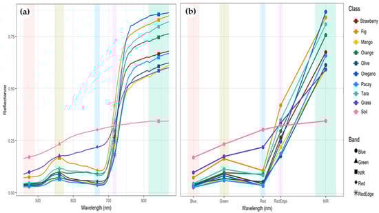
Figure 7. Average spectral signatures (endmembers) of crops and soil covers obtained with (a) FieldSpec HandHeld FSHH 325–1075P and (b) Altum PT sensor.

Figure 8 shows the Pearson correlation matrix between the 15 covariates derived from optical (Sentinel-2), radar (Sentinel-1), and topographic (DEM) data used for the classification of olive, oregano, orange, and other uses. In general, the correlations were low to moderate, indicating adequate independence between predictors. Negative correlations were observed between elevation and optical indices (ARVI, greenness, wetness), reflecting a reduction in vigor and water content at higher elevations. The optical variables (ARVI, MTCI, greenness) showed positive correlations with each other, evidencing their relationship with photosynthetic activity and chlorophyll content, while radar metrics (VH_d_corr, VH_d_asm, VH_d_contrast, ratio_VH/VV) provided complementary information on canopy structure and surface roughness, being poorly correlated with optical metrics. This combination of covariates made it possible to reduce multicollinearity (|r| > 0.75) and select an optimal set of 15 predictors, ensuring a balanced representation of the spectral, structural, and topographic factors relevant to classification in arid environments.

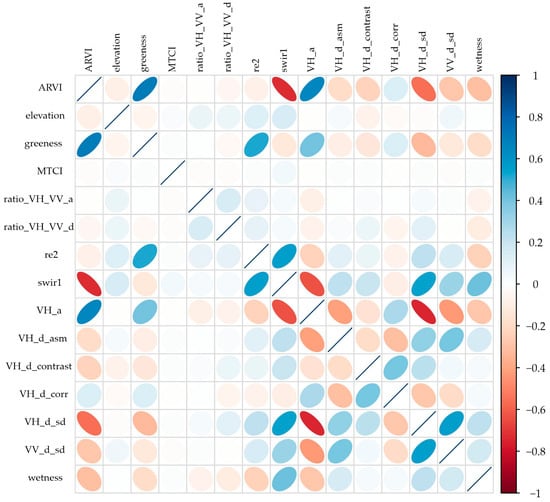
Figure 8. Decorrelation matrix between the 15 covariates selected for crop classification.

3.2. Olive Cover Mapping

The evaluation of maps obtained using CART, RF, and GTB algorithms showed consistent and high-precision performance in the classification of crops and covers present in the study area (Table 1). The CART model achieved an F1 value of 0.81, an OA of 0.83%, and a Kappa coefficient of 0.75, showing adequate discrimination of the main agricultural classes, although with slight confusion between spectrally similar covers. In contrast, the RF model presented superior performance with an F1 of 0.85, OA of 0.87, and Kappa of 0.80, demonstrating greater stability and generalization capacity. The best performance corresponded to the XGBoost model, with an F1 of 0.86, OA of 0.86, and Kappa of 0.81, confirming its effectiveness in class separation under conditions of spectral and textural heterogeneity.

Table 1. Validation metrics for olive grove coverage mapping.

Model	F1	OA	Kappa	QD	AD
CART	0.81	0.83	0.75	0.03	0.14
RF	0.85	0.87	0.80	0.03	0.11
GTB	0.86	0.86	0.81	0.03	0.11

The cartographic results of the ensemble integration (Table 2 and Figure 9) showed that areas dominated by olive trees represented the largest agricultural coverage (23,059.87 ha, 38.21%), concentrated in the central and southern zones, covering approximately the largest proportion of the total cultivated area. Orange areas (725.74 ha, 1.20%) were mainly located in intermediate zones with high reflectance in the visible range, while oregano (5352.10 ha, 8.87%) was distributed in scattered patches associated with arid soils and fine texture. Areas classified as other uses (31,207.71 ha, 51.72%) included sectors with urban areas, water bodies, and bare surfaces.

Table 2. Land use and land cover surface for the study area.

Vegetation Cover and Land Use	Area (m2)	Area (ha)	Percentage (%)
Olive	230,598,663.43	23,059.87	38.21
Oregano	53,521,040.18	5352.10	8.87
Orange	7,257,395.90	725.74	1.20
Others	312,077,058.56	31,207.71	51.72
Total	603,454,158.07	60,345.42	100.00

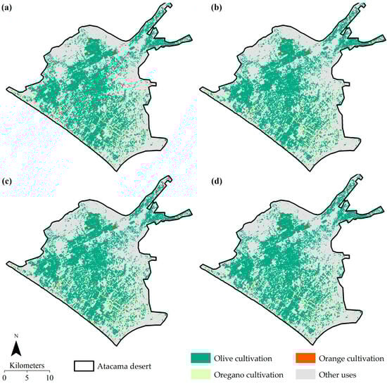
Figure 9. Land use and land cover map in the Atacama Desert based on algorithms (a) CART, (b) RF, (c) GTB, and (d) average ensemble.

3.3. Olive Trees Counting and Density

3.3.1. Decorrelation Analysis Between Model Predictors for Olive Density Mapping

Of the 48 initial environmental and spectral covariates considered to model the distribution and density of olive crops, Pearson correlation analysis (r) allowed the selection of 16 variables (Figure 10) with low collinearity and high predictive relevance: ARVI elevation, greenness, MTCI, VH_VV_ratio, VH_VV_d_ratio, re2, VH_d_asm, VH_d_contrast, VH_d_corr, VH_d_idm, VH_d_sd, VH_d_sent, VV_a, VV_d_sd, and humidity. These covariates combine spectral (optical and radar), topographic, and structural information, reflecting the biophysical and geomorphological conditions of the study area. Overall, moderate negative correlations were observed between elevation-related variables and vegetation indices, suggesting altitudinal gradients influencing crop cover and vigor. Similarly, radar texture metrics showed positive correlations with optical moisture and structure variables, indicating sensitivity to surface roughness and canopy density. The final selection of non-redundant covariates reduced model dimensionality, avoided overfitting problems, and improved the stability of the machine learning algorithms applied to olive grove classification and density estimation.

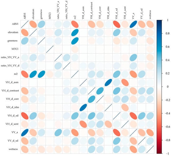
Figure 10. Correlation coefficients between class elements and model predictors. R-Pearson correlation coefficient, significant at 5% probability; X-not significant.

3.3.2. Hyperparameters

Table 3 presents the optimal hyperparameters adjusted for the CART, RF, and GTB models used to estimate olive plantation density through classification and regression. To ensure transparency and reproducibility, it should be noted that the optimization was performed using the tune_grid and tune_bayes procedures of the tidy models package in R, combining random search and Bayesian optimization with 5-fold cross-validation. The initial hyperparameter ranges were defined based on previous studies of woody crop and coffee mapping, adjusted to the spectral, radar, and topographic structure of our covariates.

Table 3. Hyperparameters for regression metrics for olive counting.

Model	Hyperparameter	Value Classification	Value Regression
RF	trees	1000	1000
	mtry	17	5
	min_n	30	2
CART	min_n	21	8
	cost_complexity	2.37 × 10−7	0
	tree_depth	8	13
GTB	min_n	14	30
	tree_depth	10	12
	trees	1641	872
	learn_rate	0.004	0.06
	loss_reduction	0.27	0.07
	sample_size	0.88	0.35

The final selection of hyperparameters was based on the average R² and RMSE performance in the validation folds, prioritizing configurations with low variability between iterations, thus ensuring stability and generalizability. In the RF model, a high number of trees (1000) was maintained in both classification and regression, which reduced the model variance and stabilized the predictions. However, the optimal mtry value differed between tasks (17 for classification and 5 for regression), indicating that continuous density prediction requires a smaller subset of random predictors per tree to improve its generalizability. In the case of CART, the greater tree depth in regression (tree_depth = 13) compared to classification (tree_depth = 8) reflects the need to capture a more complex structure in the spatial variability of olive tree density, while the near-zero cost complexity indicates minimal tree pruning. Finally, GTB showed the most adaptable behavior: in classification, it required a large number of iterations (1641 trees) and a very low learning rate (0.004) to ensure stable convergence, while in regression, it needed fewer trees (872) but with a higher learning rate (0.06), which accelerated optimization and enhanced its predictive performance.

3.3.3. Counting by Regression

The evaluation of regression models showed notable differences in predictive capacity among the three applied algorithms (CART, RF, and GTB) (Table 2). The CART model presented moderate performance, with values of MAE = 0.482, RMSE = 0.723, and R² = 0.682, reflecting lower explanatory capacity and greater error dispersion. Its RPD value = 1.76 indicates acceptable accuracy for exploratory purposes, although limited for robust quantitative predictions. In contrast, the RF model obtained R² = 0.893, accompanied by reduced errors (MAE = 0.265 and RMSE = 0.450), which demonstrates a better fit between observed and estimated values. Its RPD = 2.82 suggests excellent performance and high generalization capacity, consolidating its effectiveness for spatial estimation of olive density (Table 4).

Table 4. Validation metrics for estimating tree density using regression models.

Model	MAE	RMSE	RS2	RPD
CART	0.482	0.7238	0.682	1.76
RF	0.265	0.4508	0.893	2.82
GTB	0.258	0.443	0.885	2.87

The GTB algorithm showed very similar behavior to RF, reaching R² = 0.885, MAE = 0.258, RMSE = 0.443, and RPD = 2.87, values that confirm its high predictive power and stability. Overall, the results indicate that both RF and GTB far exceed CART, providing more accurate and consistent estimates of olive plantation density, with potential for applications in detailed mapping and productivity modeling (Table 3).

Residual analysis showed different behaviors among the models evaluated. In CART, the residuals showed greater dispersion and a structured pattern, indicating limitations in adequately capturing the continuous variability of olive tree density (Figure 11a). In contrast, RF and GTB exhibited narrower residuals centered around zero, with no systematic trends, suggesting a better ability to model nonlinear relationships and reduce variance (Figure 11b,c). Histograms and Q–Q plots show that RF and GTB generate more symmetrical distributions closer to normality, reflecting more stable and consistent predictions.

Figure 11. Residual analysis for (a) CART, (b) RF, and (c) GTB models in olive tree density estimation using residuals vs. fitted and residual distribution.

3.3.4. Counting by Classification

Table 5 summarizes the validation metrics of the classification models applied to olive density estimation. Overall, all three algorithms showed moderate performance, with F1 values between 0.30 and 0.31 and an OA below 50%, reflecting the spectral and structural complexity of the arid landscape. The CART model presented the lowest results (OA = 0.46, Kappa = 0.13), while RF achieved the highest accuracy (OA = 0.48, Kappa = 0.15) and GTB showed similar behavior (F1 = 0.31, OA = 0.47, Kappa = 0.14). The QD (0.17–0.19) and AD (0.33–0.37) metrics indicate moderate errors in quantity and spatial allocation.

Table 5. Validation metrics for estimating tree density using classification models.

Model	F1	OA	Kappa	QD	AD
CART	0.30	0.46	0.13	0.17	0.37
RF	0.30	0.48	0.15	0.19	0.33
GTB	0.31	0.47	0.14	0.17	0.35

3.3.5. Olive Crop Density Maps

The density maps generated using the CART, RF, GTB algorithms and their ensemble model (Figure 12) show a spatial correspondence consistent with field observations. In general, the areas with the highest density of plantations are concentrated in the central, northern, and northeastern sectors of the study area. This could be related to higher altitudes, deeper soils, and microclimatic conditions favorable to olive tree development. In contrast, areas with medium or low density are located towards the margins of the desert and urban areas, where soil and water limitations restrict tree cover. Among the models applied, RF and GTB presented a more homogeneous spatial distribution consistent with the actual structure of the plantations, while CART showed a greater dispersion of values at the boundaries of the agricultural area.

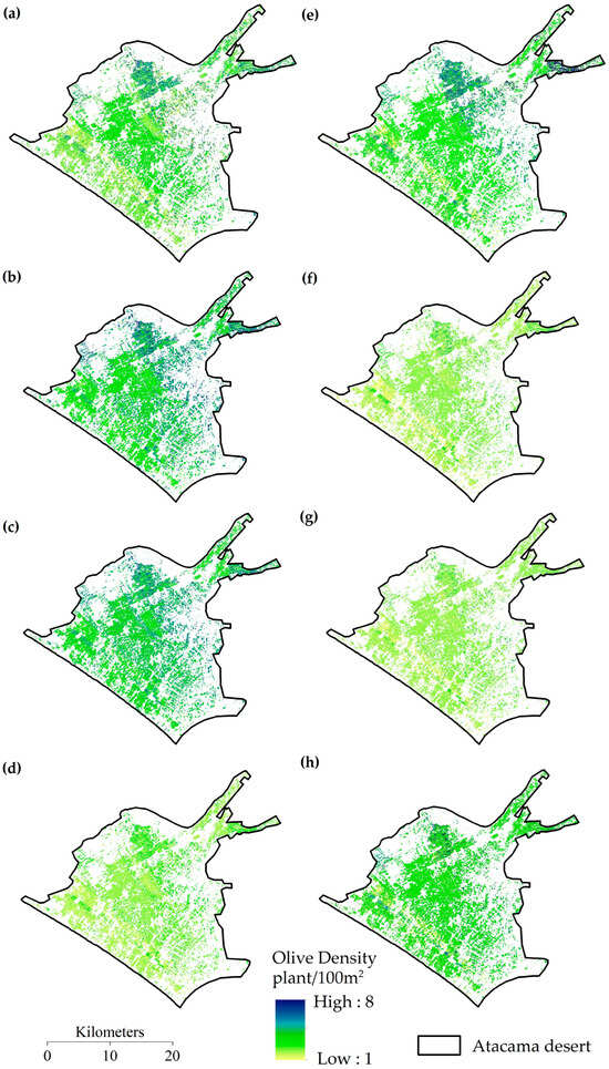
Figure 12. Olive plantation density map based on algorithms (a) CART, (b) RF, (c) GTB, and (d) mean for regression and (e) CART, (f) RF, (g) GTB, and (h) ensemble for classification.

4. Discussion

In this research, the spatial distribution of olive cultivation and its density were mapped with high precision (OA > 83%) in an arid zone of southern Peru. For this, spectral signatures, UAV multispectral data, and optical and radar satellite images were integrated. Obtaining spectral signatures of olive crop, oregano, orange, and other uses (bare soil) was key for this study, which allowed us to obtain an ideal difference to discriminate cover types in the study area. Therefore, we opted to evaluate the potential of Sentinel-1 and Sentinel-2 images to map the spatial distribution of olive cultivation.

This research work is a first attempt for large-scale mapping of olive-growing regions in the department of Tacna. The use of the GEE platform allowed using optical, textural information, and temporal metrics of radar data [58]. The combination of multiple sensors such as Sentinel-2 and Sentinel-1 can provide structural and spectral information for diverse agricultural and forest mapping tasks. Sentinel-2 with a spatial resolution of 10–20 m and a revisit time of five days allows capturing the intra-annual variability of spectral reflectance of plants, their phenological stage, and detecting tree crops [75]. Meanwhile, Sentinel-1 with spatial resolution up to 10 m in different scene polarizations and instrument modes. This provides additional structural information on the geometric orientation of plants, roughness, and water content, which can help distinguish trees from other types of vegetation [76,77,78]. In this study, the integration of Sentinel-2 and Sentinel-1 images allowed mapping vegetation cover and land use accurately and with high spectral difference with results similar to other studies [79,80,81,82].

The integration of optical, radar, and topographic data allowed generating an initial set of 48 covariates, of which, after applying a correlation threshold (|r| > 0.75) to reduce multicollinearity, 15 variables with greater explanatory relevance were selected. Optical indices derived from Sentinel-2 such as ARVI, Greenness, and MTCI provided information on vegetative vigor, photosynthetic activity, and chlorophyll content, being fundamental for discriminating areas with active vegetation against bare soils [83,84,85]. Radar metrics obtained from Sentinel-1, including VH/VV ratios and GLCM textures (contrast, correlation, entropy, homogeneity, and variance), offered structural information of the canopy, useful for characterizing roughness and foliar density under conditions of high surface reflectance or cloudiness [54,57,86]. Likewise, topographic variables derived from the digital elevation model, such as elevation, incorporated the physical component of the landscape, relevant in the distribution and productivity of olive groves in arid zones [87,88,89,90]. Overall, the combination of optical, radar, and topographic covariates strengthened the discriminative capacity of classification and regression models, technically supporting the detection and spatial characterization of olive groves in the Atacama Desert.

Machine learning algorithms such as CART, RF, and GTB have been widely used for mapping crops, vegetation cover, and land use [75]. However, individual classifiers can have limitations associated with overfitting, low capacity to represent complex patterns, and high computational demands on large datasets [91,92]. Therefore, recent studies have prioritized tree assembly-based approaches that combine multiple weak models to improve classification accuracy and robustness [48,76,93]. In our study, ensemble algorithms (RF and GTB) clearly outperformed CART, reflecting their lower variance and greater capacity to model nonlinear relationships in highly heterogeneous landscapes. The values obtained (F1 ≈ 0.85–0.86; OA ≈ 86%; Kappa ≈ 0.80–0.81) demonstrate robust discrimination between olive, orange, oregano, and other land uses, with confusion levels consistent with the spectral similarity between land covers with comparable foliage architecture.

The observed differences between the high accuracy of the land cover classification (OA ≈ 86%) and the moderate accuracy achieved in the density estimation (OA ≈ 0.47) are due to the fundamentally different nature of both tasks and the intrinsic limitations of the available data. While classification benefits from well-defined spectral patterns among crop types, density estimation requires capturing much more subtle intraspecific variations, influenced by canopy geometry, shade-to-light ratios, phenology, water status, and soil heterogeneity [94,95]. These sources of variability introduce radiometric dispersion that more significantly affects regression models. In this context, RF and GTB consistently outperformed CART due to their internal variance reduction and sequential error correction mechanisms, while CART, relying on a single tree, showed greater sensitivity to local noise and outliers. These algorithmic differences explain the drop in performance in density estimation and support the superiority of RF and GTB to represent continuous gradients associated with the spatial structure of the olive grove under arid conditions.

On the other hand, in regression, RF and GTB achieved R² = 0.89 and RPD > 2.8, indicating excellent predictive capacity for estimating tree density; in contrast, CART showed moderate fit (RPD ≈ 1.76), reflecting its greater sensitivity to input variability. In this study, the manual counting of olive and orange trees was an essential source of data for calibrating the regression model; however, visual identification can be affected by factors such as canopy overlap, variations in the illumination of the UAV mosaics, or the presence of young trees with less defined spectral signatures. To minimize these effects, internal verification procedures based on duplicate counts and comparative review between interpreters were applied, although it is acknowledged that any residual error in the counts tends to propagate to the model fitting metrics [51,96]. Similarly, temporal and geometric consistency checks were performed on the UAV images, since variability due to lighting and viewing angle can alter canopy definition and, consequently, the accuracy of manual identification.

Furthermore, it is important to contextualize our results against recent studies employing deep learning architectures based on convolutional neural networks (CNNs) for individual tree mapping in olive groves and other woody crops. While these techniques have demonstrated high efficacy for canopy detection and segmentation at the tree scale, their application relies heavily on very high-resolution imagery and extensive, meticulously annotated training sets, which increases computational costs and operational complexity [51,96]. Likewise, CNNs show their greatest strength in the detailed characterization of canopy structure, but not necessarily in generating continuous density maps at a regional scale, where multispectral and satellite radar data are more suitable. In this context, the choice of classical machine learning methods such as RF and GTB was justified both by the availability of Sentinel-1/2 and UAV data and by the need to produce robust and generalizable estimates across a broad arid landscape, while maintaining an appropriate balance between performance, interpretability, and computational efficiency. Density maps locate the highest olive concentrations in flat and low areas, consistent with favorable edaphic and water conditions; densities decrease toward slopes and margins with water/soil limitations. Various environmental and sample design factors also influence model performance and partly explain the difference between high accuracy in land cover classification and moderate accuracy in density estimation. The geometry of the sun, sensor, and illumination angle can modify the proportion of shaded and illuminated areas within the canopy, particularly affecting the red-edge and NIR bands and generating radiometric variability not associated with actual changes in tree density. Similarly, phenological changes between plots and dates related to vegetative state, fruit load, or water stress could alter the spectral response of the canopy, introducing additional noise into the relationships between vegetation indices and density. On the other hand, UAV sampling focused on accessible areas with a high presence of olive trees, so some types of plantations (e.g., very young, very scattered, or extremely stressed olive groves) may be underrepresented. These factors combined contribute to the residual dispersion observed in the regression models and to the local over- or underestimation of density, so it is recommended to incorporate multi-temporal campaigns, more rigorous lighting corrections, and spatially more balanced sampling designs in future work.

Despite the good results obtained, this study may have some limitations that should be considered when interpreting olive tree coverage and density maps. First, the analysis is based on a single time window, so the relationships found between spectral/radar covariates and plantation density could vary throughout the crop’s phenological cycle. Second, although the UAV sampling area is representative of the main production systems, it does not comprehensively cover all the management, age, and vigor gradients present in the Atacama Desert, which may limit the spatial generalization capacity of the models. Furthermore, the absence of high-resolution edaphic covariates, particularly direct indicators of soil salinity and moisture content, limits the ability to explicitly capture some key processes in arid environments. In this regard, future research should integrate complete multi-temporal Sentinel-1/2 series, detailed soil information (e.g., maps of electrical conductivity and soil moisture), and additional UAV campaigns (with multispectral sensors and LiDAR) in underrepresented strata, as well as explore hybrid approaches that combine assembly models with deep learning architectures (CNN + ensemble models) to improve both the counting and structural characterization of plantations.

5. Conclusions

The combination of UAVs and satellites with machine learning enabled high-precision mapping of agricultural coverage and reliable estimation of olive tree density in the Atacama Desert (Tacna, Peru). Assembly models, particularly RF and GTB, offered the best performance in classification (OA ≈ 86%; Kappa ≈ 0.80) and regression (R² ≈ 0.89; RPD > 2.8), significantly outperforming CART. The final selection of 15 covariates combining optical, radar, and topographic data reduced dimensionality and improved model stability and generalization.

The density maps obtained reflected spatial patterns consistent with the actual distribution of the crop: higher concentrations in the low, flat areas of the desert and a progressive decrease towards areas with steeper slopes and water limitations. Overall, the results confirm the methodological soundness of the proposed approach for characterizing agricultural systems in arid environments. Furthermore, although its effectiveness was tested under the particular conditions of the Atacama Desert, the modular structure of the covariates used and the use of tree-based models suggest a high potential for transferability to other woody crops and regions with similar environmental conditions.

References

- Blanco, I.; De Bellis, L.; Luvisi, A. Bibliometric Mapping of Research on Life Cycle Assessment of Olive Oil Supply Chain. Sustainability 2022, 14, 3747. [Google Scholar] [CrossRef]
- El Bakkali, A.; Haouane, H.; Moukhli, A.; Costes, E.; van Damme, P.; Khadari, B. Construction of Core Collections Suitable for Association Mapping to Optimize Use of Mediterranean Olive (Olea europaea L.) Genetic Resources. PLoS ONE 2013, 8, e61265. [Google Scholar] [CrossRef] [PubMed]
- Navarro, R.; Wirkus, L.; Dubovyk, O. Spatio-Temporal Assessment of Olive Orchard Intensification in the Saïss Plain (Morocco) Using k-Means and High-Resolution Satellite Data. Remote Sens. 2023, 15, 50. [Google Scholar] [CrossRef]
- Commissiones Europea. Olio Di Oliva. Available online: https://agriculture.ec.europa.eu/farming/crop-productions-and-plant-based-products/olive-oil_it (accessed on 15 May 2025).
- Stempfle, S.; Carlucci, D.; de Gennaro, B.C.; Roselli, L.; Giannoccaro, G. Available Pathways for Operationalizing Circular Economy into the Olive Oil Supply Chain: Mapping Evidence from a Scoping Literature Review. Sustainability 2021, 13, 9789. [Google Scholar] [CrossRef]
- Choudri, B.; Charabi, Y.; Ahmed, M. Pesticides and Herbicides. Water Environ. Res. 2018, 90, 1663–1678. [Google Scholar] [CrossRef]
- Mahmood, I.; Imadi, S.R.; Shazadi, K.; Gul, A.; Hakeem, K.R. Effects of Pesticides on Environment. In Plant, Soil Microbes; Springer: Cham, Switzerland, 2016; pp. 253–269. [Google Scholar] [CrossRef]
- Karydas, C.G.; Sekuloska, T.; Silleos, G.N. Quantification and Site-Specification of the Support Practice Factor when Mapping Soil Erosion Risk Associated with Olive Plantations in the Mediterranean Island of Crete. Environ. Monit. Assess. 2009, 149, 19–28. [Google Scholar] [CrossRef]
- Brito, C.; Dinis, L.-T.; Moutinho-Pereira, J.; Correia, C.M. Drought Stress Effects and Olive Tree Acclimation under a Changing Climate. Plants 2019, 8, 232. [Google Scholar] [CrossRef]
- Vargas, E.M.P.; Ascencios, D.R. Sustainability of Olive Cultivation under a Climatological Approach in an Arid Region at the Atacama Desert. Cienc. Tecnol. Agropecu. 2022, 23, e2652. [Google Scholar] [CrossRef]
- Machaca, R.P.; Pino, E.V.; Ramos, L.F.R.; Quile, J.M.; Torres, A.R. Estimación de La Evapotranspiración Con Fines de Riego En Tiempo Real de Un Olivar a Partir de Imágenes de Un Drone En Zonas Áridas, Caso La Yarada, Tacna, Perú. Idesia 2022, 40, 55–65. [Google Scholar] [CrossRef]
- Izaguirre-Malasquez, R.; Muñoz-Gonzales, L.; Cabel-Pozo, J.; Raymundo, C. Inventory Optimization Model Applying the FIFO Method and the PHVA Methodology to Improve the Stock Levels of Olive Products in SMEs of the Agro-Industrial Sector in Peru; Springer Science and Business Media Deutschland GmbH: Berlin, Germany, 2022; ISBN 9783030855390. [Google Scholar]
- Casanova, D.P. Guía Técnica Del Cultivo de En La Región Tacna; Instituto Nacional de Innovación Agraria: Lima, Perú, 2019. [Google Scholar]
- Abahous, H.; Bouchaou, L.; Chehbouni, A. Global Climate Pattern Impacts on Long-Term Olive Yields in Northwestern Africa: Case from Souss-Massa Region. Sustainability 2021, 13, 1340. [Google Scholar] [CrossRef]
- Xiong, J.; Thenkabail, P.S.; Gumma, M.K.; Teluguntla, P.; Poehnelt, J.; Congalton, R.G.; Yadav, K.; Thau, D. Automated Cropland Mapping of Continental Africa Using Google Earth Engine Cloud Computing. ISPRS J. Photogramm. Remote Sens. 2017, 126, 225–244. [Google Scholar] [CrossRef]
- Yun, T.; Jiang, K.; Li, G.; Eichhorn, M.P.; Fan, J.; Liu, F.; Chen, B.; An, F.; Cao, L. Individual Tree Crown Segmentation from Airborne LiDAR Data Using a Novel Gaussian Filter and Energy Function Minimization-Based Approach. Remote Sens. Environ. 2021, 256, 112307. [Google Scholar] [CrossRef]
- Ferreira, M.P.; de Almeida, D.R.A.; Papa, D.D.A.; Minervino, J.B.S.; Veras, H.F.P.; Formighieri, A.; Santos, C.A.N.; Ferreira, M.A.D.; Figueiredo, E.O.; Ferreira, E.J.L. Individual Tree Detection and Species Classification of Amazonian Palms Using UAV Images and Deep Learning. For. Ecol. Manag. 2020, 475, 118397. [Google Scholar] [CrossRef]
- Vatandaslar, C.; Lee, T.; Bettinger, P.; Ucar, Z.; Stober, J.; Peduzzi, A. Mapping Percent Canopy Cover Using Individual Tree- and Area-Based Procedures that Are Based on Airborne LiDAR Data: Case Study from an Oak-Hickory-Pine Forest in the USA. Ecol. Indic. 2024, 167, 112710. [Google Scholar] [CrossRef]
- Lin, C.; Zhou, J.; Yin, L.; Bouabid, R.; Mulla, D.; Benami, E.; Jin, Z. Sub-National Scale Mapping of Individual Olive Trees Integrating Earth Observation and Deep Learning. ISPRS J. Photogramm. Remote Sens. 2024, 217, 18–31. [Google Scholar] [CrossRef]
- Jurado, J.M.; Ortega, L.; Cubillas, J.J.; Feito, F.R. Multispectral Mapping on 3D Models and Multi-Temporal Monitoring for Individual Characterization of Olive Trees. Remote Sens. 2020, 12, 1106. [Google Scholar] [CrossRef]
- Kelley, L.C.; Pitcher, L.; Bacon, C. Using Google Earth Engine to Map Complex Shade-Grown Coffee Landscapes in Northern Nicaragua. Remote Sens. 2018, 10, 952. [Google Scholar] [CrossRef]
- Xu, Y.; Yu, L.; Li, W.; Ciais, P.; Cheng, Y.; Gong, P. Annual Oil Palm Plantation Maps in Malaysia and Indonesia from 2001 to 2016. Earth Syst. Sci. Data 2020, 12, 847–867. [Google Scholar] [CrossRef]
- Mubin, N.A.; Nadarajoo, E.; Shafri, H.Z.M.; Hamedianfar, A. Young and Mature Oil Palm Tree Detection and Counting Using Convolutional Neural Network Deep Learning Method. Int. J. Remote Sens. 2019, 40, 7500–7515. [Google Scholar] [CrossRef]
- Li, Z.; Fox, J.M. Integrating Mahalanobis Typicalities with a Neural Network for Rubber Distribution Mapping. Remote Sens. Lett. 2011, 2, 157–166. [Google Scholar] [CrossRef]
- Maes, W.H.; Steppe, K. Perspectives for Remote Sensing with Unmanned Aerial Vehicles in Precision Agriculture. Trends Plant Sci. 2019, 24, 152–164. [Google Scholar] [CrossRef]
- Li, W.; Dong, R.; Fu, H.; Yu, L. Large-Scale Oil Palm Tree Detection from High-Resolution Satellite Images Using Two-Stage Convolutional Neural Networks. Remote Sens. 2019, 11, 11. [Google Scholar] [CrossRef]
- Ameslek, O.; Zahir, H.; Latifi, H.; Bachaoui, E.M. Combining OBIA, CNN, and UAV Imagery for Automated Detection and Mapping of Individual Olive Trees. Smart Agric. Technol. 2024, 9, 100546. [Google Scholar] [CrossRef]
- Lin, C.; Jin, Z.; Mulla, D.; Ghosh, R.; Guan, K.; Kumar, V.; Cai, Y. Toward Large-Scale Mapping of Tree Crops with High-Resolution Satellite Imagery and Deep Learning Algorithms: A Case Study of Olive Orchards in Morocco. Remote Sens. 2021, 13, 1740. [Google Scholar] [CrossRef]
- Ferrer-Vilca, T.H.; Valverde-Rodríguez, A. Rendimiento Del Frejol (Phaseolus vulgaris L.) Variedad Canario Con Tres Fuentes de Abonos Orgánicos En El Distrito de Cholón, Huánuco-Perú. Rev. Investig. Agrar. 2020, 2, 33–44. [Google Scholar] [CrossRef]
- Barboza, E.; Salazar, W.; Gálvez-Paucar, D.; Valqui-Valqui, L.; Saravia, D.; Gonzales, J.; Aldana, W.; Vásquez, H.V.; Arbizu, C.I. Cover and Land Use Changes in the Dry Forest of Tumbes (Peru) Using Sentinel-2 and Google Earth Engine Data. Environ. Sci. Proc. 2022, 22, 2. [Google Scholar] [CrossRef]
- Villalobos, F.; Testi, L.; Hidalgo, J.; Pastor, M.; Orgaz, F. Modelling Potential Growth and Yield of Olive (Olea europaea L.) Canopies. Eur. J. Agron. 2006, 24, 296–303. [Google Scholar] [CrossRef]
- Kebede, B.; Soromessa, T. Allometric Equations for Aboveground Biomass Estimation of Olea europaea L. subsp. Cuspidata in Mana Angetu Forest. Ecosyst. Health Sustain. 2018, 4, 1–12. [Google Scholar] [CrossRef]
- Contreras, F.; Cayuela, M.L.; Sánchez-Monedero, M.A.; Pérez-Cutillas, P. Multi-Source Remote Sensing for Large-Scale Biomass Estimation in Mediterranean Olive Orchards Using GEDI LiDAR and Machine Learning. Biogeosciences 2025, 22, 7625–7646. [Google Scholar] [CrossRef]
- Fernández-Sarría, A.; López-Cortés, I.; Estornell, J.; Velázquez-Martí, B.; Salazar, D. Estimating Residual Biomass of Olive Tree Crops Using Terrestrial Laser Scanning. Int. J. Appl. Earth Obs. Geoinf. 2019, 75, 163–170. [Google Scholar] [CrossRef]
- Pino, V.E.; Montalván, D.I.; Vera, M.A.; Ramos, F.L. La Conductancia Estomática y Su Relación Con La Temperatura Foliar y Humedad Del Suelo En El Cultivo Del Olivo (Olea europaea L.), En Periodo de Maduración de Frutos, En Zonas Áridas. La Yarada, Tacna, Perú. Idesia 2019, 37, 55–64. [Google Scholar] [CrossRef]
- Gallardo-Salazar, J.L.; Pompa-García, M. Detecting Individual Tree Attributes and Multispectral Indices Using Unmanned Aerial Vehicles: Applications in a Pine Clonal Orchard. Remote Sens. 2020, 12, 4144. [Google Scholar] [CrossRef]
- Alganci, U.; Sertel, E.; Kaya, S. Determination of the Olive Trees with Object Based Classification of Pleiades Satellite Image. Int. J. Environ. Geoinformatics 2018, 5, 132–139. [Google Scholar] [CrossRef]
- Weissteiner, C.J.; Strobl, P.; Sommer, S. Assessment of Status and Trends of Olive Farming Intensity in EU-Mediterranean Countries Using Remote Sensing Time Series and Land Cover Data. Ecol. Indic. 2011, 11, 601–610. [Google Scholar] [CrossRef]
- Khan, A.; Khan, U.; Waleed, M.; Khan, A.; Kamal, T.; Marwat, S.N.K.; Maqsood, M.; Aadil, F. Remote Sensing: An Automated Methodology for Olive Tree Detection and Counting in Satellite Images. IEEE Access 2018, 6, 77816–77828. [Google Scholar] [CrossRef]
- Roma, E.; Catania, P.; Vallone, M.; Orlando, S. Unmanned Aerial Vehicle and Proximal Sensing of Vegetation Indices in Olive Tree (Olea europaea). J. Agric. Eng. 2023, 54, 1536. [Google Scholar] [CrossRef]
- Šiljeg, A.; Marinović, R.; Domazetović, F.; Jurišić, M.; Marić, I.; Panđa, L.; Radočaj, D.; Milošević, R. GEOBIA and Vegetation Indices in Extracting Olive Tree Canopies Based on Very High-Resolution UAV Multispectral Imagery. Appl. Sci. 2023, 13, 739. [Google Scholar] [CrossRef]
- Šiljeg, A.; Panđa, L.; Domazetović, F.; Marić, I.; Gašparović, M.; Borisov, M.; Milošević, R. Comparative Assessment of Pixel and Object-Based Approaches for Mapping of Olive Tree Crowns Based on UAV Multispectral Imagery. Remote Sens. 2022, 14, 757. [Google Scholar] [CrossRef]
- Vargas, E.M.P.; Huayna, G. Spatial and Temporal Evolution of Olive Cultivation Due to Pest Attack, Using Remote Sensing and Satellite Image Processing. Sci. Agropecu. 2022, 13, 149–157. [Google Scholar] [CrossRef]
- SENAMHI. Climas del Perú: Mapa de Clasificación Climática Nacional. Lima, Perú. 2010. Available online: https://www.senamhi.gob.pe/load/file/01404SENA-4.pdf (accessed on 10 October 2025).
- MINAM. Procedimiento Técnico y Metodológico para la Elaboración del “Estudio Especializado de Análisis de los Cambios de la Cobertura y Uso de la Tierra”; MINAM: Lima, Perú, 2016. [Google Scholar]
- Pino, V.E. Conflictos por el uso del agua en una región árida: Caso Tacna, Perú. Diálogo Andin. 2021, 65, 405–415. [Google Scholar] [CrossRef]
- MapBiomas Maps de Cobertura y Uso. Available online: https://peru.mapbiomas.org/colecciones-de-mapbiomas-peru/ (accessed on 10 October 2025).
- Pizarro, S.; Pricope, N.G.; Figueroa, D.; Carbajal, C.; Quispe, M.; Vera, J.; Alejandro, L.; Achallma, L.; Gonzalez, I.; Salazar, W.; et al. Implementing Cloud Computing for the Digital Mapping of Agricultural Soil Properties from High Resolution UAV Multispectral Imagery. Remote Sens. 2023, 15, 3203. [Google Scholar] [CrossRef]
- Hao, Z.; Lin, L.; Post, C.J.; Mikhailova, E.A.; Li, M.; Chen, Y.; Yu, K.; Liu, J. Automated Tree-Crown and Height Detection in a Young Forest Plantation Using Mask Region-Based Convolutional Neural Network (Mask R-CNN). ISPRS J. Photogramm. Remote Sens. 2021, 178, 112–123. [Google Scholar] [CrossRef]
- Schiefer, F.; Kattenborn, T.; Frick, A.; Frey, J.; Schall, P.; Koch, B.; Schmidtlein, S. Mapping Forest Tree Species in High Resolution UAV-Based RGB-Imagery by Means of Convolutional Neural Networks. ISPRS J. Photogramm. Remote Sens. 2020, 170, 205–215. [Google Scholar] [CrossRef]
- Yu, K.; Hao, Z.; Post, C.J.; Mikhailova, E.A.; Lin, L.; Zhao, G.; Tian, S.; Liu, J. Comparison of Classical Methods and Mask R-CNN for Automatic Tree Detection and Mapping Using UAV Imagery. Remote Sens. 2022, 14, 295. [Google Scholar] [CrossRef]
- Gorelick, N.; Hancher, M.; Dixon, M.; Ilyushchenko, S.; Thau, D.; Moore, R. Google Earth Engine: Planetary-Scale Geospatial Analysis for Everyone. Remote Sens. Environ. 2017, 202, 18–27. [Google Scholar] [CrossRef]
- Farr, T.G.; Rosen, P.A.; Caro, E.; Crippen, R.; Duren, R.; Hensley, S.; Kobrick, M.; Paller, M.; Rodriguez, E.; Roth, L.; et al. The Shuttle Radar Topography Mission. Rev. Geophys. 2007, 45, RG2004. [Google Scholar] [CrossRef]
- Lelong, C.C.D.; Thong-Chane, A. Application of Textural Analysis on Very High Resolution Panchromatic Images to Map Coffee Orchards in Uganda. In Proceedings of the IGARSS 2003. 2003 IEEE International Geoscience and Remote Sensing Symposium. Proceedings (IEEE Cat. No. 03CH37477), Toulouse, France, 21–25 July 2003; Volume 3, pp. 1007–1009. [Google Scholar] [CrossRef]
- Drielsma, M.J.; Love, J.; Taylor, S.; Thapa, R.; Williams, K.J. General Landscape Connectivity Model (GLCM): A New Way to Map Whole of Landscape Biodiversity Functional Connectivity for Operational Planning and Reporting. Ecol. Model. 2022, 465, 109858. [Google Scholar] [CrossRef]
- Moreira, E.P.; Valeriano, M.M. Application and Evaluation of Topographic Correction Methods to Improve Land Cover Mapping Using Object-Based Classification. Int. J. Appl. Earth Obs. Geoinf. 2014, 32, 208–217. [Google Scholar] [CrossRef]
- Haralick, R.M.; Shanmugam, K.; Dinstein, I.H. Textural Features for Image Classification. IEEE Trans. Syst. Man Cybern. 1973, SMC-3, 610–621. [Google Scholar] [CrossRef]
- Maskell, G.; Chemura, A.; Nguyen, H.; Gornott, C.; Mondal, P. Integration of Sentinel Optical and Radar Data for Mapping Smallholder Coffee Production Systems in Vietnam. Remote Sens. Environ. 2021, 266, 112709. [Google Scholar] [CrossRef]
- Delgado, E.; Barboza, E.; Rojas-Briceño, N.B.; Cotrina-Sanchez, A.; Valdés-Velásquez, A.; de la Lama, R.L.; Llerena-Cayo, C.; de la Puente, S. Modeling and Predicting Land Use and Land Cover Changes Using Remote Sensing in Tropical Coastal Ecosystems of Southern Peru. Environ. Sci. Eur. 2025, 37, 139. [Google Scholar] [CrossRef]
- Schulz, D.; Yin, H.; Tischbein, B.; Verleysdonk, S.; Adamou, R.; Kumar, N. Land Use Mapping Using Sentinel-1 and Sentinel-2 Time Series in a Heterogeneous Landscape in Niger, Sahel. ISPRS J. Photogramm. Remote Sens. 2021, 178, 97–111. [Google Scholar] [CrossRef]
- Shi, T.; Xu, H. Derivation of Tasseled Cap Transformation Coefficients for Sentinel-2 MSI At-Sensor Reflectance Data. IEEE J. Sel. Top. Appl. Earth Obs. Remote Sens. 2019, 12, 4038–4048. [Google Scholar] [CrossRef]
- Waldner, F.; Chen, Y.; Lawes, R.; Hochman, Z. Needle in a Haystack: Mapping Rare and Infrequent Crops Using Satellite Imagery and Data Balancing Methods. Remote Sens. Environ. 2019, 233, 111375. [Google Scholar] [CrossRef]
- Hasanuzzaman, M.; Adhikary, P.P.; Shit, P.K. Gully Erosion Susceptibility Mapping and Prioritization of Gully-Dominant Sub-Watersheds Using Machine Learning Algorithms: Evidence from the Silabati River (Tropical River, India). Adv. Space Res. 2023, 73, 1653–1666. [Google Scholar] [CrossRef]
- Paul, S.; Kumar, D.N. Evaluation of Feature Selection and Feature Extraction Techniques on Multi-Temporal Landsat-8 Images for Crop Classification. Remote Sens. Earth Syst. Sci. 2019, 2, 197–207. [Google Scholar] [CrossRef]
- Cao, X.; Wei, C.; Han, J.; Jiao, L. Hyperspectral Band Selection Using Improved Classification Map. IEEE Geosci. Remote Sens. Lett. 2017, 14, 2147–2151. [Google Scholar] [CrossRef]
- Jin, Z.; Azzari, G.; You, C.; Di Tommaso, S.; Aston, S.; Burke, M.; Lobell, D.B. Smallholder Maize Area and Yield Mapping at National Scales with Google Earth Engine. Remote Sens. Environ. 2019, 228, 115–128. [Google Scholar] [CrossRef]
- Auret, L.; Aldrich, C. Empirical Comparison of Tree Ensemble Variable Importance Measures. Chemom. Intell. Lab. Syst. 2011, 105, 157–170. [Google Scholar] [CrossRef]
- Breiman, L.; Friedman, J.H.; Olshen, R.A.; Stone, C.J. Classification and Regression Trees; Routledge: Boca Raton, FL, USA, 2017; pp. 1–358. [Google Scholar] [CrossRef]
- Jain, P.; Coogan, S.C.P.; Subramanian, S.G.; Crowley, M.; Taylor, S.W.; Flannigan, M.D. A Review of Machine Learning Applications in Wildfire Science and Management. Environ. Rev. 2020, 28, 478–505. [Google Scholar] [CrossRef]
- Breiman, L. Random Forests. Mach. Learn. 2001, 45, 5–32. [Google Scholar] [CrossRef]
- Hu, B.; Xue, J.; Zhou, Y.; Shao, S.; Fu, Z.; Li, Y.; Chen, S.; Qi, L.; Shi, Z. Modelling Bioaccumulation of Heavy Metals in Soil-Crop Ecosystems and Identifying Its Controlling Factors Using Machine Learning. Environ. Pollut. 2020, 262, 114308. [Google Scholar] [CrossRef] [PubMed]
- Hu, B.; Geng, Y.; Shi, K.; Xie, M.; Ni, H.; Zhu, Q.; Qiu, Y.; Zhang, Y.; Bourennane, H. Fine-Resolution Baseline Maps of Soil Nutrients in Farmland of Jiangxi Province Using Digital Soil Mapping and Interpretable Machine Learning. CATENA 2024, 249, 108635. [Google Scholar] [CrossRef]
- Chen, T.; Guestrin, C. XGBoost: A Scalable Tree Boosting System. In Proceedings of the 22nd ACM SIGKDD International Conference on Knowledge Discovery and Data Mining, San Francisco, CA, USA, 13–17 August 2016; pp. 785–794. [Google Scholar] [CrossRef]
- Pontius, R.G., Jr.; Millones, M. Death to Kappa: Birth of Quantity Disagreement and Allocation Disagreement for Accuracy Assessment. Int. J. Remote Sens. 2011, 32, 4407–4429. [Google Scholar] [CrossRef]
- Phiri, D.; Simwanda, M.; Salekin, S.; Ryirenda, V.R.; Murayama, Y.; Ranagalage, M.; Oktaviani, N.; Kusuma, H.A.; Zhang, T.; Su, J.; et al. Sentinel-2 Data For Land Cover/Use Mapping: A Review. Remote Sens. 2020, 12, 2291. [Google Scholar] [CrossRef]
- Nabil, M.; Farg, E.; Arafat, S.M.; Aboelghar, M.; Afify, N.M.; Elsharkawy, M.M. Tree-Fruits Crop Type Mapping from Sentinel-1 and Sentinel-2 Data Integration in Egypt’s New Delta Project. Remote Sens. Appl. Soc. Environ. 2022, 27, 100776. [Google Scholar] [CrossRef]
- Qiu, B.; Lin, D.; Chen, C.; Yang, P.; Tang, Z.; Jin, Z.; Ye, Z.; Zhu, X.; Duan, M.; Huang, H.; et al. From Cropland to Cropped Field: A Robust Algorithm for National-Scale Mapping by Fusing Time Series of Sentinel-1 and Sentinel-2. Int. J. Appl. Earth Obs. Geoinf. 2022, 113, 103006. [Google Scholar] [CrossRef]
- Liu, C.-A.; Chen, Z.-X.; Shao, Y.; Chen, J.-S.; Hasi, T.; Pan, H.-Z. Research Advances of SAR Remote Sensing for Agriculture Applications: A Review. J. Integr. Agric. 2019, 18, 506–525. [Google Scholar] [CrossRef]
- Felegari, S.; Sharifi, A.; Moravej, K.; Amin, M.; Golchin, A.; Muzirafuti, A.; Tariq, A.; Zhao, N. Integration of Sentinel 1 and Sentinel 2 Satellite Images for Crop Mapping. Appl. Sci. 2021, 11, 10104. [Google Scholar] [CrossRef]
- Van Tricht, K.; Gobin, A.; Gilliams, S.; Piccard, I. Synergistic Use of Radar Sentinel-1 and Optical Sentinel-2 Imagery for Crop Mapping: A Case Study for Belgium. Remote Sens. 2018, 10, 1642. [Google Scholar] [CrossRef]
- Orynbaikyzy, A.; Gessner, U.; Mack, B.; Conrad, C. Crop Type Classification Using Fusion of Sentinel-1 and Sentinel-2 Data: Assessing the Impact of Feature Selection, Optical Data Availability, and Parcel Sizes on the Accuracies. Remote Sens. 2020, 12, 2779. [Google Scholar] [CrossRef]
- Akcay, H.; Aksoy, S.; Kaya, S.; Sertel, E.; Dash, J. Evaluating the Potential of Multi-Temporal Sentinel-1 and Sentinel-2 Data for Regional Mapping of Olive Trees. Int. J. Remote Sens. 2023, 44, 7338–7364. [Google Scholar] [CrossRef]
- Bernardes, T.; Moreira, M.A.; Adami, M.; Giarolla, A.; Rudorff, B.F.T. Monitoring Biennial Bearing Effect on Coffee Yield Using MODIS Remote Sensing Imagery. Remote Sens. 2012, 4, 2492–2509. [Google Scholar] [CrossRef]
- da Silva, P.C.; Junior, W.Q.R.; Ramos, M.L.G.; Lopes, M.F.; Santana, C.C.; Casari, R.A.d.C.N.; Brasileiro, L.d.O.; Veiga, A.D.; Rocha, O.C.; Malaquias, J.V.; et al. Multispectral Images for Drought Stress Evaluation of Arabica Coffee Genotypes Under Different Irrigation Regimes. Sensors 2024, 24, 7271. [Google Scholar] [CrossRef]
- Nogueira, S.M.C.; Moreira, M.A.; Volpato, M.M.L. Relationship between Coffee Crop Productivity and Vegetation Indexes Derived from Oli/Landsat-8 Sensor Data with and without Topographic Correction. Int. Braz. Assoc. Agric. Eng. 2018, 38, 387–394. [Google Scholar] [CrossRef]
- Silva, W.F.; Rudorff, B.F.; Formaggio, A.R.; Paradella, W.R.; Mura, J.C. Discrimination of Agricultural Crops in a Tropical Semi-Arid Region of Brazil Based on L-Band Polarimetric Airborne SAR Data. ISPRS J. Photogramm. Remote Sens. 2009, 64, 458–463. [Google Scholar] [CrossRef]
- Tassew, A.A.; Yadessa, G.B.; Bote, A.D.; Obso, T.K. Influence of Location, Elevation Gradients, Processing Methods, and Soil Quality on the Physical and Cup Quality of Coffee in the Kafa Biosphere Reserve of SW Ethiopia. Heliyon 2021, 7, e07790. [Google Scholar] [CrossRef]
- Fekadu, A.; Andarege, B. Gis and Parametric Based Coffee Site Suitability Zonation in North Shewa Zone of Oromia Region, Central Ethiopia. Environ. Sustain. Indic. 2025, 26, 100674. [Google Scholar] [CrossRef]
- Liu, X.; Tan, Y.; Dong, J.; Wu, J.; Wang, X.; Sun, Z. Assessing Habitat Selection Parameters of Arabica Coffee Using BWM and BCM Methods Based on GIS. Sci. Rep. 2025, 15, 8. [Google Scholar] [CrossRef]
- López, R.S.; Fernández, D.G.; López, J.O.S.; Briceño, N.B.R.; Oliva, M.; Murga, R.E.T.; Trigoso, D.I.; Castillo, E.B.; Gurbillón, M.Á.B. Land Suitability for Coffee (Coffea Arabica) Growing in Amazonas, Peru: Integrated Use of AHP, GIS and RS. ISPRS Int. J. Geo-Inf. 2020, 9, 673. [Google Scholar] [CrossRef]
- Zhang, F.; Yang, X. Improving Land Cover Classification in an Urbanized Coastal Area by Random Forests: The Role of Variable Selection. Remote Sens. Environ. 2020, 251, 112105. [Google Scholar] [CrossRef]
- Belgiu, M.; Drăguţ, L. Random Forest in Remote Sensing: A Review of Applications and Future Directions. ISPRS J. Photogramm. Remote Sens. 2016, 114, 24–31. [Google Scholar] [CrossRef]
- Azedou, A.; Amine, A.; Kisekka, I.; Lahssini, S. Genetic Algorithm Optimization of Ensemble Learning Approach for Improved Land Cover and Land Use Mapping: Application to Talassemtane National Park. Ecol. Indic. 2025, 177, 113776. [Google Scholar] [CrossRef]
- Berger, K.; Machwitz, M.; Kycko, M.; Kefauver, S.C.; Van Wittenberghe, S.; Gerhards, M.; Verrelst, J.; Atzberger, C.; van der Tol, C.; Damm, A.; et al. Multi-Sensor Spectral Synergies for Crop Stress Detection and Monitoring in the Optical Domain: A Review. Remote Sens. Environ. 2022, 280, 113198. [Google Scholar] [CrossRef]
- Dai, J.; König, M.; Jamalinia, E.; Hondula, K.L.; Vaughn, N.R.; Heckler, J.; Asner, G.P. Canopy-Level Spectral Variation and Classification of Diverse Crop Species with Fine Spatial Resolution Imaging Spectroscopy. Remote Sens. 2024, 16, 1447. [Google Scholar] [CrossRef]
- Hnida, Y.; Mahraz, M.A.; Yahyaouy, A.; Achebour, A.; Riffi, J.; Tairi, H. Enhanced Multi-Scale Detection of Olive Tree Crowns in UAV Orthophotos Using a Deep Learning Architecture. Smart Agric. Technol. 2025, 12, 101126. [Google Scholar] [CrossRef]
Disclaimer/Publisher’s Note: The statements, opinions and data contained in all publications are solely those of the individual author(s) and contributor(s) and not of MDPI and/or the editor(s). MDPI and/or the editor(s) disclaim responsibility for any injury to people or property resulting from any ideas, methods, instructions or products referred to in the content. |
© 2026 by the authors. Licensee MDPI, Basel, Switzerland. This article is an open access article distributed under the terms and conditions of the Creative Commons Attribution (CC BY) license.