Machine Learning-Based Prediction of External Pressure in High-Speed Rail Tunnels: Model Optimization and Comparison

Abstract

The pressure fluctuations generated during high-speed train passage through tunnels can compromise both the train’s structural integrity and passenger comfort, highlighting the need for the accurate prediction of external pressure wave amplitudes. To address the high computational cost of multi-condition Computational Fluid Dynamics simulations, this study proposes a hybrid method combining numerical simulation and machine learning. A dataset was generated using simulations with five input features: tunnel length, train length, train speed, blockage ratio, and measurement point location. Four machine learning models—random forest, support vector regression, Extreme Gradient Boosting, and Multilayer Perceptron (MLP)—were evaluated, with the MLP model showing the highest baseline accuracy. To further improve performance, six metaheuristic algorithms were applied to optimize the MLP model, among which, the sparrow search algorithm (SSA) achieved the highest accuracy, with R² = 0.993, MAPE = 0.052, and RMSE = 0.112. A SHapley Additive exPlanations (SHAP) analysis indicated that the train speed and the blockage ratio were the most influential features. This study provides an effective and interpretable method for pressure wave prediction in tunnel environments and demonstrates the first integration of SSA optimization into aerodynamic pressure modeling.

1. Introduction

In recent years, high-speed trains in China have gained widespread popularity among passengers due to their advantages in speed, comfort, stability, safety, and environmental sustainability. However, with the continuous increase in operating velocities, aerodynamic challenges have become increasingly prominent [1,2]. When a high-speed train passes through a tunnel, the confined tunnel walls significantly alter the surrounding flow field, giving rise to compression and expansion waves. These pressure waves propagate at the speed of sound within the tunnel, undergoing repeated reflections and superpositions, which in turn cause cyclic fluctuations in the aerodynamic pressure on the train’s surface. Prolonged and alternating exposure to such positive and negative aerodynamic loads [3] can lead to local stress concentrations, particularly at critical structural interfaces, such as welded joints. These stress concentrations may induce fatigue damage in the welded regions and other local structures, ultimately compromising both the structural integrity of the train and passenger safety. Therefore, it is essential to investigate the characteristics of external pressure variations during high-speed train passage through tunnels, as such studies are of great significance in ensuring the safe operation of high-speed rail systems.

Extensive research has been conducted by scholars, both in China and abroad, to investigate the characteristics of the external pressure fluctuations induced by high-speed trains passing through tunnels. These studies, based on experimental investigations and numerical simulations, have provided in-depth insights into the influencing factors. The experimental results have demonstrated that the peak-to-peak value of the external pressure increases with the train formation length [4]. Moreover, both the amplitude of the external pressure variation and its peak-to-peak value have been shown to be proportional to the square of the train speed [5,6,7]. Additionally, the absolute values of the pressure peak-to-peak amplitude, maximum positive pressure, and maximum negative pressure tend to first increase and then decrease with increasing tunnel length [8]. A systematic analysis of available full-scale experimental data indicates that when the tunnel length is below a certain critical threshold, the peak-to-peak value of pressure increases with tunnel length. However, once this critical length is exceeded, the pressure fluctuation tends to reach a steady state [9].

Numerical simulation studies on the pressure waves generated by high-speed trains passing through tunnels have revealed several key patterns. It has been shown that the peak-to-peak value of external pressure is proportional to the square of train speed and exhibits an approximately linear relationship with the blockage ratio [10]. Both the amplitude and the peak-to-peak value of external pressure increase with the train formation length [11,12]. Furthermore, the maximum external pressure amplitudes experienced by the leading, intermediate, and trailing cars initially increase and then decrease as tunnel length increases. Conversely, the external pressure amplitude decreases with increasing tunnel clearance area [13]. Niu et al. [14] investigated the pressure fluctuation patterns on the surface of train bodies during tunnel passage. Their findings indicate that for the constant cross-sectional regions of the train, the amplitude of negative pressure exceeds that of positive pressure, whereas for the streamlined regions, the positive and negative pressure amplitudes are comparable. Additionally, as the measurement point shifts toward the rear of the train, the positive pressure amplitude decreases, while the negative pressure amplitude increases. Zhou et al. [15] employed a three-dimensional numerical approach to investigate the characteristics of the pressure waves generated by trains operating at different speed levels during tunnel passage. Their findings indicate that varying speed regimes exert a significant influence on the maximum negative pressure observed on the surfaces of all train cars, while the impact on the maximum positive pressure is pronounced only on the trailing cars. Luo et al. [16] utilized a two-dimensional numerical simulation to examine the formation process of pressure waves when a high-speed train suddenly enters a tunnel. Previous studies have also investigated a variety of operational parameters affecting pressure wave behavior. Commonly considered input variables include the train speed, train length, tunnel length, blockage ratio, measurement point location, and train head or tail geometry. For instance, Niu et al. [14] emphasized the importance of the measurement location and the train geometry, while Zhou et al. [15] highlighted the train speed as a critical factor. These variables form the basis for most simulation-based or data-driven predictive models in the field and serve as a reference for the input features used in the present study. Uystepruyst et al. [17], adopting the Euler equations in conjunction with non-reflecting boundary conditions, proposed a novel numerical method for simulating the pressure waves induced by high-speed trains in tunnels, which effectively reduced the computational resource demands. However, these conventional approaches still suffer from several inherent limitations. For instance, full-scale field tests are significantly affected by environmental factors, are restricted to existing tunnel infrastructures, and involve high costs and complex logistical coordination. Scaled model tests require extensive preliminary preparation, are time-consuming, and incur substantial expenses. Although numerical simulations can offer high-precision predictions, they are computationally intensive and demand considerable processing time and resources [18,19]. Therefore, there is a pressing need to explore more efficient and accessible research methodologies.

Although substantial progress has been made in numerical simulations and experimental studies on external pressure fluctuations caused by train operations in tunnels, these predictive methods typically rely on large-scale Computational Fluid Dynamics (CFD) simulations. While CFD simulations provide highly accurate pressure fluctuation data, their high computational cost and complex modeling process limit the efficient prediction and comprehensive assessment of external pressure responses under multi-condition and complex environmental scenarios. This limitation makes it difficult to meet practical engineering needs, such as train operation safety analysis and tunnel structural protection design. In recent years, with the rapid development of deep learning and artificial intelligence technologies, data-driven approaches have increasingly become a research focus in complex flow problems. Especially in fields such as high-speed rail, aerospace, wind energy, construction, shipbuilding, and drone design, data-driven methods, with their efficient predictive capabilities and interdisciplinary applicability, have shown great potential. Chen et al. [20] used an autoregressive moving average (ARMA) model to predict tunnel pressure waves for high-speed trains, achieving a certain level of prediction accuracy when compared with actual measurements. Chen et al. [21] proposed a combined prediction model using the Autoregressive Integrated Moving Average (ARIMA) model and BP neural network. A comparative analysis between the combined model and individual models revealed that the combined model provided a superior prediction performance. Cui et al. [22] employed a PSO-BP neural network model to predict aerodynamic pressure amplitudes within tunnels. By selecting the optimal parameters through K-fold cross-validation, they demonstrated the optimization effect of Particle Swarm Optimization (PSO) on the BP neural network. Recent advances have emphasized the use of deep learning-based surrogate models and hybrid techniques for improving efficiency in complex engineering problems. For example, Zhang et al. [23] developed a deep learning-based surrogate model for the probabilistic analysis of tunnel crown settlement in high-speed railways, considering spatial soil variability and construction processes. Similarly, Zhang et al. [24] proposed an efficient reliability analysis method for tunnel convergence under uncertainty. Other studies have explored integrating CFD with deep learning models [25], and combining CFD with variational auto-encoder (VAE) techniques to capture complex physical features while reducing dimensionality [26]. These developments inspire our approach of coupling numerical simulations with machine learning to accurately and efficiently predict pressure wave effects in tunnel environments. While data-driven and deep learning models offer high computational efficiency and predictive accuracy, they also have limitations. These include a strong dependence on the quantity and quality of training data, limited generalization to unseen scenarios, and a lack of physical interpretability in some models. Furthermore, deep models often require extensive hyperparameter tuning and may lack robustness in extrapolating beyond the training domain. Therefore, it remains essential to balance model accuracy, interpretability, and computational feasibility when designing predictive frameworks.

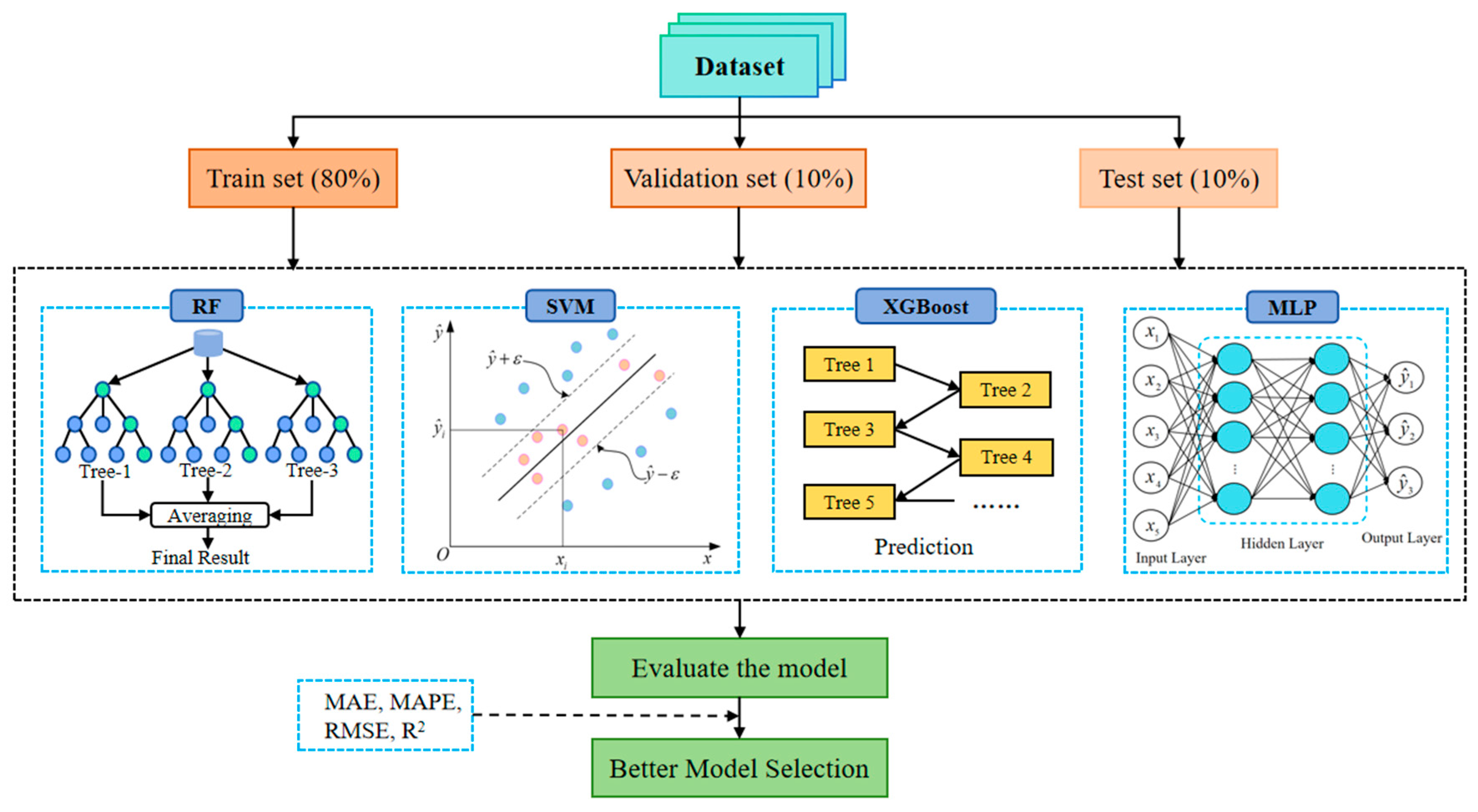
In summary, current methods for predicting external pressure fluctuations still face certain limitations in terms of rapid responses under multiple operational conditions and complex environmental scenarios, as well as in providing physical mechanism explanations. To address these issues, this paper proposes a machine learning prediction model that integrates optimization algorithms and explainability analysis methods. Firstly, a dataset of external pressure amplitude during high-speed train passage through tunnels was constructed using a numerical simulation. This dataset incorporates various typical operational conditions, including different tunnel lengths, train speeds, train lengths, blockage ratios, and measurement point positions. Subsequently, after completing data preprocessing, four representative machine learning models—random forest (RF), support vector regression (SVR), XGBoost, and Multilayer Perceptron (MLP)—were employed to model and predict external pressure fluctuation amplitudes. A systematic comparison of the models was conducted based on their prediction accuracy and generalization ability during the testing phase, leading to the selection of the best-performing model. Optimization algorithms were then applied to adaptively adjust the hyperparameters of this model, further enhancing its predictive performance. At the same time, a SHAP (SHapley Additive exPlanations) explainability analysis was integrated to quantitatively assess the contribution of different operational parameters to the pressure fluctuation amplitude predictions. This analysis helped identify the key features driving the predictions, providing data support and theoretical foundations for a subsequent aerodynamic characteristic analysis and the optimization design of tunnels.

2. Experimental Design

Given the limited data available in the existing literature regarding the external pressure amplitudes during the passage of a high-speed train through a tunnel, it is challenging to meet the demands for the high-quality sample data required for subsequent machine learning prediction models. To address this, this study employs Computational Fluid Dynamics (CFD) methods to numerically simulate the train operation process under typical conditions, thereby constructing a comprehensive and representative dataset. Through a controlled variable approach, simulation schemes are designed to systematically capture external pressure variation data under different combinations of tunnel and train parameters. This data will provide a solid foundation for subsequent model training and performance evaluation.

In this section, we will first introduce the governing equations, numerical calculation models, and boundary condition settings used in the simulations. The reliability and accuracy of the established models will be validated, and the process of dataset construction will be described in detail.

2.1. Governing Equations

The aerodynamic behavior of the train follows the fundamental fluid dynamics equations, which include the continuity equation, the momentum equation, and the energy equation. These governing equations describe the conservation of mass, momentum, and energy in the fluid flow around the train, forming the basis for the numerical simulation of the external pressure fluctuations during the train’s passage through the tunnel.

Continuity Equation (Conservation of Mass):

$${\displaystyle \frac{\partial \rho }{\partial t}}+{\displaystyle \frac{\partial }{\partial x_i}}\left(\rho u_i\right)=0$$

(1)

In the equation, t represents time; $u_i$ represents the component of the fluid velocity along the i-th direction, where i = 1, 2, 3 corresponds to the $x$, $y$, and $z$ directions, respectively.

Momentum Equation (Conservation of Momentum):

$${\displaystyle \frac{\partial }{\partial t}}\left(\rho u_i\right)+{\displaystyle \frac{\partial }{\partial x_j}}\left(\rho u_i{u}_j\right)=-{\displaystyle \frac{\partial p}{\partial x_i}}+{\displaystyle \frac{\partial {\tau }_{ij}}{\partial x_j}}+\rho g_i+F_i$$

(2)

In the equation, p denotes the static pressure, ${\tau }_{ij}$ represents the stress tensor, $g_i$ is the gravitational force component in the i-th direction, and $F_i$ denotes other energy terms arising from resistance and energy sources.

Energy Equation (Conservation of Energy):

$${\displaystyle \frac{\partial }{\partial t}}\left(\rho h\right)+{\displaystyle \frac{\partial }{\partial x_i}}\left(\rho u_{i}h\right)={\displaystyle \frac{\partial }{\partial x_i}}\left(k+k_t\right){\displaystyle \frac{\partial T}{\partial x_i}}+S_h$$

(3)

In the equation, h denotes the entropy, k represents the molecular conductivity, $k_t$ corresponds to the turbulent conductivity induced by turbulent transport, and $S_h$ denotes the volumetric source term.

In this study, we employed the SST k-ω turbulence model, which combines the advantages of the standard k-ε and k-ω models. The SST k-ω turbulence model adopts the standard k-ω formulation in the low Reynolds number regions near the train surface, while transitioning to the standard k-ε model in regions farther away from the wall. A blending function is employed to gradually shift from the wall-adjacent k-ω model to the outer k-ε model, thereby combining the advantages of both models. Due to its robustness and accuracy in capturing flow characteristics near walls and in the free stream, the SST k-ω model is widely used in engineering applications. Accordingly, this study adopts the SST k-ω turbulence model for the computational analysis of the high-speed train.

The transport equation for the turbulent kinetic energy k in the SST k-ω model is given as follows:

$${\displaystyle \frac{\partial \left(\rho k\right)}{\partial t}}+{\displaystyle \frac{\partial \left(\rho k{u}_i\right)}{\partial x_i}}={\displaystyle \frac{\partial }{\partial x_j}}\left({\Gamma }_k{\displaystyle \frac{\partial k}{\partial x_j}}\right)+G_k-Y_k+S_k$$

(4)

$${\displaystyle \frac{\partial \left(\rho \omega \right)}{\partial t}}+{\displaystyle \frac{\partial \left(\rho \omega u_i\right)}{\partial x_i}}={\displaystyle \frac{\partial }{\partial x_j}}\left({\Gamma }_{\omega }{\displaystyle \frac{\partial \omega }{\partial x_j}}\right)+G_{\omega }-Y_{\omega }+D_{\omega }+S_{\omega }$$

(5)

In the equation, $G_k$ represents the generation of turbulent kinetic energy; $G_{\omega }$ is the cross-diffusion term; ${\Gamma }_k$ and ${\Gamma }_{\omega }$ are the effective diffusivity terms for k and ω, respectively; $Y_k$ and $Y_{\omega }$ denote the dissipation terms of k and ω, respectively; and $S_k$ and $S_{\omega }$ are user-defined source terms.

2.2. Computational Model

According to relevant studies [27], a two-dimensional, revolving–axisymmetric train/tunnel model offers significant advantages in computational efficiency while maintaining a high level of accuracy comparable to that of three-dimensional simulations. Therefore, in this study, a two-dimensional, revolving–axisymmetric train/tunnel model is adopted to perform numerical simulations on a full-scale high-speed train. The SST $k-\omega$ is adopted to simulate the turbulent flow field, given its proven robustness and computational efficiency in predicting the aerodynamic characteristics of high-speed trains, and this is combined with an all-y⁺ wall treatment approach and an all-wall treatment approach to ensure the accurate capture of near-wall flow characteristics. The numerical simulations are performed using a finite volume method (FVM), with second-order spatial discretization schemes applied to enhance the solution accuracy. Temporal discretization is conducted using an implicit unsteady solver to ensure numerical stability during the simulation of transient pressure variations. The computational domain incorporates three types of boundary conditions: free-stream boundaries, wall boundaries, and overset mesh boundaries. Specifically, the tunnel walls and train surfaces are defined as wall boundaries, the region surrounding the train body is treated with overset mesh boundaries, and the remaining domain is designated as free-stream boundaries. At the free-stream boundaries, the inflow velocity is set according to the air velocity far away (e.g., 0 m/s), and the pressure is initialized at atmospheric conditions. Turbulence is specified using the intensity–length scale method, with a turbulence intensity of 5% and a length scale of 0.07 times the tunnel hydraulic diameter. The free-stream condition ensures realistic external flow behavior and avoids non-physical reflections. Combined with the overset mesh method, it enables the accurate simulation of the train’s movement and pressure wave propagation in the tunnel. 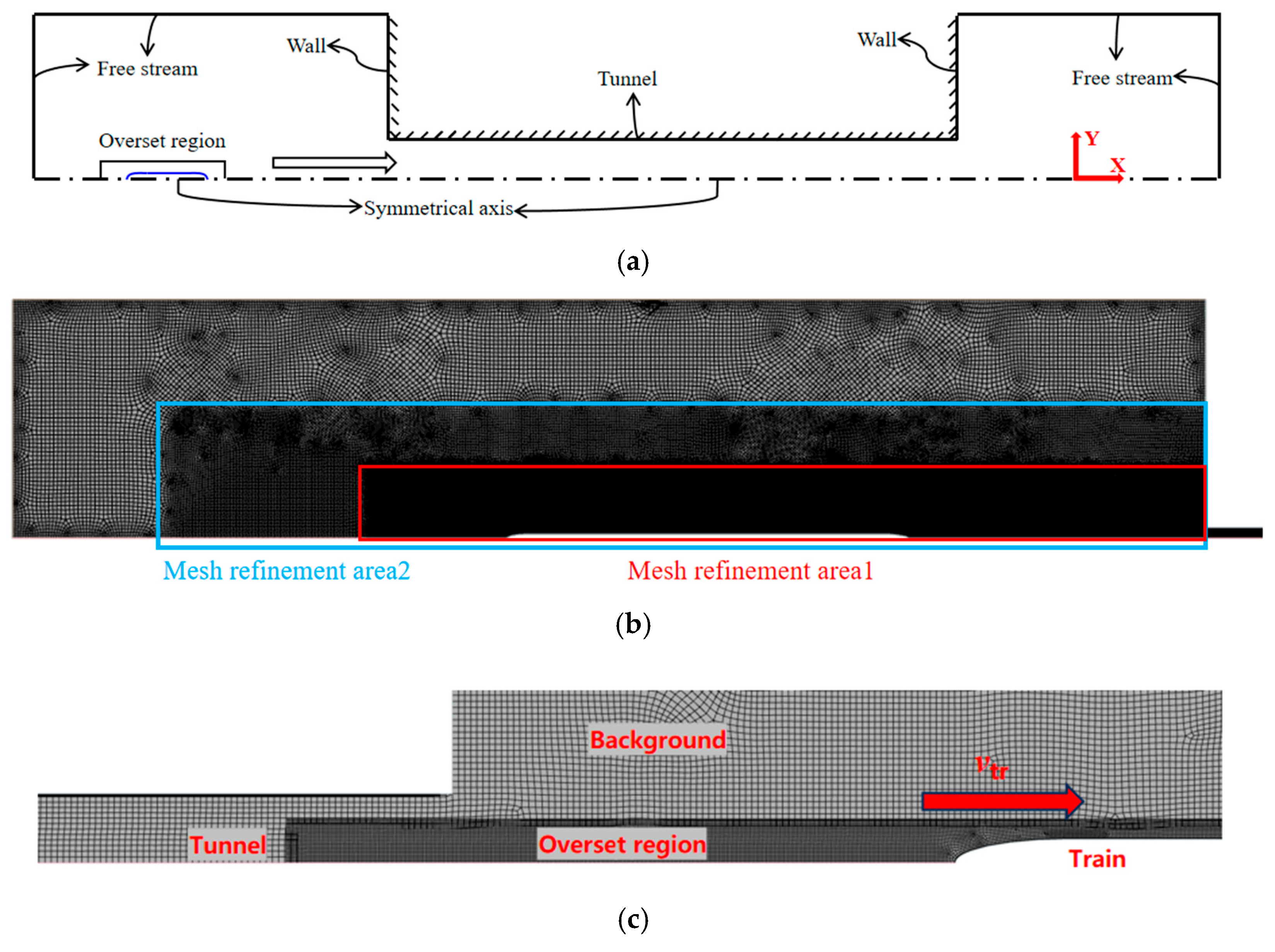The train model consists of eight carriages, with a total length of $L_{\mathrm{tr}}$ = 201.4 m, a cross-sectional area of $S_{\mathrm{tr}}$ = 11.85 m², and a body height of $L_{\mathrm{h}}$ = 3.7 m. Following industry standards, the computational domain is constructed as shown in Figure 1a to minimize boundary effects and ensure sufficient flow development. The computational domain height is set to 31.25 $L_{\mathrm{h}}$, with a distance of 600 $L_{\mathrm{h}}$ from the tunnel entrance to the upstream boundary and 300 $L_{\mathrm{h}}$ from the tunnel exit to the downstream boundary. This domain configuration effectively minimizes boundary-induced disturbances to the main flow region, thereby enhancing the accuracy and physical reliability of the simulation results.

A structured quadrilateral mesh was employed to discretize the entire computational domain, resulting in a total of approximately 206,000 cells. The mesh distribution of the computational domain is illustrated in Figure 1b. The first-layer thickness was set to 0.25 m, which corresponds to a dimensionless wall distance y+ > 30. This value places the first mesh point well within the log-law region, allowing for the use of wall function approaches in the SST k-ω turbulence model. We have adopted this mesh resolution intentionally to reduce the computational cost while maintaining acceptable accuracy, as our study focuses primarily on far-field external pressure wave propagation, rather than near-wall shear stress prediction. This strategy is commonly used in railway aerodynamics studies. To enhance the computational accuracy in critical regions, mesh refinement was applied around the train body and in areas with significant flow feature variations, ensuring the accuracy and stability of the numerical simulation results. Figure 1c shows the mesh layout around the train model. During the simulation, the overset mesh moves synchronously with the train in the positive velocity direction to accurately capture the dynamic evolution of the external flow field during the train’s motion.

Figure 2 illustrates the pressure–time histories obtained under different mesh densities. By comparing the simulation results using coarse (99,000 cells), medium (206,000 cells), and fine (438,000 cells) meshes, it is evident that the overall trends of the pressure curves remain consistent across all the mesh configurations, indicating a certain degree of stability in the simulation results concerning mesh resolution. Although the coarse mesh exhibits noticeable deviations in peak pressure compared to the medium and fine meshes, the medium mesh achieves a level of accuracy close to that of the fine mesh while significantly reducing the computational cost. Therefore, considering both accuracy and efficiency, the medium-density mesh is selected for subsequent simulations in this study.

2.3. Method Validation

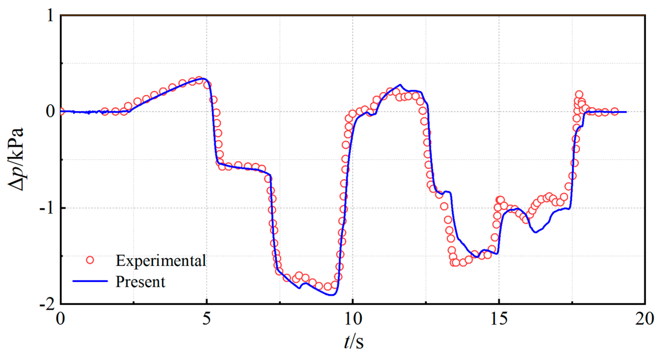
To verify the accuracy and applicability of the established numerical model, the full-scale experimental data of a high-speed train reported in Ref. [28] were selected for comparison. The test conditions were as follows: a train speed of 250 km/h, a tunnel length of 1080 m, and a tunnel cross-sectional area of 92 m². The pressure monitoring point was located on the train surface, 38 m from the train head. The pressure variations on the train surface during tunnel entry and passage obtained from the numerical simulation in this study were compared with the experimental measurements. The comparison results are shown in Figure 3. As shown in Figure 3, the numerical simulation results demonstrate a high degree of consistency with the experimental data in terms of the overall trend of pressure fluctuations, with the primary characteristic points closely matching.

Table 1. Error comparison of numerical calculation results.

Methods	Positive Pressure Peak/Pa	Negative Pressure Peak/Pa	Peak-to-Peak Pressure/Pa	Difference
Experimental	324.43	−1818.15	2142.58	—
Present	341.07	−1906.53	2247.60	4.9%

presents a comparison of errors between the numerical computation results. It is evident that the pressure amplitude obtained from the two-dimensional numerical calculation exhibits an error of 4.9% compared to the experimental pressure amplitude reported in the literature, which is within the reasonable error range of 10%. This indicates that the employed two-dimensional computational model demonstrates high predictive accuracy, providing strong support and reference for the subsequent construction of the external pressure dataset in tunnels.

2.4. Dataset Construction

During the process of a high-speed train traversing a tunnel, the external pressure fluctuations are influenced by a combination of factors. Previous studies have indicated that the structural form of the tunnel entrance significantly affects the pressure gradient, though its impact on the pressure amplitude is relatively limited [29]. Moreover, for high-speed trains with a streamlined design, the length of the train’s front section has a negligible effect on the pressure amplitude [30]. Given that the focus of this study is on a streamlined high-speed train and the variation in external pressure amplitude, the influence of the tunnel entrance structure and the train’s front length are disregarded in the experimental design to reduce variable interference and enhance the specificity of the analysis. This approach helps simplify the research model while emphasizing other key parameters that play a dominant role in pressure amplitude.

This study thoroughly considers five key factors influencing the external pressure fluctuations of a high-speed train as it passes through a tunnel during the experimental design phase. These factors include the tunnel length ($L_{\mathrm{tu}}$), train length ($L_{\mathrm{tr}}$), train speed ($v_{\mathrm{tr}}$), blockage ratio ($\beta$, defined as the ratio of the train cross-sectional area to the tunnel cross-sectional area), and the relative position of the measurement point ($x$). Based on two common train configurations, an 8-carriage train (train length = 200 m) and a 16-carriage train (train length = 400 m), a total of 2016 experiments were designed and completed. The specific initial conditions for the experiments are detailed in

Table 2. Initial experimental conditions.

Experiment No.	${\mathit{L}}_{\mathbf{tu}}/\mathbf{m}$	${\mathit{L}}_{\mathbf{tr}}/\mathbf{m}$	${\mathit{v}}_{\mathbf{tr}}/(\mathbf{km}\cdot {\mathbf{h}}^{-1})$	$\mathit{\beta }$
1	500	200	200	0.215
2	600	400	225	0.193
3	800		250	0.160
4	1500		275	0.140
5	2000		300	0.122
6	2500		320	0.112
7	3000		340
8	3500		350
	⋮
21	10,000

⋮ To maintain layout clarity and avoid redundancy, initial conditions with tunnel lengths increasing in 500 m increments from 3500 m to 10,000 m are collapsed. Only representative conditions are shown. Row 21 represents the final case with a tunnel length of 10,000 m.

. The tunnel length range was set from 500 m to 10,000 m; the train speeds covered typical operational ranges from 200 km/h to 350 km/h; the tunnel cross-sectional areas included common specifications, such as 52, 58, 70, 80, 92, and 100 m²; and the pressure measurement points are located at the midpoint on the exterior of each high-speed train carbody.

By combining different initial conditions for simulation, all results converged, yielding the external pressure amplitude dataset. A portion of the dataset is presented in

Table 3. Pressure amplitude data (partial).

No.	${\mathit{L}}_{\mathbf{tu}}/\mathbf{m}$	${\mathit{L}}_{\mathbf{tr}}/\mathbf{m}$	${\mathit{v}}_{\mathbf{tr}}/(\mathbf{km}\cdot {\mathbf{h}}^{-1})$	$\mathit{\beta }$	$\mathit{x}/\mathbf{m}$	${\mathit{P}}_{\mathbf{max}}/\mathbf{kPa}$	${\mathit{P}}_{\mathbf{min}}/\mathbf{kPa}$	$\mathbf{\Delta }\mathit{P}/\mathbf{kPa}$
1	1500	200	200	0.112	0.0625	0.248	−1.095	1.343
2	1500	200	200	0.122	0.0625	0.288	−1.195	1.483
3	1500	200	200	0.140	0.0625	0.360	−1.372	1.732
⋮	⋮	⋮	⋮	⋮	⋮	⋮	⋮	⋮
24,191	10,000	400	350	0.193	0.9688	0.820	−5.555	6.375
24,192	10,000	400	350	0.215	0.9688	0.993	−7.684	8.677

⋮ To maintain clarity and avoid redundancy, only partial pressure amplitude data are presented. The row numbers indicate that the intermediate data (from No. 4 to No. 24,190) are omitted.

. The dataset was derived based on the governing equations of fluid dynamics used in the numerical model, which describe the conservation of mass, momentum, and energy in the flow field, as shown in Equations (1)–(5). These equations were solved numerically using the finite volume method implemented in STAR-CCM+. The input features for the predictive model include the following five parameters: tunnel length ($L_{\mathrm{tu}}$), train length ($L_{\mathrm{tr}}$), train speed ($v_{\mathrm{tr}}$), blockage ratio ($\beta$), and measurement point location ($x$). The output consists of multiple target variables, including the positive peak value ($P_{\max }$), negative peak value ($P_{\min }$), and peak-to-peak value ($\Delta P$, the difference between the positive and negative peaks), which comprehensively reflect the characteristics of external pressure variation as the train enters the tunnel.

3. Data Processing and Analysis

3.1. Data Preprocessing

Due to the differences in dimensions and value ranges among the input features in the original dataset, directly utilizing these features for modeling may cause those with larger magnitudes to dominate the training process. This imbalance could adversely affect the regression outcomes, reducing the model’s stability and generalization capability. To mitigate the interference caused by scale discrepancies among features, it is necessary to perform feature standardization prior to training. Standardization transforms each feature into a common numerical range, typically reshaping their distribution toward a standard normal form (a mean of 0 and a standard deviation of 1). This procedure enhances convergence efficiency, accelerates the training process, and improves the overall stability and robustness of the model. Based on these considerations, standardization was applied prior to model training in this study. The calculation formula is as follows:

$$X^{\prime }={\displaystyle \frac{X-\mu }{\sigma }}$$

(6)

where $X$ denotes the original data, $X^{\prime }$ represents the standardized data, $\mu$ is the mean, $\sigma$ and is the standard deviation.

To ensure comparability across features with varying units and magnitudes, normalization is performed using the method described in Equation (6). This step is essential for improving model convergence and prediction stability.

3.2. Correlation Analysis

During the data modeling process, the correlation between different features plays a crucial role in model performance. Highly correlated features can lead to multicollinearity, which negatively impacts the robustness of the model, while irrelevant or weakly correlated features may contribute little to the prediction, increasing the model complexity. Therefore, in the feature engineering phase, it is essential to perform a correlation analysis to select key variables and enhance the model’s generalization ability. A commonly used method is the Pearson correlation coefficient, which measures the degree of linear correlation between two variables.

Assuming there are m objects and n indicators, the data matrix is denoted as $X={\left(x_{ij}\right)}_{\mathrm{m}\times \mathrm{n}}$. If we are interested in the correlation between the a-th column, $x_a$, and the b-th column, $x_b$, of the data matrix, let the correlation coefficient between columns a and b be denoted as Pearson’s r(a, b); then,

$$r\left(a,b\right)={\displaystyle \frac{{\displaystyle \sum _{i=1}^m\left(x_{a,i}-{\overline{x}}_a\right)\left(x_{b,i}-{\overline{x}}_b\right)}}{\sqrt{{\displaystyle \sum _{i=1}^m{\left(x_{a,i}-{\overline{x}}_a\right)}^2}}\sqrt{{\displaystyle \sum _{j=1}^m{\left(x_{b,j}-{\overline{x}}_b\right)}^2}}}}$$

(7)

In the equation, ${\overline{x}}_a$ and ${\overline{x}}_b$ represent the means of $x_a$ and $x_b$, respectively; $\left(x_{a,i}-{\overline{x}}_a\right)$ $\left(x_{b,i}-{\overline{x}}_b\right)$ denotes the product of the deviations of variables $x_a$ and $x_b$ at the i-th observation.

The Pearson correlation coefficient ranges from [−1, 1], where values closer to 1 indicate a strong positive linear relationship between variables, values closer to −1 suggest a strong negative linear relationship, and values near 0 imply little to no linear association between the variables. Based on the correlation coefficient formula defined in Equation (7), Figure 4 presents the correlation matrix, illustrating the relationships among all variables. A pie chart representation is used to intuitively convey both the strength and direction of pairwise correlations. Each label (e.g.,$L_{\mathrm{tu}}$,$L_{\mathrm{tr}}$,$v_{\mathrm{tr}}$) denotes a specific variable. The color of each pie segment indicates the direction of the correlation—blue signifies a positive relationship, while red denotes a negative one. The filled area of each pie reflects the absolute value of the Pearson correlation coefficient; the closer the value is to 1, regardless of sign, the stronger the linear association. Moreover, asterisks are used to mark statistical significance, * for p < 0.05, ** for p < 0.01, and *** for p < 0.001, facilitating the assessment of the reliability of each correlation.

As illustrated in Figure 4, the input variables $v_{\mathrm{tr}}$ and $\beta$ exhibit strong correlations with the output variables $P_{\max }$,$P_{\min }$, and $\Delta P$. In contrast, other input variables demonstrate relatively weak influence within the current model, and there is no significant intercorrelation among the input features. Despite the weak linear correlation between the tunnel length (L_tu) and the target variables, this parameter was retained in the input set due to its physical relevance in the formation and propagation of tunnel pressure waves. It may also contribute to prediction performance through nonlinear interactions, which are not captured by linear correlation metrics. These findings provide a valuable reference for subsequent feature selection and model development. Guided by the correlation analysis, the selection of input variables can be further optimized to enhance both the predictive accuracy and the stability of the regression model.

4. Methods

4.1. Machine Learning Model

In regression tasks, machine learning models are generally categorized into linear regression, tree-based models, support vector regression, and neural networks. Given the pronounced nonlinear relationship between the external pressure amplitude and input variables, this study selects representative algorithms with strong nonlinear modeling capabilities from these categories—namely, random forest regression (RF), support vector regression (SVR), Extreme Gradient Boosting (XGBoost), and Multilayer Perceptron (MLP)—to construct predictive models for pressure amplitude. To ensure effective training and fair evaluation, the dataset is randomly partitioned: 80% is used for training, 10% for validation to optimize hyperparameters, and the remaining 10% for testing the generalization performance of the models. This split enhances the training stability and ensures predictive reliability on unseen data. The modeling procedures for the four algorithms are illustrated in Figure 5. All the machine learning models were developed and evaluated using MATLAB R2023b’s built-in toolboxes, which provide robust functions for training, validating, and comparing regression algorithms. By comparing their predictive performance on the same dataset, this study systematically evaluates the accuracy differences across models, thereby identifying the most suitable regression approach for the given task. The results provide a theoretical foundation and methodological reference for subsequent model optimization and practical application. The theoretical basis for the four regression models (random forest, support vector regression, MLP, and XGBoost) is presented in Equations (8) and (9). These formulations are critical for constructing and training the models discussed in Section 5.1. The following subsections briefly introduce the core principles of each model.

4.1.1. Random Forest Regression (RF)

Random forest is an ensemble learning model based on decision trees, which enhances predictive performance by aggregating the outputs of multiple individual trees [31]. The procedure of the random forest algorithm can be summarized as follows:

• During training, the random forest employs a bootstrap sampling strategy, wherein N samples are randomly drawn with replacement from the original training dataset to generate multiple training subsets. Each subset is used to independently train a distinct decision tree.
  If the original dataset is denoted as $D=\{\left(x_1,y_1\right),\left(x_2,y_2\right),\cdots ,\left(x_N,y_N\right)\}$, then the K-th training subset is represented as $D_k=\{\left(x_{1k},y_{1k}\right),\left(x_{2k},y_{2k}\right)\cdots \left(x_{Nk},y_{Nk}\right)\}$, where $x_i$ denotes the input features, and $y_i$ denotes the corresponding target variable.
• When constructing each decision tree, the selection of the splitting feature at each node is not based on the entire set of M features. Instead, a subset of m features is randomly selected from the full feature set, and the optimal feature is chosen from this subset for node splitting. This dual-randomization strategy—applied to both samples and features—introduces diversity among individual trees, thereby reducing the risk of overfitting and enhancing the model’s generalization capability.
• The final prediction of the random forest model is obtained by averaging the predictions of all decision trees in the ensemble, which can be expressed as follows:

  $$\widehat{y}={\displaystyle \frac{1}{K}}{\displaystyle \sum _{k=1}^K{h}_k\left(x\right)}$$

  (8)

In the equation, $\widehat{y}$ denotes the final predicted value; K represents the total number of decision trees in the random forest; and $h_k\left(x\right)$ indicates the prediction output of the k-th decision tree.

In this study, the number of decision trees and the minimum number of leaf nodes were optimized within the bounds LB [10, 1] and UB [200, 5], respectively. The model was tuned to strike a balance between prediction accuracy and computational efficiency.

4.1.2. Support Vector Regression (SVR)

Support vector regression (SVR) is a regression technique derived from Support Vector Machines (SVM) [32]. The objective of SVR is to find a linear function f(x) that approximates the target values, y, while minimizing the prediction error. The core principle involves constructing a hyperplane to represent the regression function. The hyperplane expression is $f\left(x\right)={\omega }^{T}x+b$. To effectively handle nonlinear relationships, SVR employs kernel functions to map the input data into a high-dimensional feature space. The choice of kernel, such as linear, polynomial, or radial basis function (RBF), depends on the underlying characteristics and the complexity of the data. During training, SVR introduces an ε-insensitive loss function, typically within the range [−ε, ε], where errors falling within this interval are not penalized. This approach enhances the model’s generalization ability by focusing on significant deviations from the predicted values.

The SVM model was optimized using three hyperparameters: BoxConstraint(C), KernelScale, and Epsilon (insensitive loss parameter). Specifically, BoxConstraint represents the box constraint, C, on the alpha coefficients; KernelScale is the kernel function value; and Epsilon is half of the insensitive bandwidth(ε). The search bounds were LB [0.01, 0.01, 0.001] and UB [5, 30, 1]. These parameters were tuned to enhance the generalization performance while preserving model robustness.

4.1.3. Extreme Gradient Boosting (XGBoost)

Extreme Gradient Boosting (XGBoost) is an optimized gradient boosting algorithm that integrates multiple weak learners (typically decision trees) into a strong predictive model [33]. Each tree is trained to minimize the residuals (i.e., prediction errors) from the previous iteration, thereby progressively refining the model’s accuracy. The algorithm employs a gradient boosting framework, leveraging both the first- and second-order derivatives of the loss function to update tree weights and guide the model toward a global optimum.

During the tree construction process, XGBoost adopts a greedy algorithm to select the most informative features for node splitting. Candidate split points are evaluated based on information gain, and the feature that yields the greatest gain is prioritized. Moreover, the objective function in XGBoost comprises both a loss term and a regularization term. By minimizing this objective, the algorithm balances model accuracy and complexity, effectively reducing the risk of overfitting while enhancing predictive performance.

In this study, the maximum number of iterations, maximum tree depth, and minimum child weight were selected as key hyperparameters. The corresponding optimization ranges were iter_range = [10, 300], depth_range = [1, 10], and min_child_range = [1, 10]. These were adjusted to control overfitting and improve the prediction accuracy.

4.1.4. Multilayer Perceptron (MLP)

Multilayer Perceptron (MLP) is a representative type of feedforward neural network, typically comprising an input layer, one or more hidden layers, and an output layer [34]. In this study, the MLP model is trained using the Levenberg–Marquardt (LM) algorithm, which integrates the advantages of both the gradient descent and the Newton method, making it particularly effective for nonlinear optimization tasks. The LM algorithm dynamically adjusts the parameter Mu to switch between the gradient descent (when Mu is large) and the Newton method (when Mu is small), thereby accelerating convergence and enhancing the training stability.

The core structure of MLP is based on a fully connected network, and feature extraction is achieved through weight mapping between layers and parameter optimization of the back propagation algorithm. With the help of optimization strategies, such as gradient descent, the weights and biases in the network are continuously adjusted to minimize the loss function and improve the prediction accuracy of the model. The computational process of MLP completes the feature transformation through the weighted summation of the neurons in each layer and the mapping of activation functions. For k neurons in the output layer, the output value is expressed by the following equation:

$${\widehat{y}}_k={\displaystyle \sum _{i=1}^n{\omega }_i{x}_i+b_i}$$

(9)

where ${\omega }_i$ denotes the weight connecting hidden layer neurons to the output layer neuron; $b_i$ is the bias term; and ${\widehat{y}}_k$ represents the final predicted value.

In this study, the MLP model was constructed using a regularization-based loss function (MSE with L2 penalty). The hyperparameters optimized included the regularization coefficient (Lambda) and the architecture of the network (LayerSizes). The search bounds were LB [1, 2, 2, 0.001] and UB [3, 50, 50, 0.3]. Here, the LayerSizes represent the number of hidden layers and the number of neurons in each layer.

4.2. Evaluation Metrics

To evaluate the predictive performance of the regression models, four evaluation metrics were employed: the Mean Absolute Error (MAE), Mean Absolute Percentage Error (MAPE), Root Mean Square Error (RMSE), and the coefficient of determination (R²) [35]. The corresponding mathematical expressions are presented in Equations (10)–(13). A lower MAE, MAPE, and RMSE, along with a higher R² value, indicates a better model performance. The corresponding mathematical expressions are as follows:

$$MAE={\displaystyle \frac{1}{n}}{\displaystyle \sum _{i=1}^n\left|y_i-{\hat{y}}_i\right|}$$

(10)

$$MAPE={\displaystyle \frac{1}{n}}{\displaystyle \sum _{i=1}^n\left|\frac{y_i-{\hat{y}}_i}{y_i}\right|}\times 100\%$$

(11)

$$RMSE=\sqrt{{\displaystyle \frac{1}{n}}{\displaystyle \sum _{i=1}^n{\left(y_i-{\widehat{y}}_i\right)}^2}}$$

(12)

$$R^2=1-{\displaystyle \frac{{\displaystyle \sum _{i=1}^n{\left(y_i-{\widehat{y}}_i\right)}^2}}{{\displaystyle \sum _{i=1}^n{\left(y_i-{\overline{y}}_i\right)}^2}}}$$

(13)

In the equation, $y_i$ denotes the true value of the pressure amplitude (kPa), ${\widehat{y}}_i$ represents the predicted value of the pressure amplitude (kPa), and $\overline{y}$ is the mean value of the pressure amplitude (kPa).

4.3. Hyperparameter Optimization Strategy

Optimization algorithms represent a class of heuristic-based search techniques designed to fine-tune model hyperparameters [36]. The fundamental principle involves iteratively applying optimization strategies to explore the global optimum, thereby enhancing the convergence efficiency and the solution accuracy. Given an optimization problem defined as $\mathit{min}F\left(x\right),x\in \mathsf{\Omega }$, where $F\left(x\right)$ is the objective function, $x$ denotes the decision variables, and $\mathsf{\Omega }$ represents the feasible solution space, the process begins with a randomly initialized population $P=\{x_1,x_2,\cdots ,x_N\}$ within the solution space, where N is the population size. The objective function value $F\left(x_i\right)$ is obtained by evaluating the fitness of each individual $x_i\left(i=1,2,\cdots ,N\right)$. For minimization problems, a smaller fitness value indicates better individual performance. Based on the specific strategy of the optimization algorithm, the positions of individuals in the population are updated accordingly. For instance, in Particle Swarm Optimization (PSO), the position update of each particle is governed by the following equations:

$$v_i^{t+1}=\omega v_i^t+c_1{r}_1\left(p_i^t-x_i^t\right)+c_2{r}_2\left(g^t-x_i^t\right)$$

(14)

$$x_i^{t+1}=x_i^t+v_i^{t+1}$$

(15)

In the equation, $v_i^t$ and $x_i^t$ represent the velocity and position of the i-th individual in the t-th generation, respectively; $p_i^t$ denotes the individual’s personal best solution; $g^t$ is the global best solution; $\omega$ is the inertia weight; $c_1$ and $c_2$ are the learning factors; and $r_1$ and $r_2$ are random numbers within the range [0, 1].

If the change in the objective function is smaller than a specified threshold or the maximum number of iterations is reached, the current best solution, $x^{*}$, and its corresponding objective function value, $F\left(x^{*}\right)$, are returned.

4.4. Shapley Additive exPlanations (SHAP)

SHAP [37,38] is a method used to explain the outputs of any machine learning model. It is derived from the concept of Shapley values in game theory [39]. SHAP evaluates the importance of a given feature by computing the sum of its marginal contributions across all the possible feature permutations.

Specifically, the SHAP value of a particular feature, $X_i$, in a model represents its contribution to the prediction result, and is defined as follows:

$${\varphi }_i={\displaystyle \sum _{S\subseteq N\backslash \{i\}}\frac{\left|S\right|!\left(\left|N\right|-\left|S\right|-1\right)!}{\left|N\right|!}}-\left[f\left(S\cup \{i\}\right)-f\left(S\right)\right]$$

(16)

In this equation, N represents the set of all the features; S denotes a subset of features, excluding feature i; $f\left(S\right)$ is the model’s prediction under the feature subset S; and ${\varphi }_i$ is the SHAP value of feature $X_i$.

In this study, a SHAP analysis was performed in the MATLAB environment using customized functions to compute and visualize the feature contributions. This method enables a fair and interpretable quantification of each feature’s individual contribution and importance to the model prediction and has been widely applied in the interpretability analyses of complex models.

5. Results

5.1. Model Performance

To reduce the risk of model overfitting and enhance the model’s generalization capability, this study incorporates an L² regularization strategy during model training. L² regularization introduces a penalty term—the sum of squared weight parameters—into the loss function, which suppresses excessively large weights and prevents the model from over-relying on a small number of features. During the feature selection phase, L² regularization promotes a more balanced distribution of weights, enabling the model to fully exploit the available feature information, thereby improving its robustness and generalization performance.

Given the varying suitability of different machine learning models, this study evaluates the performance of four representative models—random forest (RF), support vector regression (SVR), XGBoost, and Multilayer Perceptron (MLP)—in predicting external pressure. The models’ predictive performances are quantitatively compared on the training, validation, and test datasets, with the results illustrated in Figure 6.

As shown in the figure, the random forest model exhibits noticeably lower errors on the training set compared to the validation and test sets, indicating a certain degree of overfitting during training. Although RF fits the training data well, its generalization ability is limited. Moreover, the relatively low coefficient of determination (R²) on the test set further reflects its lack of robustness. Therefore, the random forest model is not considered the optimal choice for this task.

The SVM model exhibits similar error levels across the training, validation, and test sets, indicating the absence of overfitting, as the training error is not significantly lower than the validation error. However, the overall prediction error remains relatively high, suggesting that the model struggles to accurately capture the nonlinear relationships between the input parameters and the external pressure amplitude. Consequently, SVM is not well-suited for the current prediction task.

The XGBoost model demonstrates a balanced distribution of errors across the training, validation, and test sets, reflecting its strong generalization ability. Nonetheless, its overall error is slightly higher than that of the MLP model, indicating that its predictive performance for the external pressure amplitude is somewhat inferior to that of MLP.

Although the RMSE value of the MLP model on the test set is slightly higher compared to XGBoost and RF, its performance in terms of the MAE and the MAPE remains the best, and it also achieves the highest R² score. Considering that the RMSE is more sensitive to outliers, the higher RMSE value may be attributed to a few extreme cases, while the overall error distribution remains low and stable. Thus, the MLP model is considered more robust and generalizable for this task.

In summary, the MLP model outperforms the other methods in terms of prediction accuracy in this study. However, its stability and precision under complex operating conditions still have room for improvement. To enhance the model’s robustness and predictive performance across diverse scenarios, future work will consider the integration of intelligent optimization algorithms.

5.2. Comparison of MLP Model Performance Before and After Hyperparameter Optimization

To further improve the prediction accuracy and generalization capability of the MLP model, this study introduces intelligent optimization algorithms to enhance both its architecture and hyperparameter settings. Specifically, adaptive optimization techniques, such as the sparrow search algorithm (SSA) [40], Simulated Annealing (SA) [41], Particle Swarm Optimization (PSO) [42], the Snake Optimization Algorithm (SOA) [43], and the Sine–Cosine Algorithm (SCA) [44] are employed to automatically tune key hyperparameters, including the number of hidden layers, the number of neurons per layer, and the regularization coefficient. This approach aims to mitigate the limitations of manual parameter tuning, accelerate convergence, and improve the overall stability of the model. The optimization workflow of MLP using intelligent algorithms is illustrated in Figure 7.

During the optimization process, an early stopping mechanism is introduced to prevent overfitting. In addition, the Levenberg–Marquardt algorithm is employed for weight updates, with the Mu parameter dynamically adjusted during training to enhance the optimization performance. The hyperparameter search space is defined as follows: the learning rate is set within the range of [0.0001, 0.1], and the number of neurons in the hidden layer is selected from [10, 200]. The mean squared error (MSE) is used as the fitness function to guide the model’s training and optimization.

The optimized MLP model with the improved optimization algorithm is compared with the unoptimized MLP model, and the performance is evaluated using various metrics. Figure 8 illustrates the prediction performance of six different models on the test set, where the horizontal axis represents the true data values, and the vertical axis represents the model’s predicted values. The color of the data points indicates the density distribution, with high-density areas shown in red and low-density areas in blue. From Figure 8, it can be observed in subplot (b) that most of the data points are tightly clustered near the ideal diagonal line, indicating that the SSA-MLP model achieves a higher predictive accuracy. The slope of the regression fit line is close to one, and the intercept is small, reflecting a low overall bias. Additionally, the correlation coefficient of this model is higher than that of other models, further confirming its stability and generalization ability on the test set. Overall, SSA-MLP outperforms other methods in accurately capturing the variation trend of the true data, with predictions showing a higher degree of alignment with the true values. Therefore, this method demonstrates superior performance in this task, providing an effective optimization strategy to enhance the predictive capability of the MLP model.

Table 4. Comparison of evaluation metrics for the optimized MLP model.

Model	R2			RMSE			MAPE
	Training Set	Validation Set	Test Set	Training Set	Validation Set	Test Set	Training Set	Validation Set	Test Set
MLP	0.999	0.976	0.880	0.028	0.186	0.411	0.012	0.041	0.085
SSA-MLP	0.999	0.996	0.993	0.050	0.084	0.112	0.018	0.038	0.052
SA-MLP	0.999	0.998	0.989	0.015	0.068	0.135	0.007	0.023	0.063
PSO-MLP	0.988	0.976	0.974	0.132	0.205	0.213	0.042	0.070	0.099
SOA-MLP	0.997	0.993	0.984	0.066	0.119	0.169	0.021	0.046	0.075
SCA-MLP	0.999	0.995	0.982	0.015	0.089	0.179	0.007	0.027	0.083

shows the comparison of the R², RMSE, and MAPE metrics for the MLP model with different optimization algorithms on the training set, validation set, and test set. As shown in Table 4, the R² of the MLP model reaches 0.999 on the training set, indicating an extremely high fit. However, the R² drops to 0.880 on the test set, suggesting that the model may suffer from overfitting. The RMSE is 0.028 on the training set, but increases to 0.411 on the test set, further demonstrating the model’s lack of generalization ability. The MAPE is 0.012 on the training set, but rises to 0.085 on the test set, indicating a substantial error in the unseen data.

The SSA-MLP model achieves an R² of greater than 0.99 across all the datasets, with a notable improvement on the test set, where the R² increases to 0.993: a 12.8% increase compared to the MLP model. The RMSE drops to 0.112, a 72.7% decrease, and the MAPE decreases to 0.052, a 38.8% reduction, significantly enhancing the model’s generalization ability. The SA-MLP model achieves an R² of 0.989 on the test set, with an RMSE of 0.135 and a MAPE of 0.063. While these metrics are slightly lower than those of SSA-MLP, they still outperform the original MLP model. The PSO-MLP model has an R² of 0.988 on the training set, slightly lower than the original MLP, but the R² on the test set improves to 0.974. However, the RMSE (0.213) and the MAPE (0.099) on the test set are noticeably higher than those of SA-MLP and SSA-MLP, suggesting that the optimization effect is relatively limited, possibly due to convergence to a local optimum. The SOA-MLP model performs well on the test set, with an R² of 0.984, an RMSE of 0.169, and a MAPE of 0.075, showing improvements over PSO-MLP, though its metrics are still slightly lower than those of SSA-MLP. The SCA-MLP model achieves an R² of 0.982, an RMSE of 0.179, and a MAPE of 0.083 on the test set, performing slightly worse than SOA-MLP, but still outperforming the original MLP model.

In conclusion, the SSA-MLP model outperforms all the other models across all the metrics, demonstrating a strong generalization ability and effectively reducing the test error. The SA-MLP model follows closely, particularly excelling in the MAPE, showcasing its robust generalization capability. The PSO-MLP, SOA-MLP, and SCA-MLP models all show improvements over the original MLP, but their optimization effects are not as effective as those of SSA-MLP and SA-MLP. Therefore, MLP models optimized with algorithms like SSA and SA can effectively mitigate overfitting, enhance the generalization ability, and maintain a high prediction accuracy on the test set.

5.3. Model Interpretation

To enhance the model’s interpretability, the SHAP method is employed, grounded in cooperative game theory. Its mathematical basis is detailed in Equation (16), which underpins the analysis results shown in this section. To further explore the influence of each input feature on the SSA-MLP model’s prediction of the external pressure amplitude, SHAP values are used for the interpretability analysis of the model results, as shown in Figure 9. The horizontal axis represents the input features, while the vertical axis shows the SHAP values, reflecting the contribution of each feature to the model output. A larger SHAP value indicates a greater positive contribution of the feature to the prediction, whereas a smaller SHAP value represents a negative contribution. The color of the points indicates the feature’s value, with red representing higher values and blue representing lower values.

As shown in Figure 9, for the positive peak value, $P_{\max }$, the SHAP value distribution reveals that the relative measurement position, x, and the blockage ratio, $\beta$, have the most significant influences on the prediction results. High feature values are primarily distributed in the region with positive SHAP values, indicating that an increase in these features substantially enhances the predicted value. Train speed, $v_{\mathrm{tr}}$, also exhibits a strong impact; its SHAP values tend to be positive as the speed increases, suggesting that higher speeds contribute more to the prediction of the $P_{\max }$. The influence of train length, $L_{\mathrm{tr}}$, is moderate, with SHAP values distributed around zero and showing a balanced mix of positive and negative contributions. Tunnel length, $L_{\mathrm{tu}}$, has the weakest impact, with the SHAP values highly concentrated near zero and exhibiting minimal fluctuation, indicating a limited contribution to the prediction of the $P_{\max }$. In summary, the relative measurement position, blockage ratio, and train speed are the dominant factors influencing the prediction of the $P_{\max }$, while the effects of train length and tunnel length are comparatively weaker.

For the negative peak value, $P_{\min }$, train speed, $v_{\mathrm{tr}}$, is the most influential factor, as evidenced by the widest SHAP value distribution. High feature values are mainly associated with negative SHAP values, indicating that a higher train speed corresponds to a larger negative peak amplitude. The blockage ratio ranks second in importance and exhibits a similar trend—larger blockage ratios result in greater negative peak amplitudes. The SHAP values for the relative measurement position are concentrated around zero, suggesting a limited contribution to the prediction. Similarly, the effects of tunnel length and train length are minimal, as indicated by the narrow and centered SHAP distributions. These results demonstrate that train speed and the blockage ratio are the primary factors influencing the prediction of the negative peak value, while the impact of other features is relatively weak.

For the peak-to-peak value, $\Delta P$, the SHAP value distribution indicates that train speed, $v_{\mathrm{tr}}$, is the most influential factor. It exhibits the widest SHAP value range, with higher speeds corresponding to positive SHAP values, suggesting that greater speeds lead to larger $\Delta P$ values. The blockage ratio, $\beta$, is the second-most important factor, showing that the $\Delta P$ increases with the increasing blockage ratio. Tunnel length, $L_{\mathrm{tu}}$, ranks next in importance, where longer tunnels are generally associated with negative SHAP values, implying that the $\Delta P$ decreases as the tunnel length increases—possibly due to the attenuation effect of pressure wave propagation. In contrast, train length, $L_{\mathrm{tr}}$, and the relative measurement position, $x$, have SHAP values concentrated around zero, indicating their limited contribution to the prediction of the $\Delta P$. These results demonstrate that train speed and the blockage ratio are the primary factors affecting the prediction of the $\Delta P$, followed by tunnel length, while train length and the measurement position have relatively minor impacts.

In summary, train speed and the blockage ratio are identified as the core features influencing the prediction of the external pressure amplitude, while the importance of other features varies depending on the specific prediction target. This conclusion provides a theoretical basis for feature selection and model optimization and further validates the physical consistency and reliability of the SSA-MLP model. The SHAP analysis not only enhances interpretability but also provides actionable engineering insights. For instance, the identification of key influencing factors can guide tunnel and train designers in prioritizing parameters during the early stages of design and optimization. Furthermore, understanding the marginal effects of each input variable supports data-driven decisions in model refinement, contributing to both accuracy and robustness. It is worth noting that although tunnel length exhibits relatively low importance in the SHAP analysis, it was deliberately retained as an input variable. This decision is grounded in its physical relevance to the development and propagation of pressure waves, especially in scenarios involving long tunnels. While its marginal contribution to prediction accuracy may be limited under certain conditions, excluding such a physically meaningful parameter could compromise the model’s generalizability across broader engineering contexts.

6. Conclusions

Based on the findings, this study proposes a hybrid modeling strategy that integrates numerical simulations with machine learning. While CFD provides high-fidelity pressure amplitude data, its high computational cost limits large-scale scenario exploration. To address this, an SSA-MLP model was trained on CFD-generated data under varying tunnel lengths, train speeds, and blockage ratios, enabling fast and reliable pressure predictions across multiple conditions. To improve the model’s transparency, a SHAP analysis was used to quantify the influence of each input. The results show that train speed and the blockage ratio are the most influential factors, followed by tunnel length and measurement position; train length has a minimal effect. These insights support future integrated tunnel–train design and operational optimization.

Several limitations are acknowledged. This study uses a 2D, axisymmetric CFD model, which omits 3D effects, such as crosswinds and lateral flows. Future work should explore full 3D simulations for enhanced accuracy. Additionally, due to time and space constraints, statistical significance testing (e.g., confidence intervals) was not included. Such analyses would strengthen the performance validation and are planned for future studies. Moreover, fixed train nose and tunnel entrance profiles were adopted based on standard references to reduce complexity. While prior studies suggest nose geometry may have a limited impact under certain conditions, this assumption requires further validation. Future work should incorporate a sensitivity analysis of geometric parameters to enhance the model’s generalizability.

Despite these limitations, the hybrid simulation–ML framework developed herein demonstrates a strong potential for practical engineering applications. It can serve as an efficient surrogate model, enabling the rapid evaluation of pressure wave impacts under diverse operational conditions and supporting iterative design and scenario-based assessments for tunnel and rolling stock engineers.