Abstract
In this paper, multi-option probabilistic paired comparison models are presented and applied for prediction. As these models operate on the basis of probabilities, they can estimate the likelihood of future outcomes and thus predict future events. The aim of the paper is to demonstrate that these models have strong predictive capabilities when the information embedded into the data is properly utilized. To this end, we incorporate the degree (e.g., large or small) of the differences between the compared objects. By refining the usual three-option model, we define a five-option model capable of leveraging information derived from the goal differences. To incorporate additional information, the model is further extended to account for potential advantages in the comparisons. As a further refinement, temporal weighting is also introduced. These models are applied to forecasting football match outcomes in the top five European leagues (Premier League, La Liga, Serie A, Bundesliga, and Ligue 1), and their predictive performance is evaluated using various metrics. Based on the most recent football seasons, this model consistently delivers better predictive metrics, on average, than those of the already strong benchmark model. The effect of a home-field advantage is statistically supported across all five leagues. The model fits are illustrated using confidence intervals, and, as an interesting insight, we also present the evolution of the team strengths for the top four English clubs during the 2023/24 season.
1. Introduction
Predicting future events, assessing them, and preparing accordingly have always been important. This applies to environmental and societal changes, market trends, and even the outcomes of sporting events and team performances. The more significantly an upcoming event affects us, the more beneficial it is to be well prepared. In most cases, there are numerous possible future outcomes, and it is often impossible to prepare for all of them, especially when some are mutually exclusive. Therefore, it is crucial to allocate resources toward outcomes that are more likely to occur. By predicting future events, we can better identify which scenarios are worth preparing for. By assessing the likelihood of various outcomes, we can focus on what is most probable.
Different areas of forecasting require different methods. Specialized models are developed for economic problems [1,2], weather forecasting [3,4], and the outcomes of sport events [5,6], but in every case, data are needed, from which the parameters of the models can be estimated. The available data themselves influence the creation of the models. Still, we also have freedom in how we use them. For example, in forecasting the result of a tennis match between two players, we may use the outcomes of previous matches, individual games, or sets—or simply the fact of who was the better player overall, i.e., who the winner was.
Forecasting the results of sports events generally serves as entertainment for many people, although it also has economic implications through betting. Before and during tournaments, individuals often form expectations about the outcomes of various matches based on their impressions, without any complex calculations, and there is considerable uncertainty in the outcomes due to the high fluctuation in players’/teams’ performance. However, with the help of sophisticated models and data analyses, more accurate predictions can also be made for sport events. Machine learning [7,8,9] and artificial intelligence [10,11,12] are increasingly applied to analyses and predictions of sports events. However, their use often conceals the underlying methodology, as they tend to function as black boxes. Furthermore, achieving good results requires large amounts of data.
Different models may yield different predictions. To determine which prediction model performs better, various types of metrics are defined, and an overall picture of the methods’ predictive capabilities is formed by comparing them. This approach also applies to predicting the outcomes of sports events.
In the context of sports events, numerous models have been developed to estimate teams’ and players’ performance and predict the outcomes. Football is one of the most popular sports; therefore, it has been the focus of numerous publications. From a predictive perspective, it presents a particular challenge, as events can result in three possible outcomes—a win, a draw, or a loss—unlike sports such as basketball or tennis, which typically involve only two (a win or a loss). In addition to this complexity, the home-field advantage (playing in front of one’s home crowd) can, and often should, be considered as a relevant factor in the predictions. Since the team compositions often change significantly over time, tracking the performance over long periods becomes less effective. These changes affect the team’s strength, so it is more practical to base forecasts on more recent data. Consequently, models capable of performing well even with limited information are essential.
Various models related to football rely on different types and amounts of data. Some incorporate time-related features, the home-field advantage, goal differences, player characteristics, goal scorers, and betting odds [13,14,15], while others only consider match outcomes (win, draw, or loss) [16]. Recently, artificial intelligence techniques such as decision trees and neural networks have gained popularity in the forecasting of football match outcomes [16,17,18,19,20,21].
The results of sports matches can also be considered as outcomes of pairwise comparisons; therefore, paired comparison models are appropriate for evaluating team performance and predicting future results. A wide range of such methods is available [22]. Among these, pairwise comparison (PC) matrix-based methods, such as the Analytic Hierarchy Process (AHP), are widely used due to their simplicity and rapid evaluation [23], mainly for estimating performance. Another common approach is the use of ELO-rating–based models. They are especially relevant for ranking because UEFA applies ELO-based rankings to teams. Nevertheless, they are also capable of making predictions [24]. Beyond these, researchers have explored various alternative models for football forecasting, including Poisson-based models [5,25,26], Bayesian approaches [27], and hybrid or composite models [28,29,30].
Thurstone introduced a pairwise comparison model with a probabilistic background [31]. The use of models with a stochastic background is supported by the fact that decisions in pairwise comparisons are often influenced by random factors. Moreover, such models have the ability to assign probabilities to future outcomes. The stochastic nature of team performance is clearly observable. Thurstone’s model has been generalized in several ways, including in terms of the number of categories and the distribution of the differences between the latent random variables. These generalizations are referred to as Thurstone-motivated models.
In our earlier work [16], we demonstrated that under limited information, a neural-network-based pairwise comparison model performed significantly worse than a Thurstone-motivated approach. In this study, a three-option model with a Gaussian distribution was applied. Other researchers have also employed various Thurstone-motivated models for forecasting [32] and compared them with Poisson models. The authors introduced modifications that incorporated goal differences using special goal difference weights. They concluded that the Poisson models outperform three-category Bradley–Terry or Thurstone–Mosteller models [33,34], even if the home-field advantage is included.
In [5], after comparing different descent algorithms, the authors found the Poisson models to have the best predictive capability. However, these models are typically limited to three outcome categories. More than three categories can also be applied, allowing for a general distribution with a strictly log-concave density, as presented in [35]. In our prior work, we showed that increasing the number of outcome options can be beneficial when feasible [36].
In this paper, we present Thurstone-motivated models that allow for five decision options instead of the traditional three categories. Two of these models incorporate distinguished positions, and the most complex one also includes temporal weighting. We apply these models to predicting the outcomes of football league matches. We demonstrate that the more complex models are competitive with the best Poisson model. The most complex model outperforms the Poisson model in terms of its average performance. Moreover, even the model without temporal weighting shows better prediction metrics in many cases compared to those of the best Poisson model.
The structure of the remainder of this paper is as follows. In Section 2, we present the Bradley–Terry models used in our analysis with and without accounting for the advantages of the home field. Moreover, we present how the time effect is built into the data. Section 3 introduces the evaluation metrics applied in our study. In Section 4, we present the results of the models related to their predictive performance and compare them with the best prediction method proposed by Lasek and Gagolewski [5]. We show that the models can detect strength increases resulting from distinguished positions. We illustrate how the team strengths evolve over time. Finally, Section 5 concludes this paper by summarizing our key findings.
2. The Applied Models
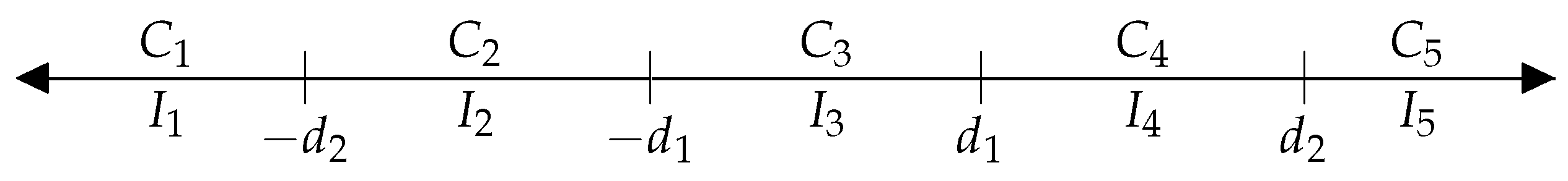
Let the objects to be evaluated be consecutively labeled as . In Thurstone-inspired paired comparison models, each object is assumed to be associated with a latent random variable , whose random value characterizes the object’s current performance. The expected value of the latent random variable associated with each object is denoted by . Decisions between two objects depend on the differences between the latent variables associated with them. We employ a five-option model, meaning that decisions can fall into one of five categories. In five-option models, the decisions are denoted by , , , , and , representing the opinions ’much worse’, ’slightly worse’, ’equal’, ’slightly better’, and ’much better,’ respectively. Each decision , for , corresponds to an interval . These intervals are mutually exclusive and cover the entire set . The boundaries of the intervals are determined by the parameters . Figure 1 illustrates these intervals and their associated decisions.
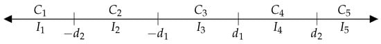
Figure 1.
The decision categories and their corresponding intervals in the five-option model: corresponds to ‘much worse’, to ‘slightly worse’, to ‘equal’, to ‘slightly better’, and to ‘much better’.
2.1. The Advantage-Insensitive Model
First, consider the basic five-option model with maximum likelihood parameter estimation. Now,
We suppose that are independent and identically distributed random variables. The probabilities can be expressed using the cumulative distribution function of , denoted by F. The probability of decision between the objects i and j—that is, when the difference is in the interval , for —is [37]:
Thurstone [31] assumed a Gaussian distribution for the random variables , which implies a Gaussian distribution for the differences . In fact, it is sufficient to require that the distribution function of , F, satisfies more general conditions: namely, , and it is continuously differentiable three times over; has a strictly log-concave probability density function; and is symmetric around zero [35]. Therefore, the logistic distribution can also be applied.
The data—that is, the results of the comparisons—are represented by the matrix . The superscript (0) indicates that the decisions were made without taking into account that one of the entities had an advantageous position compared to the other due to a certain factor. The value (where , ) denotes the number of cases in which object i was compared to object j and decision was made. Naturally, , , . Since only distinct objects are compared, , , . Due to the symmetry, , , .
The likelihood function given in Equation (7) expresses the probability of observing the elements in the data matrix given the parameters and . Using Equations (2)–(6), it can be written in the following form:
Its logarithm is
We can see that Equations (2)–(6) depend only on the differences between the expectations; consequently, the same holds for (7) and (8). Therefore, if one expectation is fixed, then (7) and (8) remain unchanged. To estimate the parameters, we seek the maximum value of this function. The maximum likelihood estimate of the parameter set ) is the argument at which the likelihood function (7) or, equivalently, the log-likelihood function (8) attains its maximum under the constraints and . Formally,
We note that in some cases, the constraint is replaced by the constraint .
2.2. The Advantage-Sensitive Model
There are cases in which one of the entities holds a distinguished position during the comparisons, while the other does not. We refer to this as the advantageous position and the other as the disadvantageous position. Think, for instance, of the advantage of making the first move in chess or the home-field advantage in certain sports. In such cases, it is worthwhile to incorporate this situational advantage into the model. We refer to these as advantage-sensitive models. The basic models that do not account for such advantages will be referred to as advantage-insensitive models. Now, we describe advantage-sensitive models. We suppose that during a comparison, one object is either in an advantageous or a disadvantageous position. The advantageous position increases the performance, while the disadvantageous position decreases it. Without loss of generality, we may assume that the measures of the increment and the decrease are equal. We introduce an advantage-effect parameter, denoted by b, to measure this. This parameter quantifies the average performance change caused by an advantageous or disadvantageous position. If the object is in an advantageous position, we add this parameter to its expectation since we believe that its strength increases in such a position. Conversely, if the object is in a disadvantageous position, we subtract it from , as we believe that its strength decreases in this case. In other words, this quantity adjusts the expected strengths of individual objects during the comparison, either increasing or decreasing them. Nevertheless, no assumption is made about the sign of the parameter.
Accordingly, if object i is in an advantageous position and j is in a disadvantageous one, then the difference between their performance is
In the reverse situation,
The superscripts (a) and (d) indicate the advantageous and disadvantageous positions, respectively. We do not restrict the value of b to positive numbers. If , the advantageous position generally results in a performance increase; if , it tends to reduce the performance. If , the position is essentially neutral and does not affect the performance.
The probabilities of the decisions are as follows, where the position of object i is indicated by the superscript [37].
It is clear that . As we distinguish the comparison results according to the positions, we now have two comparison matrices. The matrix contains the comparison data where object i is in the advantageous position, while matrix includes the number of comparisons where object i is in a disadvantageous position. These matrices satisfy the equalities for , and . The log-likelihood function is as follows:
In this model, the maximum likelihood estimate of the parameter set () is obtained by
2.3. Temporal Weighting
Experience shows that it is worthwhile to consider how much time has passed since the data were generated—that is, to adjust the data using temporal weighting [30]. This is especially important in cases where the strengths of individual objects change over time.
In such cases, we apply the following temporal weighting scheme: the result of the most recent comparison is taken with full weight (i.e., weight 1), while the weights of earlier comparison results are multiplied by a factor q at each time unit, where . For example, if the comparison result between objects i and j was generated 100 time units ago, then in the log-likelihood function (8), the multiplier is replaced by . The difference of 100 time units is referred to as the temporal distance. This procedure ensures that the influence of earlier comparison results decreases—and gradually diminishes—over time. This modification concerns only data matrices which provide the coefficients in the log-likelihood function. As the multiplier can even be a non-negative real number, optimization can be carried out, so estimation can be performed.
Let us define the elements of the weighted comparison matrices (w) as follows:
where t represents the temporal distance, measured in time steps, from the most recent comparison, and represent the comparison data obtained t time units earlier.
This time-weighting procedure will be applied to both data matrices and . If time weighting is applied, then the data matrices used for the evaluation are defined as
where M is the number of time steps to the current date. These data matrices will be included in the log-likelihood function (22) and will be used to compute the estimated strengths using (23).
2.4. The Model Specifications
In [38], Bradley and Terry defined a two-option model and assumed that the random variables followed a logistic distribution; that is,
This model is known in the literature as the Bradley–Terry model. We adopt a modification that retains the assumption of a logistic distribution—due to its computational efficiency—but extends the number of options from two to five. In honor of Bradley and Terry, we refer to this extension as the five-option Bradley–Terry model. We consider three variants of this model: we note the meaning of these abbreviations:
- The five-option advantage-insensitive model, abbreviated as ;
- The five-option advantage-sensitive model, abbreviated as ;
- The five-option advantage-sensitive model with temporal weighting, abbreviated as .
We also note the meaning of these abbreviations:
- refers to the use of the logistic cumulative distribution function, following Bradley and Terry;
- 5 indicates the number of options;
- P refers to the presence of a preferred (or an unpreferred) position;
- T signifies temporal weighting.
It is easy to see that the most general model is , with the other models as special cases.
- Setting recovers (i.e., no time decay);
- Setting reduces to (i.e., no advantage effect).
The models and their corresponding parameter settings are shown in Table 1.

Table 1.
Model parameter settings: b measures the advantage/disadvantage effect and is estimated from the data; q accounts for the temporal distance and is predefined.
We note that, while the advantage-effect parameter b is estimated within the model, the time-weighting parameter q is fixed in advance.
3. Metrics of the Models’ Forecasting Capability
The aim of this research is to forecast the outcomes of future comparisons, specifically in sports matches. If the strengths of the objects are evaluated, the probabilities of the outcomes can be estimated using Formulas (2)–(6) or (12)–(21), based on the estimated parameter values , , , and , if applicable. Although the model is capable of predicting five possible outcomes, we restrict ourselves to three: worse (loss), equal (draw), and better (win). There are two main reasons for this choice. First, these three outcomes are of primary interest. Second, they are commonly examined in the literature, allowing for a comparison of the model performance.
The predicted outcome is always the most probable among the options ‘better’, ‘equal’, and ‘worse’. The probability of ‘better’ will be computed as the sum of the probabilities of the options ‘much better’ and ‘slightly better’. Similarly, the probability of the option ‘worse’ is the sum of the probabilities ‘much worse’ and ‘slightly worse’.
Finding appropriate metrics is crucial for effectively comparing different models [39]. We now present the most commonly used metrics in the literature [24,29,32,39] for assessing the forecasting performance of models. Specifically, we consider four well-known metrics for evaluating predictive accuracy.
Fix an object and a comparison involving it. Let the outcome of the comparison be represented by a three-dimensional vector in the following formulas. The first coordinate corresponds to the outcome ‘worse’ from the perspective of the fixed object, the second to ‘equal’, and the third to ‘better’. When the result of a comparison is determined, the coordinate corresponding to the outcome takes the value 1, while the other coordinates are set to 0. represents the probability of the s-th outcome at a fixed comparison as predicted by the model. We recall the following metrics:
- LogLoss: The logarithmic loss metric quantifies the degree to which the model’s predictions deviate from the actual outcome in a logarithmic sense.This metric takes only positive values. The larger the predicted probability of the actual outcome, the smaller the LogLoss value. When the model assigns a higher probability to the true outcome, the LogLoss decreases, indicating less error. Consequently, a smaller average LogLoss corresponds to a better-performing model.
- The ranked probability score (RPS) is a metric used to assess the accuracy of multi-class predictions. It accounts for the “distance” between the predicted and actual outcomes by cumulatively measuring the deviation between the forecast probabilities and the true result. Therefore, if the predicted event is further from the actual outcome, the error will be larger. For example, if the actual result were ‘worse’ but we predicted ‘better’, the RPS would be higher than if we had predicted ‘equal’. Its values range between zero and one. For the RPS, smaller values indicate a better predictive performance.
- The Brier score (BS): The Brier score indicates the accuracy of individual predictions by measuring how far the predicted probabilities are from the actual outcomes.It takes only non-negative values, with its smallest value being 0 and its largest value equal to 2/3. In this metric, smaller values indicate a better forecasting ability.
- Accuracy (ACC): With this metric, we measure how many outcomes we correctly predicted out of all cases. Since the predicted result corresponds to the most probable outcome, we check whether the indices of the largest components in and (for the given case) coincide.Here, the arg max function returns the index of the coordinate where the vector attains its maximum value. If the maximum is not unique within , we select the first index among the candidates. For each prediction, this metric equals 1 if the outcome is correctly predicted and 0 otherwise. Averaging over all predictions gives the proportion of correct predictions. This average ranges from 0 to 1, with larger values indicating a better forecasting performance. A value of 1 means that all predictions are correct.
Additionally, we aimed to examine the prediction performance related to the position of the advantage-sensitive model. Based on the real outcomes, we constructed confidence intervals for the probabilities of the options ‘better’ and ‘worse’ in the advantageous position, as well as for the probability of the ‘equal’ option. Since a ‘better’ outcome in an advantageous position corresponds to a ‘worse’ outcome in a disadvantageous position, and vice versa, we do not present these values in the tables. The confidence interval containing the probability parameter with a confidence level is
Here, N denotes the total number of experiments (comparisons), is the number of occurrences of the event E, and . The event E can represent the decisions ‘worse’, ‘better’ in an advantageous position, or ‘equal’. In the case of the decision ‘equal’, one of the two objects must be in an advantageous position. We used a confidence level of ; therefore, =1.96. Our goal was to check whether the probabilities estimated by the models fell within the corresponding confidence intervals.
4. A Comparison of the Predictive Performance of the Models in Top European Football Championships
4.1. The Data Collection and Model Parameters
We aim to compare the performance of our models both against each other and against previously well-performing forecasting models. In [5], the authors thoroughly analyzed and compared several promising prediction models for team-sport outcomes. Consequently, we compare our models, presented in Section 2, to the method identified as the best in that article [5]. This method is an iterative version of the one-parameter Poisson model, as used in the paper by Lasek and Gagolewski, denoted there as and referred to here as . It uses information about goal differences and computes the team strength iteratively, thereby accounting for time effects. It also incorporates the home-field advantage—factors that are included in our most complex model as well. considers the number of goals using a five-option model, which distinguishes between small and large wins based on goal differences. A one-goal win is considered a small victory, i.e., the winner is ‘slightly better’ than the loser. A win by two or more goals is classified as a large victory, corresponding to the option ‘much better’. Similarly, losses are categorized as small or large. If the outcome is a draw, then the result of the comparison is ‘equal’. Our model also incorporates the home-field advantage through the parameter b and applies temporal weighting using data multiplied by to determine the team strengths.
Following the approach of Lasek and Gagolewski, we analyzed the match results from teams in the top five European football leagues. The time period covered three seasons [40], and we focused on teams that played in the top division of their respective countries in each of these seasons. To ensure the relevance of our measurements, we used the most recent data, selecting the 2021/22, 2022/23, and 2023/24 seasons. The first two seasons were used to train the models, while the results from the last season were used to test the predictions, ensuring that the models only had access to data available at least one day before each forecast. This meant that we predicted only the results of the matches in the 2023/24 season. First, we forecasted the results of the first round based on the results of the previous seasons. Then, the second round followed: the predictions were based on the results of the previous seasons and the first round, and so on.
In , temporal weighting is applied on a daily basis. For instance, if a match was played 5 days before the forecast date, its corresponding data is multiplied by . If it was played 500 days earlier, the data is multiplied by . Since the number of days across the three seasons is approximately , we chose . This value ensured that even the earliest matches retained some influence during the evaluation. The comparisons (matches) are gradually down-weighted over time; for example, a match from 1000 days ago receives a weight of .
For each of our models, we predicted the outcome with the highest estimated probability. We then compared the models using the four metrics presented in Section 3, which were also employed by Lasek and Gagolewski. The data were downloaded from the website [40]. In total, the results of 3066 matches were used: 546 from the English league (14 teams played home and away against each other each round) and 630 matches (among 15 teams) from each of the other leagues. The names of the teams that played in the top division in all three seasons across the different championships are listed in Table 2. The number of matches played by these teams is shown in Table 3. The abbreviation N.T. refers to the number of teams and N.M. to the number of matches in the different seasons.
Table 2.
The teams that played in the first division in all three seasons across the different championships.
Table 3.
The numbers of teams and matches in each league which were used in the predictions.
The ratio of draws, small wins, and large wins for each league is shown in Figure 2. Approximately 70–80% of matches end with a win, split roughly equally between small and large wins. This suggests that a significant amount of information can be captured when distinguishing between one-goal wins and wins by more than one goal. The ability to utilize this information is a key feature of the five-option model.
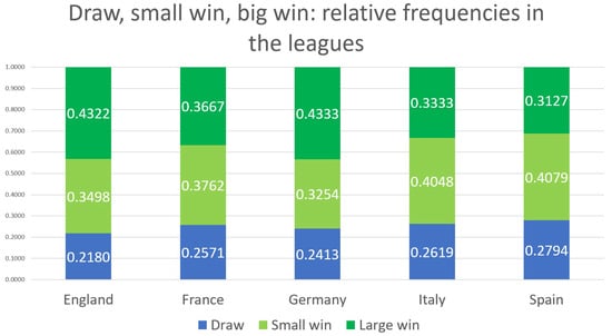
Figure 2.
The relative frequencies of draws, small wins, and large wins across the different leagues.
The number of predicted matches was 1022, and the numbers of correct predictions by , , , and were 527, 505, 534, and 535, respectively.
4.2. The Predictive Capabilities of the Investigated Models: Results and Discussion
The LogLoss values for the four methods (, , , and ) are shown in Table 4. The numerical values are around as low as those reported in the literature. It is clear that in terms of the average values, the model performs the worst, significantly trailing , followed by . The smallest average value is achieved by , indicating that it is the best-performing model overall, based on the average results shown in the last row. Relying on these average values is justified, as the model performance varies across leagues, and some models may predict specific outcomes better than others. For example, outperforms the other models for England, France, and Spain. In contrast, yields the best results for Germany and Italy. Nevertheless, on average, performs best across all leagues. When testing the LogLoss values of the model across countries, we find no significant differences between them: a one-way ANOVA testing the equality of means yields a p-value of 0.7703.
Table 4.
The LogLoss values, characterizing the predictions, defined by (28), computed for the different models in the case of the top five leagues and their averaged values.
The RPS metrics for each evaluation are shown in Table 5. They indicate that in some cases, the predictions deviate significantly from the actual outcomes. Overall, the RPS values can be considered moderately good.
Table 5.
The RPS values, characterizing the predictions, defined by (29), computed for the different models in the case of the top five leagues and their averaged values.
The ranking of the methods remains consistent in terms of the average results. For England, France, and Spain, outperforms both and ; nevertheless, the latter two achieve the best average performance overall. Meanwhile, the model—which does not incorporate the advantage—consistently ranks last.
Testing the equality of the expected RPS values for the model across countries, we do not find statistically significant differences among them (p-value = 0.4248).
The Brier score results are shown in Table 6. In this case, the ranking of the models shifts slightly based on the average metric. The model still performs the worst, significantly lagging behind the others. Next is , followed by , which marks a change in ranking compared to the previous two tables. continues to rank first overall.
Table 6.
The Brier score values, characterizing the predictions, defined by (30), computed for the different models in the case of the top five leagues and their averaged values.
Considering the predictive performance by country, in England, France, and Spain, both and outperform . However, in Germany and Italy, performs slightly better than and . It is worth noting that a Brier score around 0.2 is considered a good result for three-outcome models, such as those used in football match outcome predictions.
We also tested the equality of the expected Brier score values for the model across countries and found no significant differences among them (p-value = 0.7702).
Accuracy indicates the rate of correct outcome predictions. The results are presented in Table 7. An accuracy of 0.52 is already considered a competitive level of performance in the literature, especially when it is not the result of an overfitted machine learning model.
Table 7.
The accuracy values, characterizing the predicting ability, defined by (31), computed for the different models in the case of the top five leagues and their averaged values.
In this case, the ranking remains consistent with the Brier score: the model ranks last on average, while the model performs the best. The model ranks third, and comes in second, significantly outperforming . The improvement in the average accuracy for over , however, is not statistically significant.
Nevertheless, the results based on the accuracy metric differ from the others. While the rankings based on the LogLoss, RPSs, and Brier scores are largely consistent across countries, the accuracy-based rankings show notable differences.
What are particularly noticeable are the results from the Spanish league, where the model performs much better than the other three models, especially showing a significant advantage. In this league, some teams performed better at home (typically the top teams), while others earned more points away. On average, it can be said that the home-field advantage had a positive effect on the teams’ performance in the league. However, when similarly strong teams played, there were results that did not reflect the home-field advantage. This may explain why the model outperforms the others in this context.
We analyzed which teams’ match outcomes were the most and least predictable. The results can be found in Table 8. The leading teams tend to come from championships where one or two teams dominate. The worst ones are the medium-strength teams from the weaker leagues, especially among the Spanish teams. Moreover, they have a similar strength. This explains the lower average accuracy in the case of the Spanish league.
Table 8.
Upper and lower deciles of teams’ accuracy.
In summary, based on the four Table 4, Table 5, Table 6 and Table 7, the weakest-performing model was , which did not apply temporal weighting and did not account for the advantage associated with position. The and models performed similarly well according to the overall metrics, with having a slight edge over . The model that consistently performed best across all tables, when considering the average values, was the model, which applied temporal weighting alongside consideration of the possible positional advantage. We can conclude that both and are competitive with , the best predictive model reported in [5]. The model is not complex enough. It is advisable to use a more complex model for predictions, provided there is sufficient data to train it, as this generally leads to better results.
4.3. Model Fit: The Estimated Probabilities Computed by the Models and the Confidence Intervals Computed by Applying the Relative Frequencies
In this section, we demonstrate that models incorporating an advantage are suitable for detecting its presence. Specifically, this entails ensuring that the estimated probabilities calculated from the parameters fall within the corresponding confidence intervals. In football, an advantageous position corresponds to home-field matches. Since each season features only two matches between any two teams—one with an advantage and one without—we do not analyze the relative frequencies pairwise. Instead, we aggregate all of the wins and losses occurring in advantageous situations. Furthermore, since a win in an advantageous position mirrors a loss from the opposing team’s disadvantaged perspective, and vice versa, our analysis considers wins and losses in advantageous positions, as well as draws. Given that the model is advantage-insensitive (lacking the parameter b), this question does not apply in its case.
For each league, the estimated parameter values were positive—and, moreover, greater than 0.1—indicating that playing at home is indeed advantageous and generally favors the home team.
In the case of England, we calculated the relative frequencies of home wins, losses, and draws based on data for three years and used these to construct the confidence intervals. The relative frequencies, along with the lower and upper bounds of the confidence intervals, are shown in the first three columns of Table 9. We also computed the average probabilities derived from the estimated strengths in the and models; these are presented in columns 4 and 5 of Table 9.
Table 9.
The relative frequencies, confidence intervals computed based on them, and the average model-predicted probabilities for home wins, draws, and losses in the models and in the case of England.
Examining the data in Table 9, we observe that for the English championship, the estimated probabilities deviate only slightly from the midpoints of the intervals—that is, from the relative frequencies—in both the and models. In this case as well, the model demonstrates a slightly better performance than that of the model. These values are presented in columns 4 and 5 of Table 9.
For all five leagues, the relative frequencies, the endpoints of the confidence intervals, and the average probabilities predicted by the models are presented in Table 10. Here, the model performs slightly better than the model, although only marginally. Even in the worst case, the differences between the relative frequencies and the model-predicted probabilities do not exceed 0.0015.
Table 10.
The relative frequencies, confidence intervals computed based on them, and the average model-predicted probabilities for home wins, draws, and losses in the models and in the case of all top five leagues.
In summary, the probabilities predicted by the models closely approximate the relative frequencies of home wins, home losses, and draws. The models incorporate a parameter that represents the degree of advantage, determining both the direction and magnitude of the positional advantage on average. These models should also be applied in cases where it is unclear whether an advantage exists, as the variable b will take a value close to 0 if no such advantage is present.
For these models, the estimated parameter values for each championship are presented in Table 11. We also conducted likelihood ratio tests [41] to assess whether the parameter values differed significantly from zero. The test statistics and their corresponding significance levels are also reported in Table 11. As shown, the effect of the advantageous position is statistically significant in each country at all conventional significance levels.
Table 11.
The estimated values of the advantage-effect parameters, the calculated values of the test statistics, and the significance levels in the case of the and models.
4.4. The Best Four English Football Clubs’ Rankings in the 2023/24 Season
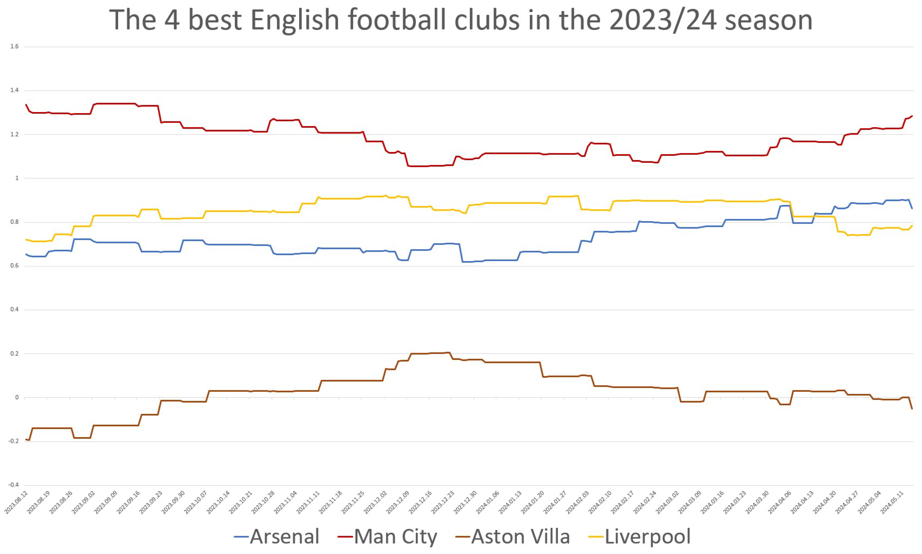
Since we tracked the teams’ strength on a daily basis, we were able to represent the changes in the teams’ strengths over time. In many previous publications, the English Premier League has been highlighted and praised as the best league [5,16]. Let us now examine the temporal changes in the strengths of the top teams in the English league. We selected the top four teams, as they qualified for the Champions League: Arsenal, Aston Villa, Liverpool, and Manchester City. The teams’ strengths were estimated under the constraint using the model. The official points and rankings of the teams are presented in Table 12, and the results of our evaluations are shown in Figure 3.
Table 12.
The best four English football clubs’ official points and rankings in the 2023/24 season.
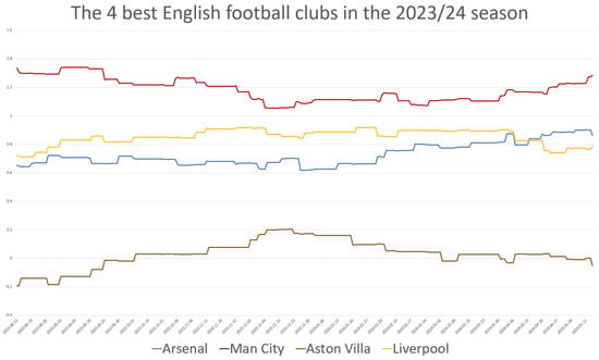
Figure 3.
The strengths of the top four English football clubs by week during the 2023/24 season.
Table 12 and Figure 3 clearly show that the final rankings in the two evaluations coincide. Manchester City is stronger than the other teams. The difference is small when considering the points but more significant when considering the estimated strengths. According to both evaluations, there is a large gap between the top three teams and the fourth, Aston Villa. Taking into account the results from earlier in the season has a balancing effect. Manchester City consistently ranks first, even though, based on points, the team only took the lead after the 33rd round—that is, near the end of the season. The model, which incorporates past information, predicted the final outcome more accurately than the points alone. Liverpool’s performance declined toward the end of the season, while Arsenal’s strength increased; these trends are clearly visible in Figure 3.
5. Summary
Three models were developed to evaluate sports performance and make predictions. These were compared with one another and with another high-performing model in terms of the predictive accuracy. The first innovative modification to the typical three-option Thurstone-motivated model was increasing the number of outcome categories from three to five, allowing for the consideration of the degree to which one team was better than the other. This extension makes it possible to incorporate additional information derived from the goal differences. Including more information can lead to a more accurate model.
A further modification involved incorporating the potential advantage associated with the position, which significantly improved the basic five-option model. The introduction of temporal weighting further refined the already high-performing model by accounting for time-dependent factors. To the best of the authors’ knowledge, these modifications have not previously been presented together in the literature. The resulting, most complex model—advantage-sensitive and incorporating temporal weighting—outperforms the simpler models and demonstrates an excellent predictive accuracy. On average, it performed better than all of the other models presented.
These models were compared to the best model from a recent, influential paper analyzing football match results. It is shown that the models developed in this paper are competitive with that model, as well as with the other prominent iterative models presented therein. Models that account for the potential advantage of playing at home are recommended for evaluating similar datasets. The positive effects of the home-field advantage have been quantified for the top five national leagues, and their significance has been statistically demonstrated. The confidence intervals constructed for the probabilities of home wins, home defeats, and draws—based on their relative frequencies—contain the probabilities estimated by the models, demonstrating a good fit.
In our models, the parameter characterizing the degree of the advantage effect is constant; that is, we assume it does not depend on the teams. However, in the case of the Spanish championship, we observed that this assumption was not supported by the match data: for some teams, the home-field position is not beneficial, while for others, it is. In the future, it would be worthwhile investigating whether team-specific advantage parameters could improve the predictive capability of the models.
This method can be applied not only to football but also to other sports where draws are possible and distinctions such as ‘small’ and ‘large victories’ are meaningful. Sports such as handball, ice hockey, and rugby fall into this category. In cases where draws do not occur—such as basketball or tennis—similar methods can still be applied by defining an advantage-sensitive, four-option model with temporal weighting. Beyond sports, this method can also be used in market research. For example, an advertising campaign may confer a competitive advantage, where temporal weighting reflects the timing of the campaign. If data are collected and evaluated using the model, the effect of the advertising campaign might be measurable.
Author Contributions
Conceptualization: C.M. and É.O.-M.; methodology: L.G.; software: L.G.; validation: L.G.; writing—original draft preparation: L.G.; writing—review and editing: É.O.-M. and C.M.; visualization: L.G.; supervision: C.M. All authors have read and agreed to the published version of the manuscript.
Funding
This work was implemented through the TKP2021-NVA-10 project with the support provided by the Ministry of Culture and Innovation of Hungary from the National Research, Development and Innovation Fund, financed under the 2021 Thematic Excellence Programme funding scheme.
Institutional Review Board Statement
Not applicable.
Informed Consent Statement
Not applicable.
Data Availability Statement
The football data were collected from https://www.football-data.co.uk/downloadm.php, accessed on 9 April 2025.
Conflicts of Interest
The authors declare no conflicts of interest.
Abbreviations
The following abbreviations are used in this manuscript:
| Iterative Poison model, one-variable version | |
| Five-option Bradley–Terry model | |
| Advantage-sensitive Bradley–Terry model with five options | |
| Advantage-sensitive Bradley–Terry model with five options and temporal weighting |
References
- Tay, F.E.; Shen, L. Economic and financial prediction using rough sets model. Eur. J. Oper. Res. 2002, 141, 641–659. [Google Scholar] [CrossRef]
- Foroni, C.; Marcellino, M.; Stevanovic, D. Forecasting the COVID-19 recession and recovery: Lessons from the financial crisis. Int. J. Forecast. 2022, 38, 596–612. [Google Scholar] [CrossRef] [PubMed]
- Teixeira, R.; Cerveira, A.; Pires, E.J.S.; Baptista, J. Enhancing weather forecasting integrating LSTM and GA. Appl. Sci. 2024, 14, 5769. [Google Scholar] [CrossRef]
- Akilan, T.; Baalamurugan, K.M. Automated weather forecasting and field monitoring using GRU-CNN model along with IoT to support precision agriculture. Expert Syst. Appl. 2024, 249, 123468. [Google Scholar] [CrossRef]
- Lasek, J.; Gagolewski, M. Interpretable sports team rating models based on the gradient descent algorithm. Int. J. Forecast. 2021, 37, 1061–1071. [Google Scholar] [CrossRef]
- Den Hartigh, R.J.; Niessen, A.S.M.; Frencken, W.G.; Meijer, R.R. Selection procedures in sports: Improving predictions of athletes’ future performance. Eur. J. Sport Sci. 2018, 18, 1191–1198. [Google Scholar] [CrossRef]
- Bunker, R.P.; Thabtah, F. A machine learning framework for sport result prediction. Appl. Comput. Inform. 2019, 15, 27–33. [Google Scholar] [CrossRef]
- Wilkens, S. Sports prediction and betting models in the machine learning age: The case of tennis. J. Sports Anal. 2021, 7, 99–117. [Google Scholar] [CrossRef]
- Horvat, T.; Job, J. The use of machine learning in sport outcome prediction: A review. Wiley Interdiscip. Rev. Data Min. Knowl. Discov. 2020, 10, e1380. [Google Scholar] [CrossRef]
- McCabe, A.; Trevathan, J. Artificial intelligence in sports prediction. In Proceedings of the Fifth International Conference on Information Technology: New Generations (ITNG 2008), Las Vegas, NV, USA, 7–9 April 2008; pp. 1194–1197. [Google Scholar] [CrossRef]
- Beal, R.; Norman, T.J.; Ramchurn, S.D. Artificial intelligence for team sports: A survey. Knowl. Eng. Rev. 2019, 34, e28. [Google Scholar] [CrossRef]
- Xu, T.; Baghaei, S. Reshaping the future of sports with artificial intelligence: Challenges and opportunities in performance enhancement, fan engagement, and strategic decision-making. Eng. Appl. Artif. Intell. 2025, 142, 109912. [Google Scholar] [CrossRef]
- Holmes, B.; McHale, I.G. Forecasting football match results using a player rating based model. Int. J. Forecast. 2024, 40, 302–312. [Google Scholar] [CrossRef]
- Arntzen, H.; Hvattum, L.M. Predicting match outcomes in association football using team ratings and player ratings. Stat. Model. 2021, 21, 449–470. [Google Scholar] [CrossRef]
- Baker, R.D.; McHale, I.G. Forecasting exact scores in National Football League games. Int. J. Forecast. 2013, 29, 122–130. [Google Scholar] [CrossRef]
- Gyarmati, L.; Orbán-Mihálykó, É.; Mihálykó, C.; Vathy-Fogarassy, Á. Aggregated Rankings of Top Leagues’ Football Teams: Application and Comparison of Different Ranking Methods. Appl. Sci. 2023, 13, 4556. [Google Scholar] [CrossRef]
- Luiz, L.E.; Fialho, G.; Teixeira, J.P. Is Football Unpredictable? Predicting Matches Using Neural Networks. Forecasting 2024, 6, 1152–1168. [Google Scholar] [CrossRef]
- Groll, A.; Ley, C.; Schauberger, G.; van Eetvelde, H. A hybrid random forest to predict soccer matches in international tournaments. J. Quant. Anal. Sports 2019, 15, 271–287. [Google Scholar] [CrossRef]
- Stübinger, J.; Mangold, B.; Knoll, J. Machine learning in football betting: Prediction of match results based on player characteristics. Appl. Sci. 2019, 10, 46. [Google Scholar] [CrossRef]
- Constantinou, A.C.; Fenton, N.E.; Neil, M. pi-football: A Bayesian network model for forecasting association football match outcomes. Knowl.-Based Syst. 2012, 36, 322–339. [Google Scholar] [CrossRef]
- Markopoulou, C.; Papageorgiou, G.; Tjortjis, C. Diverse Machine Learning for Forecasting Goal-Scoring Likelihood in Elite Football Leagues. Mach. Learn. Knowl. Extr. 2024, 6, 1762–1781. [Google Scholar] [CrossRef]
- González-Díaz, J.; Hendrickx, R.; Lohmann, E. Paired comparisons analysis: An axiomatic approach to ranking methods. Soc. Choice Welf. 2014, 42, 139–169. [Google Scholar] [CrossRef]
- Mavi, R.K.; Mavi, N.K.; Kiani, L. Ranking football teams with AHP and TOPSIS methods. Int. J. Decis. Sci. Risk. Manag. 2012, 4, 108–126. [Google Scholar] [CrossRef]
- Hvattum, L.M.; Arntzen, H. Using ELO ratings for match result prediction in association football. Int. J. Forecast. 2010, 26, 460–470. [Google Scholar] [CrossRef]
- Koopman, S.J.; Lit, R. A dynamic bivariate Poisson model for analysing and forecasting match results in the English Premier League. J. R. Stat. Soc. 2015, 178, 167–186. [Google Scholar] [CrossRef]
- López-Barrientos, J.D.; Zayat-Niño, D.A.; Hernández-Prado, E.X.; Estudillo-Bravo, Y. On the Élö–Runyan–Poisson–Pearson Method to Forecast Football Matches. Mathematics 2022, 10, 4587. [Google Scholar] [CrossRef]
- Foulley, J.-L. A simple Bayesian procedure for forecasting the outcomes of the UEFA Champions League matches. J. Soc. Fr. Stat. 2015, 155, 38–50. [Google Scholar]
- Krzywanski, J.; Sosnowski, M.; Grabowska, K.; Zylka, A.; Lasek, L.; Kijo-Kleczkowska, A. Advanced Computational Methods for Modeling, Prediction and Optimization—A Review. Materials 2024, 17, 3521. [Google Scholar] [CrossRef]
- Koopman, S.J.; Lit, R. Forecasting football match results in national league competitions using score-driven time series models. Int. J. Forecast. 2019, 35, 797–809. [Google Scholar] [CrossRef]
- Held, L.; Vollnhals, R. Dynamic rating of European football teams. IMA J. Manag. Math. 2005, 16, 121–130. [Google Scholar] [CrossRef]
- Thurstone, L. A law of comparative judgment. Psychol. Rev. 1927, 34, 273–286. [Google Scholar] [CrossRef]
- Ley, C.; de Wiele, T.V.; Eetvelde, H.V. Ranking soccer teams on the basis of their current strength: A comparison of maximum likelihood approaches. Stat. Model. 2019, 19, 55–73. [Google Scholar] [CrossRef]
- Rao, P.V.; Kupper, L.L. Ties in paired-comparison experiments: A generalization of the Bradley-Terry model. J. Am. Stat. Assoc. 1967, 62, 194–204. [Google Scholar] [CrossRef]
- Glenn, W.A.; David, H.A. Ties in paired-comparison experiments using a modified Thurstone-Mosteller model. Biometrics 1960, 16, 86–109. [Google Scholar] [CrossRef]
- Orbán-Mihálykó, É.; Mihálykó, C.; Koltay, L. Incomplete paired comparisons in case of multiple choice and general log-concave probability density functions. Cent. Eur. J. Oper. Res. 2019, 27, 515–532. [Google Scholar] [CrossRef]
- Gyarmati, L.; Mihálykó, C.; Orbán-Mihálykó, É. Algorithm for Option Number Selection in Stochastic Paired Comparison Models. Algorithms 2024, 17, 410. [Google Scholar] [CrossRef]
- Walpole, R.E.; Myers, R.H.; Myers, S.L.; Ye, K. Probability and Statistics for Engineers and Scientists; Macmillan: New York, NY, USA, 1993; p. 53. [Google Scholar]
- Bradley, R.A.; Terry, M.E. Rank analysis of incomplete block designs: I. The method of paired comparisons. Biometrika 1952, 39, 324–345. [Google Scholar] [CrossRef]
- Constantinou, A.C.; Fenton, N.E. Solving the Problem of Inadequate Scoring Rules for Assessing Probabilistic Football Forecast Models. J. Quant. Anal. Sports 2012, 8, 1–14. [Google Scholar] [CrossRef]
- European Football Results and Betting Odds. Available online: https://www.football-data.co.uk/downloadm.php (accessed on 5 May 2025).
- Wilks, S.S. The Large-Sample Distribution of the Likelihood Ratio for Testing Composite Hypotheses. Ann. Math. Stat. 1938, 9, 60–62. [Google Scholar] [CrossRef]

Disclaimer/Publisher’s Note: The statements, opinions and data contained in all publications are solely those of the individual author(s) and contributor(s) and not of MDPI and/or the editor(s). MDPI and/or the editor(s) disclaim responsibility for any injury to people or property resulting from any ideas, methods, instructions or products referred to in the content. |
© 2025 by the authors. Licensee MDPI, Basel, Switzerland. This article is an open access article distributed under the terms and conditions of the Creative Commons Attribution (CC BY) license (https://creativecommons.org/licenses/by/4.0/).