Abstract
We examine how prior specification affects the Bayesian Dirichlet Auto-Regressive Moving Average (B-DARMA) model for compositional time series. Through three simulation scenarios—correct specification, overfitting, and underfitting—we compare five priors: informative, horseshoe, Laplace, mixture of normals, and hierarchical. Under correct model specification, all priors perform similarly, although the horseshoe and hierarchical priors produce slightly lower bias. When the model overfits, strong shrinkage—particularly from the horseshoe prior—proves advantageous. However, none of the priors can compensate for model misspecification if key VAR/VMA terms are omitted. We apply B-DARMA to daily S&P 500 sector trading data, using a large-lag model to demonstrate overparameterization risks. Shrinkage priors effectively mitigate spurious complexity, whereas weakly informative priors inflate errors in volatile sectors. These findings highlight the critical role of carefully selecting priors and managing model complexity in compositional time-series analysis, particularly in high-dimensional settings.
1. Introduction
Compositional time series, in which observations are vectors of proportions constrained to sum to one, arise in a wide range of applications. For instance, market researchers track evolving shares of competing products [1] ecologists monitor species composition over time, and sociologists or political scientists follow shifting demographic or budgetary profiles [2]. In each case, the data lie within a simplex, making the Dirichlet model a common starting point [3,4]. However, when temporal dependence is also present—for example, today’s composition influences tomorrow’s—the Dirichlet framework must be extended to account for dynamics in a way that respects the simplex constraints.
Several approaches have emerged to handle dynamic compositional data, notably by coupling the Dirichlet with Auto-Regressive Moving Average (ARMA)-like structures [5], by using a logistic-normal representation [6], or by adopting new families of innovation distributions [7]. Others have adapted the model to cope with zeros [8] or extreme heavy-tailed behaviors. In particular, the Bayesian Dirichlet Auto-Regressive Moving Average (B-DARMA) model [9] addresses key compositional modeling challenges by introducing Vector Auto-Regression (VAR) and Vector Moving Average (VMA) terms for multivariate compositional data. Under B-DARMA, each day’s, or time point’s, composition is Dirichlet-distributed with parameters that evolve with a VARMA process in the additive log-ratio space, capturing both compositional constraints and serial correlation.
Although B-DARMA provides a flexible foundation, practitioners must still specify priors for potentially high-dimensional parameter spaces, which can be prone to overfitting or omitted-lag bias. The growing literature on Bayesian shrinkage priors offers numerous solutions, from global–local shrinkage frameworks [10] to hierarchical approaches [11], along with classic spike-and-slab [12,13] and Laplace priors [14]. These priors can encourage sparsity and suppress extraneous lags in over-parameterized models, a crucial feature for many real-world compositional applications in which the number of possible lags or covariates exceeds the sample size. The horseshoe prior [15,16] has shown particular promise in forecasting studies where only a minority of parameters matter and many are effectively zero. At the same time, hierarchical shrinkage [11] facilitates partial pooling across related coefficient blocks, an appealing property when working with multi-sector or multi-species compositions.
In this paper, we systematically investigate how five different prior families—informative normal, horseshoe, Laplace, spike-and-slab, and hierarchical shrinkage—affect parameter recovery and predictive accuracy in the B-DARMA model. We compare their performance across three main scenarios using simulated data: (i) correct specification, where the model order matches the true process; (ii) overfitting, where extraneous VAR/VMA terms inflate model dimensionality; and (iii) underfitting, where key VAR/VMA terms are missing altogether. Our findings confirm that shrinkage priors—especially horseshoe and hierarchical variants—can successfully rein in overfitting, providing more robust parameter estimates and improved forecasts. Conversely, no amount of shrinkage compensates for omitted terms, highlighting the need for careful model specification.
To demonstrate the practical impact, we also apply B-DARMA to daily S&P 500 sector trading data, a large-scale compositional time series characterized by multiple seasonalities and long-lag behavior. Consistent with the simulation insights, we find that more aggressive shrinkage priors significantly reduce spurious complexity and improve forecast accuracy, especially for volatile sectors. These outcomes reinforce that while B-DARMA provides a natural scaffolding for compositional dependence, judicious prior selection and meaningful lag choices are pivotal.
In the remainder of this paper, we first review the B-DARMA model (Section 2) and outline how our five prior families (informative, horseshoe, Laplace, spike-and-slab, and hierarchical) encode distinct shrinkage behaviors. We then present the design and results of three simulation studies (Section 3 and Section 4) before turning to the empirical S&P 500 application (Section 5). We conclude with recommendations for practitioners modeling compositional time series with complex temporal dynamics and large parameter counts.
2. Background
2.1. Compositional Data and the Dirichlet Distribution
Compositional data consist of vectors of proportions, each strictly between zero and one and summing to unity [3]. Formally, let
where each and The vector resides in the -dimensional simplex.
A natural choice for modeling such compositional vectors is the Dirichlet distribution. In its basic form, a Dirichlet random vector is parameterized by a concentration vector with . The probability density function is
where
and is the Gamma function. This parameterization captures both the support of compositional data (the simplex) and the potential correlation structure among components.
2.2. B-DARMA Model
To capture temporal dependence in compositional data, the Bayesian Dirichlet Auto-Regressive Moving Average (B-DARMA) model [9] augments the Dirichlet framework with VAR and VMA dynamics. Specifically, for each time , let be the observed composition. We assume
with density , where ’ is the mean composition and is a precision parameter. Both and may vary with time.
- ALR link.
Because each lies in the simplex, we map it to an unconstrained -dimensional vector via the additive log-ratio transform
We denote
- VARMA structure.
To incorporate serial dependence, we assume that follows a vector VARMA process in the transformed space
for , where . In this notation, and are each coefficient matrices; is a known covariate matrix, including any intercepts, trends, or seasonality; and is a vector of regression coefficients shared across the components.
- Precision parameter.
The Dirichlet precision can also evolve over time. For an -vector of covariates , we set
with . In the absence of covariates, we simply have for all t, so becomes a constant.
- Parameter vector.
We gather all unknown parameters into a vector of length C,
where , , and , and is the j-th element of . The total number of free parameters is thus
Bayesian inference begins by positing a prior distribution over the model parameters . Bayes’ theorem updates this prior to form the posterior
where
and is the normalizing constant obtained by integrating over . Each follows the Dirichlet likelihood (1).
Next, to generate predictions for the subsequent S time points, , we construct the joint predictive distribution
In practice, analysts often summarize this distribution at future time points by reporting measures such as the posterior mean or median.
2.3. Bayesian Shrinkage Priors for B-DARMA Coefficients
In a fully Bayesian approach, all unknown parameters in the B-DARMA model—including the VARMA coefficients in and , the regression vector , and the precision-related parameters —require prior distributions. Different shrinkage priors can produce significantly different outcomes, particularly in high-dimensional or sparse settings where many coefficients may be small. This section discusses five popular priors (normal, horseshoe, Laplace, spike-and-slab, and hierarchical), highlighting how each encodes shrinkage or sparsity assumptions.
An informative normal prior serves as a straightforward baseline. We model each coefficient by . The mean a often defaults to zero unless prior knowledge indicates a different center. The variance determines the shrinkage strength; smaller yields tighter concentration around a. In B-DARMA applications, it may be sensible to set for the VARMA parameters if they are believed to be small on average, whereas for covariates , a smaller prior variance such as can reflect stronger beliefs that regression effects are modest.
The horseshoe prior [15] is well-suited for sparse problems. We model each coefficient as , with a global scale and local scales . Large local scales allow some coefficients to remain sizable, whereas most are heavily shrunk. This can be beneficial if the B-DARMA model includes many possible lags or covariates, only a small subset of which are expected to matter for compositional forecasting.
A Laplace (double-exponential) prior [14] employs the density . This enforces an -type penalty that can drive many coefficients close to zero while still allowing moderate signals to persist. The scale b can be chosen a priori or assigned its own hyperprior, such as a half-Cauchy, so that the data adaptively determine the shrinkage level. In a B-DARMA context, choosing a smaller b for high-dimensional VARMA terms can prevent spurious estimates from inflating the parameter space.
A spike-and-slab prior [12] can introduce explicit sparsity by placing a point mass at zero. Let be the mixing parameter for the jth coefficient. Then, each coefficient follows the mixture
where is the Dirac measure at zero. Coefficients drawn from the spike component remain exactly zero, effectively excluding them from the model, while coefficients from the slab remain freely estimated. This setup allows the B-DARMA specification to adapt by discarding irrelevant lags or covariates.
A hierarchical shrinkage prior [17] can encourage partial pooling across groups of coefficients. We model each coefficient by and then place a half-Cauchy prior on . In B-DARMA, one could assign separate group scales to the AR, MA, and regression blocks, thereby allowing the model to learn an appropriate overall variability for each group of parameters.
These priors differ in how strongly they push coefficients toward zero and whether they favor a few large coefficients or moderate shrinkage for all. The normal prior provides a baseline continuous shrinkage, the horseshoe prior excels when only a minority of parameters are truly large, the Laplace prior induces an -type penalty that can zero out many coefficients, the spike-and-slab prior explicitly discards some parameters, and the hierarchical prior alternative enables group-level learning of shrinkage scales. The next sections illustrate how these choices affect both parameter recovery and compositional forecasting in various simulation and real-data scenarios.
2.4. Posterior Computation
All B-DARMA models are fit with STAN [18] in R using Hamiltonian Monte Carlo. We run 4 chains, each with 500 warm-up and 750 sampling iterations, yielding posterior draws. The sampler uses adapt_delta = 0.85, max_treedepth = 11, and random initial values drawn uniformly from [−0.25, 0.25].
2.5. Stationarity and Structural Considerations
- Open theoretical gap. B-DARMA inherits the difficulty noted by Zheng and Chen [5]: after the additive-log-ratio (ALR) link, the innovation is not a martingale-difference sequence (MDS). Consequently, classical stationarity results for VARMA (p,q) processes do not transfer directly, and a full set of strict- or weak-stationarity conditions remains an open problem ([9] [IJF, §2.2]).
- Why Bayesian inference remains valid. Bayesian estimation proceeds via the joint posterior , which does not require the likelihood-error sequence to be an MDS [19]. We therefore regard B–DARMA as a flexible likelihood-based filter for compositional time series rather than assume that the fitted parameters represent a strictly stationary data-generating process.
3. Simulation Studies
We conduct three simulation studies to investigate how different priors affect parameter inference and forecasting in a B-DARMA model. All studies use the same sparse DARMA(2,1) data-generating process (DGP) but vary the fitted model to be correctly specified, deliberately overfitted, or underfitted. We first describe the DGP and the priors considered, and then outline the study designs and performance metrics.
3.1. Data-Generating Process
We simulate a six-dimensional compositional time series , each component constrained to sum to one. The true process is DARMA(2,1) with fixed precision , , and , a identity matrix. We set our VAR and VMA matrices to
We initialize and from , simulate observations, and replicate this procedure 50 times. We focus on posterior inference for and , as well as forecasting accuracy.
3.2. Prior Distributions and Hyperparameters
We specify five candidate priors for the coefficient vectors: normal (mean 0, variance 1), horseshoe (global and local scales), Laplace (scale ), spike-and-slab (with local mixing parameters ), and hierarchical normal (with a half-Cauchy prior on the group-level scale). Although these priors remain the same across simulations, they are applied to different sets of coefficients: and in Simulation 1; –– and in Simulation 2; and and in Simulation 3. For the Dirichlet precision parameter, we use . The normal prior on is , and the Laplace and hierarchical normal versions adopt smaller scales to impose stronger shrinkage on intercepts.
3.3. Study Designs
We fit three B-DARMA specifications to the same DARMA(2,1) data:
- Study 1 (Correct Specification): B-DARMA(2,1) matches the true DGP.
- Study 2 (Overfitting): B-DARMA(4,2) includes extraneous higher-order VAR and VMA terms.
- Study 3 (Underfitting): B-DARMA(1,0) omits the second VAR lag and the MA(1) term.
Each configuration is paired with each of the five priors, yielding 15 total fitted models. We repeat the simulation for 50 synthetic datasets of length T.
3.4. Evaluation Metrics
We assess both parameter recovery and forecasting performance. Let be a true parameter and be the posterior mean from simulation s. We compute
along with 95% credible-interval coverage and interval length. If a parameter is omitted (as in underfitting), we exclude it from these summaries.
For forecasting, we use the first 80 points for training and the remaining 20 points for testing. Let be the posterior mean forecast at time t in simulation s. We define
where denotes the true composition in the test set for the s-th simulation. Each of the three study designs is then evaluated under each of the five priors, illuminating how prior choice interacts with model misspecification.
4. Results
The summarized parameter estimation results of the three simulation studies are shown in Table 1, Table 2, Table 3, Table 4 and Table 5, and the summarized forecast results are shown in Table 2, Table 3, Table 4, Table 5 and Table 6.

Table 1.
Parameter estimation summary for simulation study 1 (correct specification). We show the mean bias, RMSE, average credible-interval length, and coverage for each prior, summarizing over all parameters in each of and . Lower RMSE and shorter intervals typically indicate more effective shrinkage, while coverage near the nominal 0.95 is desirable.
Table 2.
Forecast performance summary across simulations. M-RMSE is the mean (across simulations) of the root mean squared error on the test set, and SD-RMSE is its standard deviation.
Table 3.
Parameter estimation summary for simulation study 2 (overfitting). This table reflects the setting where the fitted model (B-DARMA(4,2)) exceeds the true DARMA(2,1) order. We report the mean bias, RMSE, credible-interval length, and coverage for each prior and parameter.
Table 4.
Forecasting performance ratios for mean RMSE and SD RMSE. “S2” = overfitting scenario; “S3” = underfitting scenario; “S1” = correct DGP. Columns show how each simulation compares in terms of the mean RMSE (left) and SD RMSE (right). Ratios indicate worse performance relative to the denominator; indicates better.
Table 5.
Parameter estimation summary for simulation study 3 (underfitting). This table reports key metrics (mean bias, RMSE, average CI length, and coverage) when crucial AR(2) and MA(1) terms are omitted. All priors suffer from higher errors and coverage shortfalls, indicating that structural misspecification is the dominant source of inaccuracy.
Table 6.
Forecasting performance ratios within simulations (best model as denominator).
4.1. Study 1: Correct Model Specification (DARMA(2,1))
4.1.1. Parameter Estimation
Table 1 shows the results for the correctly specified DARMA(2,1). All priors yield estimates that align with the true parameter values, and both bias and RMSE remain modest. Certain shrinkage priors, including the horseshoe and Laplace, produce slightly lower RMSE and narrower intervals than the normal prior. Hierarchical priors also reduce parameter uncertainty to some extent, although the differences relative to other shrinkage methods are not pronounced. Under spike-and-slab, small but non-zero signals can be set to zero, occasionally lowering coverage (for example, a coverage rate of 0.8240 for the intercept ).
4.1.2. Forecasting Performance
In Table 2 (Sim. 1 columns), the average forecast RMSE spans 0.031–0.032, with minimal variation among priors. The horseshoe, Laplace, and hierarchical priors provide slight gains in predictive accuracy compared to the informative normal or spike-and-slab approaches.
4.2. Study 2: Overfitting Scenario (B-DARMA(4,2))
4.2.1. Parameter Estimation
When B-DARMA(4,2) is applied to data generated by a DARMA(2,1) process, additional VAR and VMA terms that should be zero are introduced. In Table 3, relatively large biases and inflated RMSE values appear under the informative normal prior for these extraneous coefficients. Horseshoe priors shrink many of those coefficients near zero, reflected in low RMSE (for instance, 0.0176 or 0.0161 for and ) and coverage rates close to the nominal level. Spike-and-slab also suppresses unwanted terms, although borderline signals may be excessively reduced.
4.2.2. Forecasting Performance
The forecast RMSE under the overfitting conditions is listed in Table 2 (Sim. 2 columns). Higher errors (0.0341) are observed for the informative normal prior, while the horseshoe prior produces the lowest RMSE (0.0315). The Laplace and hierarchical approaches also outperform the weakly regularized alternative. The ratios in Table 4 indicate that the horseshoe’s forecast RMSE in the overfitted model differs little from the correctly specified case.
4.3. Study 3: Underfitting Scenario (B-DARMA(1,0))
4.3.1. Parameter Estimation
In Table 5, broad increases in RMSE and reduced coverage are noted when the second VAR lag and the VMA(1) term are omitted, regardless of the prior used. Horseshoe, Laplace, and spike-and-slab cannot compensate for missing structural components, which leads to biased AR(1) estimates and coverage gaps. The hierarchical prior exhibits comparable issues.
4.3.2. Forecasting Performance
The forecast RMSE remains near 0.032–0.033, indicating a 3–4% rise over the correct specification. This shortfall is consistent across priors (Table 4), confirming that underspecification cannot be resolved by shrinkage.
4.4. Overview of Results
These simulations illustrate how model specification and prior choice jointly affect B-DARMA outcomes. Under a correctly specified DARMA(2,1), all priors capture the process well, although the horseshoe and hierarchical priors yield slightly lower RMSE and narrower intervals. In overfitted scenarios, shrinkage priors—especially the horseshoe—readily suppress spurious parameters and maintain robust forecasts. Underfitting cannot be mitigated by any prior, as the exclusion of critical VAR or VMA terms inflates bias and diminishes coverage. Further exploration of alternative coefficient matrices, described in the Supplementary Materials, reinforces these findings: shrinkage priors protect against overfitting but cannot repair underspecified models. The horseshoe, Laplace, and hierarchical priors yield stable forecasts across various parameter settings, whereas the informative normal approach is more susceptible to inflated estimates in large or sparse models.
5. Application to S&P 500 Sector Trading Values
5.1. Motivation and Data Description
A fixed daily trading value in the S&P 500 is allocated across different sectors, giving rise to compositional data that captures how investors distribute their capital each day. Tracking these proportions over time can reveal macroeconomic trends, sector rotation, and shifts in investor sentiment. In our analysis, we examined the daily proportions of eleven S&P 500 sectors from January 2021 to December 2023. These sectors include the following:
- Technology: software, hardware, and related services.
- Healthcare: pharmaceuticals, biotechnology, and healthcare services.
- Financial Services: banking, insurance, and investment services.
- Consumer Discretionary: non-essential goods and services.
- Industrials: manufacturing, aerospace, defense, and machinery.
- Consumer Staples: essential goods, such as food and household items.
- Energy: oil, gas, and renewable resources.
- Utilities: public services such as electricity and water.
- Real Estate: REITs and property management.
- Materials: chemicals, metals, and construction materials.
- Communication Services: media, telecommunication, and internet services.
Let denote the dollar trading value executed in sector k on trading day t for ( sectors). The market-wide total is
and the composition we analyze is the vector of sector shares
The stationarity (or non-stationarity) of the compositional time series is independent of that of the gross total : may drift without affecting the stationarity of the shares, and, conversely, the shares could be non-stationary even if is itself stationary.
We used data from 1 January 2021 to 30 June 2023, for training, as shown in Figure 1. The forecast evaluation was conducted on 126 trading days, spanning 1 July through 31 December 2023.
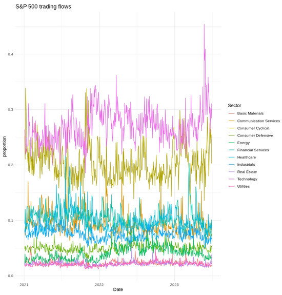
Figure 1.
Daily proportions of S&P 500 trading flows by sector from January 2021 to June 2023. Sector colors are indicated in the legend.
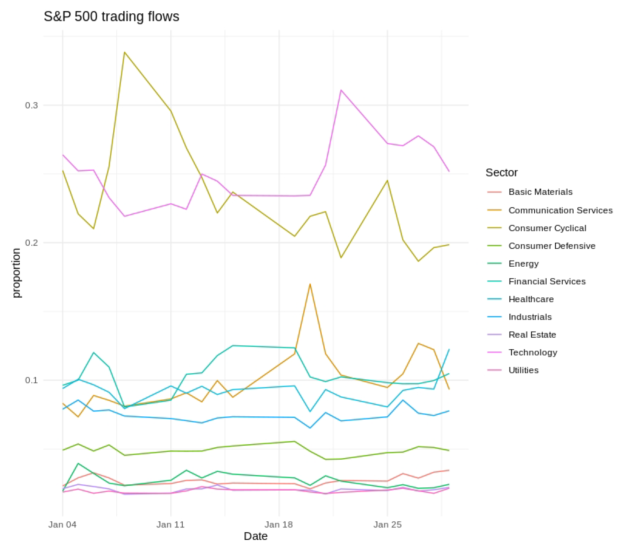
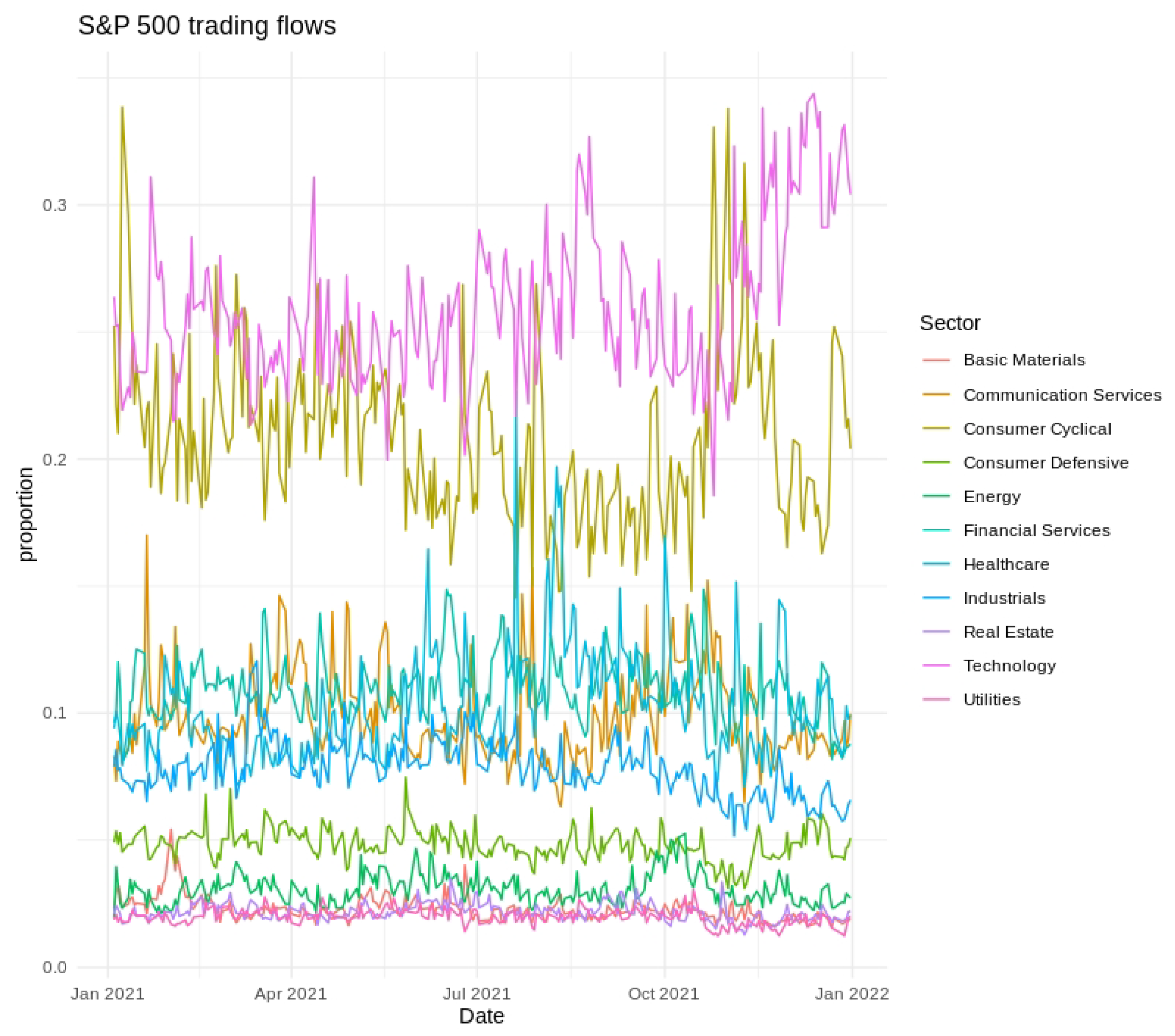
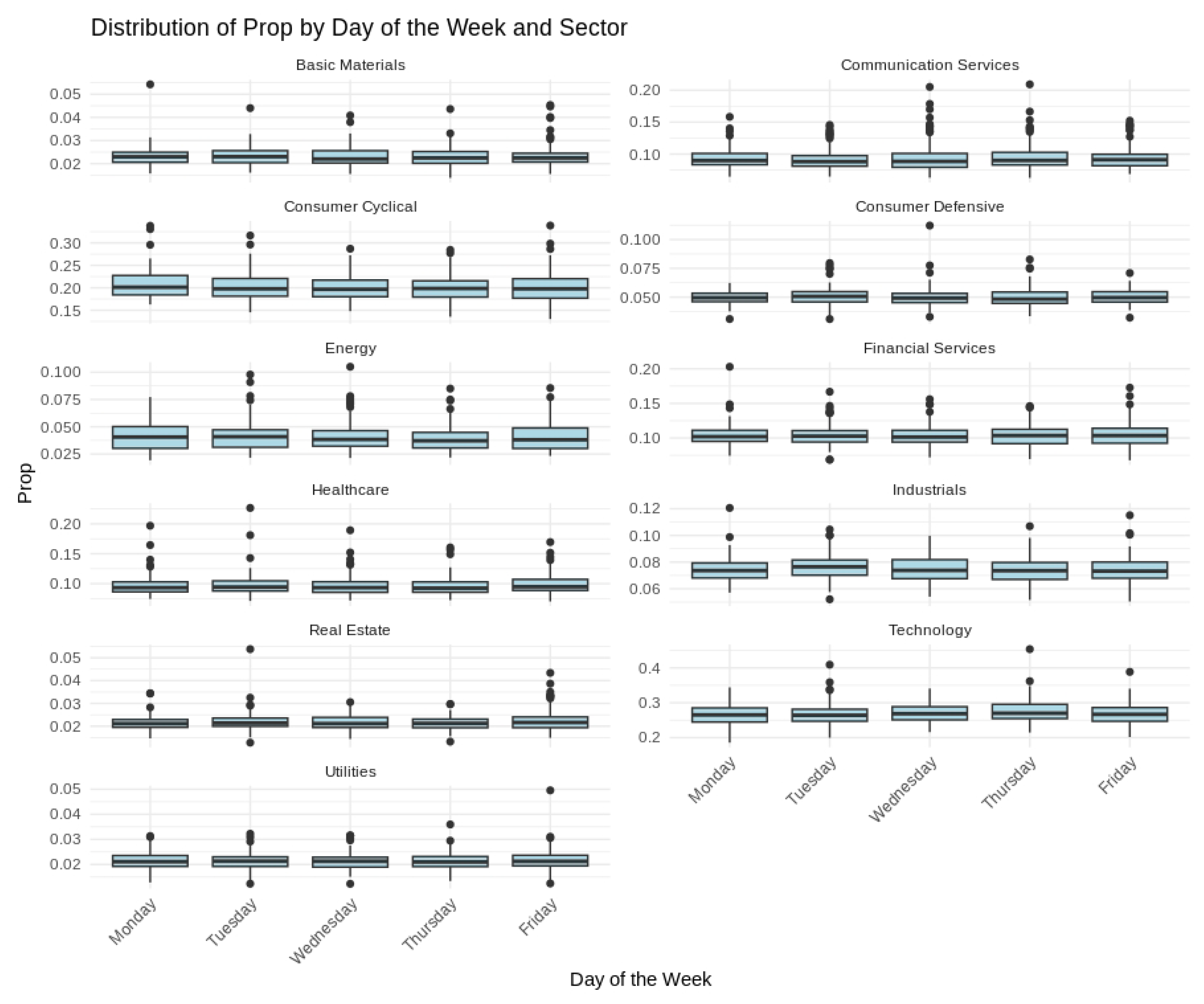
Short-term variability, cyclical tendencies, and gradual long-term shifts emerged across the series. Technology and Financial Services consistently held the largest fractions of the fixed daily trading value, whereas Utilities and Real Estate occupied much smaller shares. Day-to-day fluctuations tended to be more pronounced in Consumer Discretionary and Communication Services, indicating greater sensitivity to rapidly changing market conditions. Seasonal patterns and moderate differences across weekdays were also evident, as illustrated in Figure 2, Figure 3 and Figure 4, further underscoring the multifaceted nature of sector-level trading dynamics.
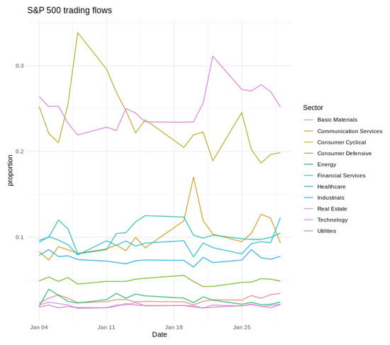
Figure 2.
Daily S&P 500 trading flows by sector for January 2021. Sector colors are indicated in the legend.

Figure 3.
Time series of S&P 500 trading flows from January 2021 to January 2022. Sector colors are indicated in the legend.
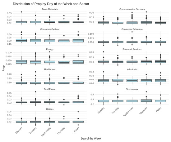
Figure 4.
Box plots of S&P 500 sector trading proportions by day of the week.
Model specification (purposeful over-parameterization). A model is fitted by design with a lag order that exceeds the horizon over which sector reallocations are generally thought to propagate. Ten trading days (≈ two calendar weeks), therefore, represent a deliberate overfit, allowing us to evaluate how strongly the global–local shrinkage priors suppress redundant dynamics. Each sector’s additive-log-ratio is regressed on its own composition at lags , yielding VAR coefficients in the matrices .
Seasonality is modeled with Fourier bases that are fixed regardless of the chosen lag: two sine–cosine pairs capture the 5-day trading cycle (Monday–Friday), and five pairs capture the annual cycle of roughly 252 trading days. These 14 terms, together with a sector-specific intercept, form the design matrix for the linear predictor; the same seasonal structure enters the model for the Dirichlet precision .
In total, the specification estimates 1165 parameters: 1000 VAR coefficients, 140 seasonal coefficients, 10 intercepts, and 15 precision-related terms. The intentionally generous lag order thus functions as a stress test.
5.2. Priors and Hyperparameters
For all priors, the intercept in is given an prior, and all seasonal Fourier terms in receive .
Under the informative normal prior, every element of is modeled with an prior, and each element of has an prior.
The Laplace prior [14] is implemented via an exponential mixture: each coefficient satisfies with , leading to an overall Laplace prior. We set and for and , respectively.
For the spike-and-slab prior [12], each coefficient is drawn from a mixture: with probability or with probability , where is the mixing weight.
The horseshoe prior [15] introduces one global scale parameter and local scales , all drawn from . Each coefficient then follows .
Finally, under the hierarchical prior [17], the coefficients are partitioned into three groups: (i) the elements of , (ii) the diagonal entries of each lag matrix , and (iii) the off-diagonal entries of each . Then, the coefficients in are modeled as , while for each lag p in , the diagonal entries follow and the off-diagonal entries follow .
5.3. Evaluation Metrics and Forecasting
A B-DARMA(10,0) model was fit with each of the five priors using the training data. A 126-day forecast was then generated for the test period using the mean of the joint predictive distribution. Mean absolute error (MAE) was used as a measure of average discrepancy between the predicted and observed shares, while root mean squared error (RMSE) weighs larger deviations more explicitly.
5.4. Results
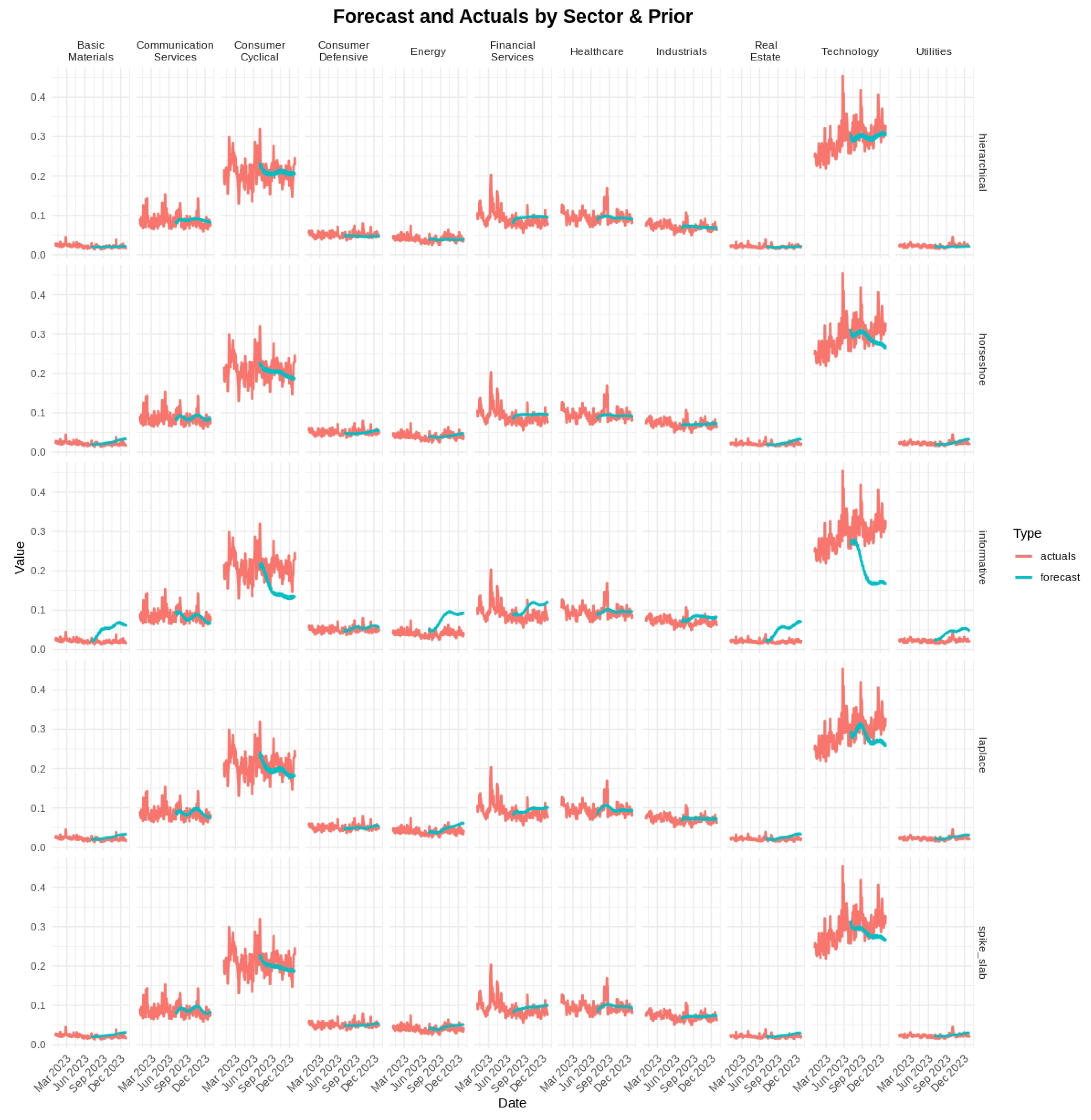
In Figure 5, the forecasts (in turquoise) are shown together with the actual daily proportions (in red) for each sector over the 126-day test interval. The hierarchical and horseshoe priors led to predictions that aligned more closely with the observed values than the informative prior, particularly in volatile sectors such as Energy and Technology. Under the spike-and-slab prior, smaller signals were at times set to zero, which occasionally delayed responses to abrupt shifts in sector composition.
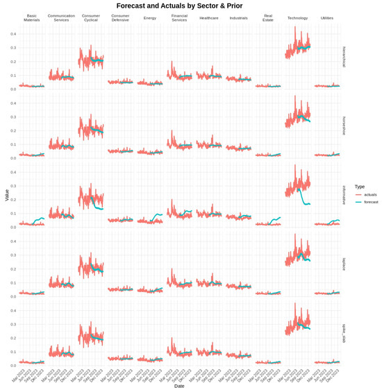
Figure 5.
Forecast and actuals by sector and prior for S&P 500 data. Red lines indicate actual daily sector proportions; turquoise lines are the forecasts from the fitted B-DARMA model. The horseshoe and hierarchical priors tend to track actual series more tightly than the informative prior in many sectors.
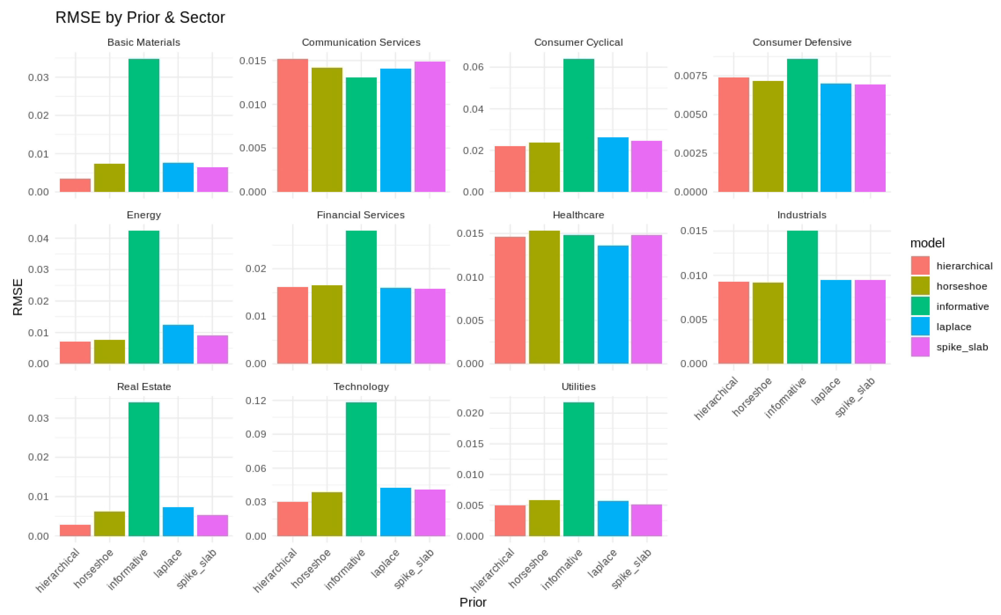
The sector-level RMSE values under each prior are shown in Figure 6, and the average RMSE and MAE values are listed in Table 7. The hierarchical and spike-and-slab priors yielded the smallest RMSE in multiple sectors, and horseshoe priors were found to be effective for larger fluctuations in the Consumer Cyclical and Financial Services sectors. The informative prior generally had higher errors, reflecting the value of regularization in a high-dimensional parameter space.

Figure 6.
RMSE by prior and sector for S&P 500 forecasting. Each facet shows one sector’s RMSE across the five priors.
Table 7.
Mean RMSE and MAE by model for the S&P 500 analysis. We aggregate forecast errors across all 11 sectors under each prior. Lower RMSE and MAE values indicate better overall predictive performance, revealing that the hierarchical and horseshoe strategies often outperform the more permissive informative prior.
Summary of Findings
The findings in this real-data application align with our earlier simulation results. In the large-scale B-DARMA model, shrinkage priors reduced extraneous complexity and lowered forecast errors. The horseshoe, Laplace, and spike-and-slab priors limited the number of active coefficients and delivered stable predictions. Hierarchical priors performed similarly, in part because they partially pool information across related parameters, shrinking them toward a common distribution while still allowing differences where the data support them. Sectors with higher volatility, such as Technology, Communication Services, and Consumer Cyclical, appeared to benefit most from strong shrinkage, whereas more stable sectors like Utilities and Basic Materials performed comparably under all priors. Overall, these outcomes highlight the value of effective regularization in models with multiple lags and complex seasonality, especially in markets that experience rapid fluctuations.
6. Discussion
6.1. Comparisons Across Simulations and Real Data
Our three simulation studies demonstrated how prior selection interacts with model specification in B-DARMA. When the model order matched the true data-generating process (DARMA(2,1)), all priors yielded acceptable results, although the horseshoe and hierarchical priors produced slightly lower RMSE and better interval coverage. Overfitting by fitting B-DARMA(4,2) confirmed that strong shrinkage—particularly the horseshoe—helps suppress spurious higher-order coefficients and avoids inflating forecast errors. Conversely, underfitting remains impervious to prior choice, as omitting critical AR(2) and MA(1) terms led to uniformly higher biases and coverage shortfalls across all priors. All four shrinkage priors neutralized redundant lags, and any of them is preferable to an under-specified alternative.
These lessons translate directly to real data, where we intentionally specified a large-lag B-DARMA model for S&P 500 sector trading. Just as in the overfitting simulation, the horseshoe, Laplace, and spike-and-slab priors effectively shrank extraneous parameters and preserved forecast accuracy. Hierarchical priors provided comparably strong performance through partial pooling, whereas the informative prior yielded higher forecast errors in volatile sectors such as Energy and Technology. These empirical patterns mirror the simulation findings, reinforcing that the combination of a potentially over-parameterized model and minimal shrinkage can lead to unstable estimates and suboptimal forecasts.
Computation time. Using identical Stan settings (four chains, 1250 iterations, 500 warm-ups), the informative prior completed the fastest in about 10 min per chain and served as our baseline. Laplace added roughly 20 % to the wall-clock time (12 min), reflecting the heavier double-exponential tails that require more leapfrog steps. The horseshoe and hierarchical priors were slower by 40 % (14–15 min) because their global–local scale hierarchies force smaller step sizes during HMC integration. Spike-and-slab was the clear outlier, nearly doubling run-time (20 min) owing to the latent inclusion indicators that create funnel-shaped geometry. Practitioners with tight computational budgets might prefer the Laplace prior, while more aggressive sparsity (horseshoe, hierarchical, and spike-and-slab) simply warrants proportionally longer runs.
6.2. Implications and Guidelines
Overall, our results underscore three main points relevant to both simulated and real-world compositional time-series modeling:
- Shrinkage priors mitigate overfitting. Horseshoe priors are especially adept at handling sparse dynamics and large parameter spaces, as shown by the minimal performance degradation in both the simulated and real overfitting scenarios.
- Hierarchical priors offer robust partial pooling. They attain performance comparable to the horseshoe prior while retaining smooth shrinkage across correlated parameters, making them a flexible choice for multi-sector or multi-component series.
- Model misspecification overshadows prior advantages. Underfitting in simulations, or failing to include essential lags in practice, leads to systematic bias and reduced coverage that shrinkage alone cannot remedy. Model identification and appropriate lag selection remain critical for accurate inference.
The S&P 500 data analysis underscores these points: the shrinkage priors consistently outperformed the informative prior in managing a high-dimensional model, yet sector-specific volatility still caused reduced accuracy. Sectors with greater day-to-day variability, such as Technology or Consumer Cyclical, benefited more from aggressive regularization than stable ones (e.g., Utilities and Basic Materials).
Incorporating a dynamic selection of lag structures or exploring alternative priors may further improve compositional forecasting in settings with complex seasonalities or extremely large parameter spaces. Meanwhile, practitioners should pair robust prior modeling with careful model diagnostics (e.g., residual checks and information criteria) to ensure that underfitting and overfitting are detected early.
Overall, these findings reinforce the need for carefully chosen priors, especially in high-dimensional compositional time-series contexts. The horseshoe, Laplace, and hierarchical priors successfully protect against overfitting while preserving essential signals, as illustrated by both the simulation and real-data (S&P 500) analyses. Nonetheless, fundamental model adequacy remains paramount, as even the best prior cannot rescue a structurally under-specified model. We recommend that analysts combine thorough sensitivity checks of priors with well-informed decisions about lag order, covariate inclusion, and potential seasonal effects in B-DARMA applications.
Code Availability
All R analysis scripts and Stan model files are publicly archived at https://github.com/harrisonekatz/bdarma_sensitivity_analysis (accessed on 15 June 2025) (snapshot main@18Jun2025).
Supplementary Materials
The following supporting information can be downloaded at https://www.mdpi.com/article/10.3390/forecast7030032/s1: Table S1. Parameter Estimation Summary for Simulation Study 4 (Correct Specification); Table S2. Parameter Estimation Summary for Simulation Study 5 (Overfitting); Table S3. Parameter Estimation Summary for Simulation Study 6 (Underfitting); Table S4. Forecast Performance Summary Across Supplementary Simulations; Table S5. Forecasting Performance Ratios for Mean RMSE and SD RMSE; Table S6. Forecasting Performance Ratios Within Simulations (Best Model as Denominator).
Author Contributions
Conceptualization, H.K. and R.E.W.; methodology, H.K.; software, H.K. and L.M.; validation, H.K. and L.M.; formal analysis, H.K.; investigation, H.K. and L.M.; data curation, L.M.; writing—original draft preparation, H.K. and L.M.; writing—review and editing, H.K., L.M. and R.E.W.; visualization, H.K.; supervision, R.E.W.; project administration, H.K.; All authors have read and agreed to the published version of the manuscript.
Funding
This research received no external funding.
Data Availability Statement
Raw market data were downloaded from the open-access **“S&P 500 Stocks”** dataset by Andrew Mvd on Kaggle (https://www.kaggle.com/datasets/andrewmvd/sp-500-stocks?select=sp500_stocks.csv; accessed 1 January 2025). Processed sector-share matrices derived from these CSV files are stored in data_analysis/ within the GitHub archive. No new data were created or analysed beyond these publicly available sources; all Monte-Carlo outputs can be regenerated by rerunning the scripts with their fixed random-number seeds.
Conflicts of Interest
Author Harrison Katz and Liz Medina were employed by the company Airbnb. The remaining authors declare that the research was conducted in the absence of any commercial or financial relationships that could be construed as a potential conflict of interest.
References
- Boonen, T.J.; Guillén, M.; Santolino, M. Forecasting compositional risk allocations. Insur. Math. Econ. 2019, 84, 79–86. [Google Scholar] [CrossRef]
- Lipsmeyer, C.S.; Philips, A.Q.; Rutherford, A.; Whitten, G.D. Comparing Dynamic Pies: A Strategy for Modeling Compositional Variables in Time and Space. Political Sci. Res. Methods 2019, 7, 523–540. [Google Scholar] [CrossRef]
- Aitchison, J. The Statistical Analysis of Compositional Data; Chapman and Hall: London, UK, 1986. [Google Scholar]
- Greenacre, M. Compositional Data Analysis in Practice; Chapman and Hall/CRC: New York, NY, USA, 2018; pp. 1–120. ISBN 978-0-429-45553-7. [Google Scholar] [CrossRef]
- Zheng, T.; Chen, R. Dirichlet ARMA models for compositional time series. J. Multivar. Anal. 2017, 158, 31–46. [Google Scholar] [CrossRef]
- Casarin, R.; Grassi, S.; Ravazzolo, F.; Van Dijk, H.K. A Bayesian Dynamic Compositional Model for Large Density Combinations in Finance; Discussion Paper 21-016/III; Tinbergen Institute: Amsterdam, The Netherlands, 2021; pp. 1–51. Available online: https://papers.ssrn.com/sol3/papers.cfm?abstract_id=3783342 (accessed on 17 June 2025).
- Makgai, S.; Bekker, A.; Arashi, M. Compositional Data Modeling through Dirichlet Innovations. Mathematics 2021, 9, 2477. [Google Scholar] [CrossRef]
- Dong, Z.; Shang, H.L.; Hui, F.; Bruhn, A. A compositional approach to modelling cause-specific mortality with zero counts. Ann. Actuar. Sci. 2025, 1–26. [Google Scholar] [CrossRef]
- Katz, H.; Brusch, K.T.; Weiss, R.E. A Bayesian Dirichlet auto-regressive moving average model for forecasting lead times. Int. J. Forecast. 2024, 40, 1556–1567. [Google Scholar] [CrossRef]
- Griffin, J.E.; Brown, P.J. Bayesian global-local shrinkage methods for regularisation in the high-dimensional linear model. Chemom. Intell. Lab. Syst. 2021, 210, 104255. [Google Scholar] [CrossRef]
- Bitto, A.; Frühwirth-Schnatter, S. Achieving shrinkage in a time-varying parameter model framework. J. Econom. 2019, 210, 75–97. [Google Scholar] [CrossRef]
- Mitchell, T.J.; Beauchamp, J.J. Bayesian Variable Selection in Linear Regression. J. Am. Stat. Assoc. 1988, 83, 1023–1032. [Google Scholar] [CrossRef]
- Follett, L.; Yu, C. Achieving parsimony in Bayesian vector autoregressions with the horseshoe prior. Econom. Stat. 2019, 11, 130–144. [Google Scholar] [CrossRef]
- Park, T.; Casella, G. The Bayesian Lasso. J. Am. Stat. Assoc. 2008, 103, 681–686. [Google Scholar] [CrossRef]
- Carvalho, C.M.; Polson, N.G.; Scott, J.G. The Horseshoe Estimator for Sparse Signals. Biometrika 2010, 97, 465–480. [Google Scholar] [CrossRef]
- Polson, N.G.; Sokolov, V. Bayesian regularization: From Tikhonov to horseshoe. Wiley Interdiscip. Rev. Comput. Stat. 2019, 11, e1463. [Google Scholar] [CrossRef]
- Polson, N.G.; Scott, J.G. Local Shrinkage Rules, Lévy Processes and Regularized Regression. J. R. Stat. Soc. Ser. B Stat. Methodol. 2012, 74, 287–311. [Google Scholar] [CrossRef]
- Stan Development Team. RStan: The R Interface to Stan, R Package Version 2.32.7; Stan Development Team: New York, NY, USA, 2025. Available online: https://mc-stan.org/rstan/ (accessed on 17 June 2025).
- Gelman, A.; Carlin, J.B.; Stern, H.S.; Dunson, D.B.; Vehtari, A.; Rubin, D.B. Bayesian Data Analysis, 4th ed.; CRC Press: Boca Raton, FL, USA, 2020. [Google Scholar]

Disclaimer/Publisher’s Note: The statements, opinions and data contained in all publications are solely those of the individual author(s) and contributor(s) and not of MDPI and/or the editor(s). MDPI and/or the editor(s) disclaim responsibility for any injury to people or property resulting from any ideas, methods, instructions or products referred to in the content. |
© 2025 by the authors. Licensee MDPI, Basel, Switzerland. This article is an open access article distributed under the terms and conditions of the Creative Commons Attribution (CC BY) license (https://creativecommons.org/licenses/by/4.0/).