Forecasting Thailand’s Transportation CO₂ Emissions: A Comparison among Artificial Intelligent Models

Abstract

Transportation significantly influences greenhouse gas emissions—particularly carbon dioxide (CO₂)—thereby affecting climate, health, and various socioeconomic aspects. Therefore, in developing and implementing targeted and effective policies to mitigate the environmental impacts of transportation-related carbon dioxide emissions, governments and decision-makers have focused on identifying methods for the accurate and reliable forecasting of carbon emissions in the transportation sector. This study evaluates these policies’ impacts on CO₂ emissions using three forecasting models: ANN, SVR, and ARIMAX. Data spanning the years 1993–2022, including those on population, GDP, and vehicle kilometers, were analyzed. The results indicate the superior performance of the ANN model, which yielded the lowest mean absolute percentage error (MAPE = 6.395). Moreover, the results highlight the limitations of the ARIMAX model; particularly its susceptibility to disruptions, such as the COVID-19 pandemic, due to its reliance on historical data. Leveraging the ANN model, a scenario analysis of trends under the “30@30” policy revealed a reduction in CO₂ emissions from fuel combustion in the transportation sector to 14,996.888 kTons in 2030. These findings provide valuable insights for policymakers in the fields of strategic planning and sustainable transportation development.

1. Introduction

Greenhouse gases (GHGs) are a group of gases that trap heat in the Earth’s atmosphere, leading to the so-called greenhouse effect and contributing to global warming and climate change. Carbon dioxide (CO₂) produced as a result of human activities is the primary cause of global warming among these gases. The past decade (2011–2020) has been the hottest in recorded history [1]. Furthermore, CO₂ levels in the past decade have also increased at historically high rates—rising more than 2 ppm per year—indicating a continuous increase in CO₂ [2]. The increasing amounts of carbon emissions have various environmental impacts, including heatwaves, droughts, floods, storms, and more frequent and severe weather events [3]. These events significantly affect ecosystems, human health, agriculture, and the global economy; leading to concerns about mitigating global climate change and ensuring environmental sustainability [4]. At the same time, countries around the world are striving to reduce GHG emissions and promote sustainable development. The Paris Agreement, which is subsumed under the United Nations Framework Convention on Climate Change, is a significant international accord that reflects global efforts to address climate change. The main goals of the Paris Agreement are: (1) to limit global warming to below 2 degrees Celsius above pre-industrial levels and (2) to pursue continued efforts to limit the temperature increase to 1.5 degrees Celsius.

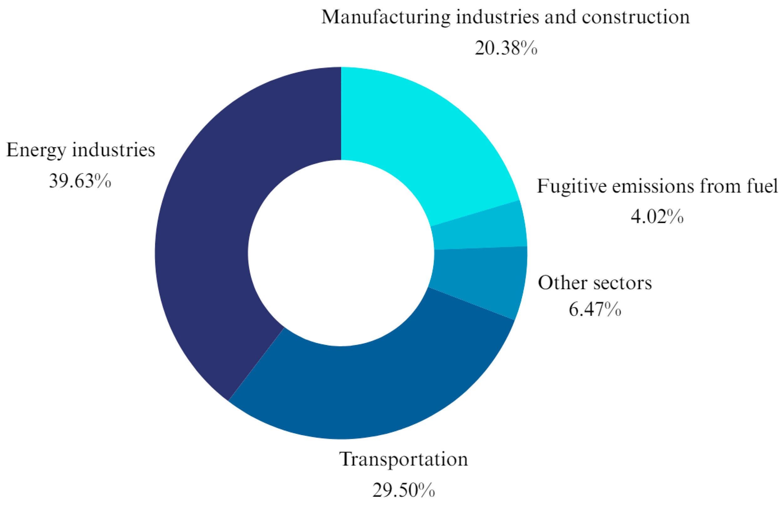
As one of the parties to the agreement, Thailand is also engaged in these global efforts. From 2011 to 2021, the average temperature in the country increased by 0.09 degrees Celsius per year. In 2018, the majority of GHG emissions in the energy sector resulted from fuel combustion [5]. As shown in Figure 1, the Thai transportation sector plays a significant role in producing carbon emissions, contributing to 29.50% of GHG emissions; making it second only to the energy industry, which contributes 39.63% [6]. Therefore, given this background, governments and decision-makers must find accurate and reliable methods of forecasting carbon emissions in the transportation sector; such methods are essential in developing and implementing targeted and effective policies to mitigate the environmental impacts of transportation-related CO₂ emissions [7].

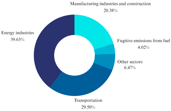
Figure 1. Thailand’s GHG emissions in the energy sector in 2019. Source: Thailand [6].

Various techniques have been employed in the past decade to forecast carbon emissions, ranging from traditional statistical methods to machine learning (ML) algorithms. Previous research has compared CO₂-emission-forecasting models in various contexts. For instance, Ağbulut [8] compared deep learning (DL), support vector machine (SVM), and artificial neural network (ANN) models for forecasting CO₂ emissions in Turkey. To forecast energy demand in the Turkish transportation sector, Sahraei et al. [9] used the multivariate adaptive regression splines (MARS) technique. Tawiah et al. [10] compared autoregressive integrated moving average (ARIMA), nonlinear autoregressive (NAR), exponential smoothing (ETS), naïve approach, and ANN models to forecast CO₂ emissions in Pakistan. Meanwhile, Ning et al. [11] forecasted CO₂ emissions and analyzed future CO₂ emission trends in China using ARIMA. Xu et al. [12] used nonlinear autoregressive exogenous (NARX) to examine the increasing trend of CO₂ emissions in China and analyzed the forecast results using scenario analysis. Liu et al. [13] forecasted energy use in China by comparing multiple linear regression (MLR), a gated recurrent unit artificial neural network (GRU ANN), and support vector regression (SVR). Sun and Liu [14] developed three models—namely, an ANN, an SVM, and the Grey model (GM)—for forecasting CO₂ emissions in China. Thabani and Bonga [15] attempted to model and forecast CO₂ emissions in India using ARIMA. Meanwhile, Fatima et al. [16] studied the relationships of CO₂ gas data in nine Asian countries—namely, Japan, Bangladesh, China, Pakistan, India, Sri Lanka, Iran, Singapore, and Nepal—by comparing the simple exponential smoothing (SES) and ARIMA models; with each country having different suitable models.

Amidst the current landscape of CO₂ forecasting in Thailand, several studies have contributed valuable insights using different modeling techniques. For example, Ratanavaraha and Jomnonkwao [17] forecasted the CO₂ amount released from transportation energy consumption in Thailand by conducting a comprehensive comparison of modeling techniques, including log-linear regression, path analysis, ARIMA, and curve estimation models; considering related factors, such as GDP, population, and the number of registered vehicles. They concluded that the ARIMA model outperformed the others in terms of predictive accuracy. Similarly, Sutthichaimethee and Ariyasajjakorn [18] attempted to forecast CO₂ emissions from industrial energy use in Thailand using the autoregressive integrated moving average with exogenous variables (ARIMAX) model, incorporating GDP and population data into their analysis. In 2022, Salangam [19] proposed an effective and suitable method for forecasting CO₂ levels in Thailand by comparing regression analysis and an ANN; this incorporated variables such as GDP, population, energy consumption, and the number of registered vehicles. Their results indicated that the ANN predictions of CO₂ levels were six times more efficient and accurate than those derived from regression analysis methods. By demonstrating improved efficiency and accuracy over traditional regression techniques, such a finding suggests that ANNs hold promise as a superior tool for CO₂ forecasting in the context of Thailand. To systematically present relevant research results and provide a comprehensive perspective on analytical methods, we categorized studies by author, methods used, input and output variables, and the region each study pertains to; as shown in Table 1.

CO₂ forecasting faces several limitations, including the complexity of the drivers of emissions (e.g., economic activity, technology, and policies) and the uncertainty and variability of emissions and external shocks, such as natural disasters, the COVID-19 pandemic, and geopolitical events, among others. Furthermore, limited data availability can lead to violations of the statistical assumptions required for some forecasting methods. The most common methods for forecasting carbon emissions are ANN, ARIMA, and SVR, which have different strengths and weaknesses when dealing with forecasting problems. ANNs, in particular, are highly flexible and can adapt to various types of data patterns, including those involving nonlinear relationships [20] or violations of traditional statistical assumptions, such as normality (to some extent) [21]. SVR is also adept at capturing nonlinear relationships [22] and is less affected by outliers than traditional regression methods. ARIMAX—or ARIMA with exogenous variables—allows it to account for external factors or intervention events that may influence time series data, thereby improving forecasting accuracy [23,24,25]. However, compared with simpler models such as ARIMAX, ANN and SVR models can be very complex and challenging to interpret. To date, no studies have compared the performance of these three methods in forecasting transportation-related CO₂ emissions in Thailand. Therefore, the current study aims to fill this gap by providing a comprehensive comparison of ANN, ARIMAX, and SVR models in this context.

First, we review the theoretical foundations of each technique. Then, we assess the performance of these models on past carbon emission datasets using various evaluation metrics; including root mean square error (RMSE), mean absolute error (MAE), and mean absolute percentage error (MAPE). Finally, we provide insights into the appropriateness of using these models for forecasting carbon emissions and suggest future research directions to enhance their predictive capabilities.

Table 1. Summary of studies on emission forecasting found in the literature review.

Authors	Method	Region	Input Variable	Output Variable	Performance Evaluation
Salangam [19]	Regression, ANN *	Thai	GDP, population, energy consumption, number of registered vehicles	CO2	MAD, R-squared
Ağbulut [8]	DL, SVM *, ANN	Turkey	GDP, population, vehicle-km	CO2	R-squared, RMSE, MAPE, MBE, MABE
Ning, Pei, and Li [11]	ARIMA	China	Previous CO2 data	CO2	R-squared, AIC, SC
Fatima, Saad, Zia, Hussain, Fraz, Mehwish, and Khan [16]	SES, ARIMA	Japan, Iran, Bangladesh, China, Pakistan, India, Sri Lanka, Singapore, Nepal	Previous CO2 data	CO2	FMAE
Xu, Schwarz, and Yang [12]	NARX	China	Industrialization rate, urbanization rate, GDP, proportions of industry and service sectors, proportions of tertiary sector, population, energy consumption	CO2	MAE
Ratanavaraha and Jomnonkwao [17]	log-linear regression, path analysis, ARIMA *, curve estimation	Thailand	GDP, population, number of small-sized registered vehicles, number of medium-sized registered vehicles, number of large-sized registered vehicles	CO2	R-squared, MSE, MAPE
Sahraei, Duman, Çodur, and Eyduran [9]	MARS	Turkey	GDP, oil price, population, ton-km, vehicle-km, passenger-km	Transport energy demand	GR-squared, R-squared, adjust R-squared, RMSE, AIC
Tawiah, Daniyal, and Qureshi [10]	ARIMA, ETS, Naïve Approach, MLP, NAR *	Pakistan	Previous CO2 data	CO2	RMSE, MAE
Sutthichaimethee and Ariyasajjakorn [18]	ARIMAX	Thai	Population, GDP	CO2	R-squared
Liu, Fu, Bielefield, and Liu [13]	MLR, SVR, GRU ANN *	China	GDP, population, population, import trade volume, export trade volume	CO2	MAPE, RMSE
Thabani and Bonga [15]	ARIMA	India	Previous CO2 data	CO2	AIC, MAE, RMSE, MAPE
Sun and Liu [14]	LSSVM *, GM, ANN, Logistic Model	China	Factors related to major industries and household consumption such as GDP, passenger traffic, urban population, and total retail sales of consumer products	CO2	MAPE, RMSE, MaxAPE, MdAPE
Ghalandari et al. [26]	GMDH, ANN *	UK, Germany, Italy, France	GDP, oil consumption, coal, natural gas, nuclear energy, renewable energy consumption	CO2	R-squared, MSE
Faruque et al. [27]	LSTM, CNN, CNN-LSTM, DNN *	Bangladesh	GDP, electrical energy consumption	CO2	MAPE, RMSE, MAE,
Shabri [28]	GM, ANN, GMDH, Lasso-GMDH *	Malaysia	Population, GDP, energy consumption, number of registered motor vehicles, amount invested	CO2	MAPE
Rahman and Hasan [29]	ARIMA	Bangladesh	Previous CO2 data	CO2	RMSE, MAE, MPE, MAPE, MASE, AIC, BIC
Kour [30]	ARIMA	South Africa	Previous CO2 data	CO2	RMSE
Kamoljitprapa and Sookkhee [31]	ARIMA	Thailand	Previous CO2 data	CO2	R-squared, adjusted R-squared, AIC
Zhu et al. [32]	SVR	China	Population, GDP, urbanization rate, energy consumption structure, energy intensity, industrial structure	CO2	MSE
Li et al. [33]	GM, DGM, RDGM ARIMA *	China	Previous CO2 data, GDP	CO2	MAPE
Yang et al. [34]	SVR	China	GDP, coal, coke, gasoline, diesel oil, crude oil, kerosene, fuel oil, and natural gas consumption	CO2	MAPE

* Indicates the best-performing model among those compared in a study.

Table 1. Summary of studies on emission forecasting found in the literature review.

Authors	Method	Region	Input Variable	Output Variable	Performance Evaluation
Salangam [19]	Regression, ANN *	Thai	GDP, population, energy consumption, number of registered vehicles	CO2	MAD, R-squared
Ağbulut [8]	DL, SVM *, ANN	Turkey	GDP, population, vehicle-km	CO2	R-squared, RMSE, MAPE, MBE, MABE
Ning, Pei, and Li [11]	ARIMA	China	Previous CO2 data	CO2	R-squared, AIC, SC
Fatima, Saad, Zia, Hussain, Fraz, Mehwish, and Khan [16]	SES, ARIMA	Japan, Iran, Bangladesh, China, Pakistan, India, Sri Lanka, Singapore, Nepal	Previous CO2 data	CO2	FMAE
Xu, Schwarz, and Yang [12]	NARX	China	Industrialization rate, urbanization rate, GDP, proportions of industry and service sectors, proportions of tertiary sector, population, energy consumption	CO2	MAE
Ratanavaraha and Jomnonkwao [17]	log-linear regression, path analysis, ARIMA *, curve estimation	Thailand	GDP, population, number of small-sized registered vehicles, number of medium-sized registered vehicles, number of large-sized registered vehicles	CO2	R-squared, MSE, MAPE
Sahraei, Duman, Çodur, and Eyduran [9]	MARS	Turkey	GDP, oil price, population, ton-km, vehicle-km, passenger-km	Transport energy demand	GR-squared, R-squared, adjust R-squared, RMSE, AIC
Tawiah, Daniyal, and Qureshi [10]	ARIMA, ETS, Naïve Approach, MLP, NAR *	Pakistan	Previous CO2 data	CO2	RMSE, MAE
Sutthichaimethee and Ariyasajjakorn [18]	ARIMAX	Thai	Population, GDP	CO2	R-squared
Liu, Fu, Bielefield, and Liu [13]	MLR, SVR, GRU ANN *	China	GDP, population, population, import trade volume, export trade volume	CO2	MAPE, RMSE
Thabani and Bonga [15]	ARIMA	India	Previous CO2 data	CO2	AIC, MAE, RMSE, MAPE
Sun and Liu [14]	LSSVM *, GM, ANN, Logistic Model	China	Factors related to major industries and household consumption such as GDP, passenger traffic, urban population, and total retail sales of consumer products	CO2	MAPE, RMSE, MaxAPE, MdAPE
Ghalandari et al. [26]	GMDH, ANN *	UK, Germany, Italy, France	GDP, oil consumption, coal, natural gas, nuclear energy, renewable energy consumption	CO2	R-squared, MSE
Faruque et al. [27]	LSTM, CNN, CNN-LSTM, DNN *	Bangladesh	GDP, electrical energy consumption	CO2	MAPE, RMSE, MAE,
Shabri [28]	GM, ANN, GMDH, Lasso-GMDH *	Malaysia	Population, GDP, energy consumption, number of registered motor vehicles, amount invested	CO2	MAPE
Rahman and Hasan [29]	ARIMA	Bangladesh	Previous CO2 data	CO2	RMSE, MAE, MPE, MAPE, MASE, AIC, BIC
Kour [30]	ARIMA	South Africa	Previous CO2 data	CO2	RMSE
Kamoljitprapa and Sookkhee [31]	ARIMA	Thailand	Previous CO2 data	CO2	R-squared, adjusted R-squared, AIC
Zhu et al. [32]	SVR	China	Population, GDP, urbanization rate, energy consumption structure, energy intensity, industrial structure	CO2	MSE
Li et al. [33]	GM, DGM, RDGM ARIMA *	China	Previous CO2 data, GDP	CO2	MAPE
Yang et al. [34]	SVR	China	GDP, coal, coke, gasoline, diesel oil, crude oil, kerosene, fuel oil, and natural gas consumption	CO2	MAPE

* Indicates the best-performing model among those compared in a study.

2. Materials and Methods

2.1. Data Collection

The data acquired for this study were compiled annually, covering a 30-year period from 1993 to 2022. The dataset comprised CO₂ emissions data from the transportation sector, population, GDP, VK Passenger, VK Freight, and VK Motorcycle. These data were collected from secondary sources provided by various institutions. Detailed sources and information regarding the data are presented in Table 2. These secondary data sources ensured that the information they provided is comprehensive and reliable for analysis. Each agency provides specific datasets relevant to their domain, contributing to a robust and detailed dataset.

Table 2. Variable, data source, and description.

Variable	Source	Description
CO2 (kTons)	EPPO	CO2 emissions from the transportation sector
Population (103 Peoples)	World Bank	Total population is based on the de facto definition of population, which counts all residents regardless of legal status or citizenship. The values shown are midyear estimates.
GDP (109 Baht)	Bank of Thailand	Gross domestic product—chain volume measures.
VK Passenger (106 vehicle-kilometers)	Bureau of Highway Safety, Department of Highways, Thailand	Travel volume in the study area classified by type of vehicle. VK Passenger consists of five vehicle types; namely, passenger cars carrying fewer than seven persons, passenger cars carrying more than seven persons, light buses, medium buses, and heavy buses.
VK Freight (106 vehicle-kilometers)		Travel volume in the study area classified by type of vehicle. VK Freight consists of five vehicle types, including light trucks, medium trucks, heavy trucks, full trailers, and semi-trailers.
VK Motorcycle (106 vehicle-kilometers)		Travel volume in the study area classified by motorcycle.

The data cleaning and preprocessing phase is crucial for ensuring the accuracy and reliability of an analysis. In this study, initially, missing values were addressed through imputation methods, where incomplete records were either filled with appropriate estimates or removed if they were deemed insufficiently representative. The data were then standardized to ensure comparability across different variables. Standardization involved scaling the data such that each variable had a mean of zero and a standard deviation of one. This process helps in normalizing the range of the variables, particularly when they are measured on different scales. Following standardization, outliers were managed using the Z-score method. For each variable, the Z-score is given by the following [35,36]:

$$Z=\frac{\left(X-\mu \right)}{\sigma },$$

(1)

where $X$ is the data point, $\mu$ is the mean, and $\sigma$ is the standard deviation. Data points with Z-scores exceeding the threshold of 3 or −3 were considered outliers [35,37]. These outliers were removed from the dataset or transformed.

Table 3 shows a strong correlation between input and output variables such as population, GDP, annual vehicle kilometers (VK), and historical CO₂ emissions [38]. Therefore, these inputs were utilized in training models to predict CO₂ emissions related to transportation [8].

Table 3. Correlation matrices of the variables.

Variable	Population	GDP	VK Passenger	VK Freight	VK Motorcycle	CO2
Population	1	0.949	0.947	0.914	0.828	0.824
GDP	0.949	1	0.950	0.944	0.870	0.839
VK Passenger	0.947	0.950	1	0.982	0.936	0.837
VK Freight	0.914	0.944	0.982	1	0.953	0.914
VK Motorcycle	0.828	0.870	0.936	0.953	1	0.797
CO2	0.824	0.839	0.837	0.914	0.797	1

2.2. Data Analysis

ANNs are adept at capturing complex, nonlinear relationships; making them suitable models for predicting CO₂ levels in various settings [8,19,26]. SVR, which is known for its efficiency in high-dimensional spaces, can handle nonlinear data effectively and is another widely used ML method for CO₂ level prediction [14,32,34]. ARIMA, a popular statistical approach for forecasting CO₂—as depicted in Table 1—is specifically designed for time series data; analyzing and making predictions based on historical trends. However, we believe that incorporating appropriate exogenous variables into this model can further improve accuracy. Therefore, we employed ARIMAX. Overall, these methods provide a comprehensive toolkit for predicting CO₂ levels; each offering unique strengths with which to address the complexities of data analysis.

2.2.1. Artificial Neural Network

Artificial Neural Networks (ANNs) are a type of machine learning method inspired by the structure and functioning of the human brain. They consist of numerous interconnected processing units called neurons, which collaborate to process information and recognize patterns. The learning process of an ANN involves adjusting weights through a method known as backpropagation. Initially, input data are fed into the network and pass through multiple layers, where each layer applies weights and activation functions to transform the data, ultimately producing the final output. The network’s output is then compared to the actual target values using a loss function, which quantifies the difference between the predicted and actual values. Common loss functions include the mean squared error (MSE) for regression tasks and cross-entropy loss for classification tasks. The error from the loss function is propagated back through the network, and the weights are adjusted to minimize this error by using optimization algorithms such as Gradient Descent. This cycle of forward propagation, loss calculation, and backward propagation continues iteratively until the error is minimized to an acceptable level, allowing the ANN to learn the underlying patterns in the data under analysis.

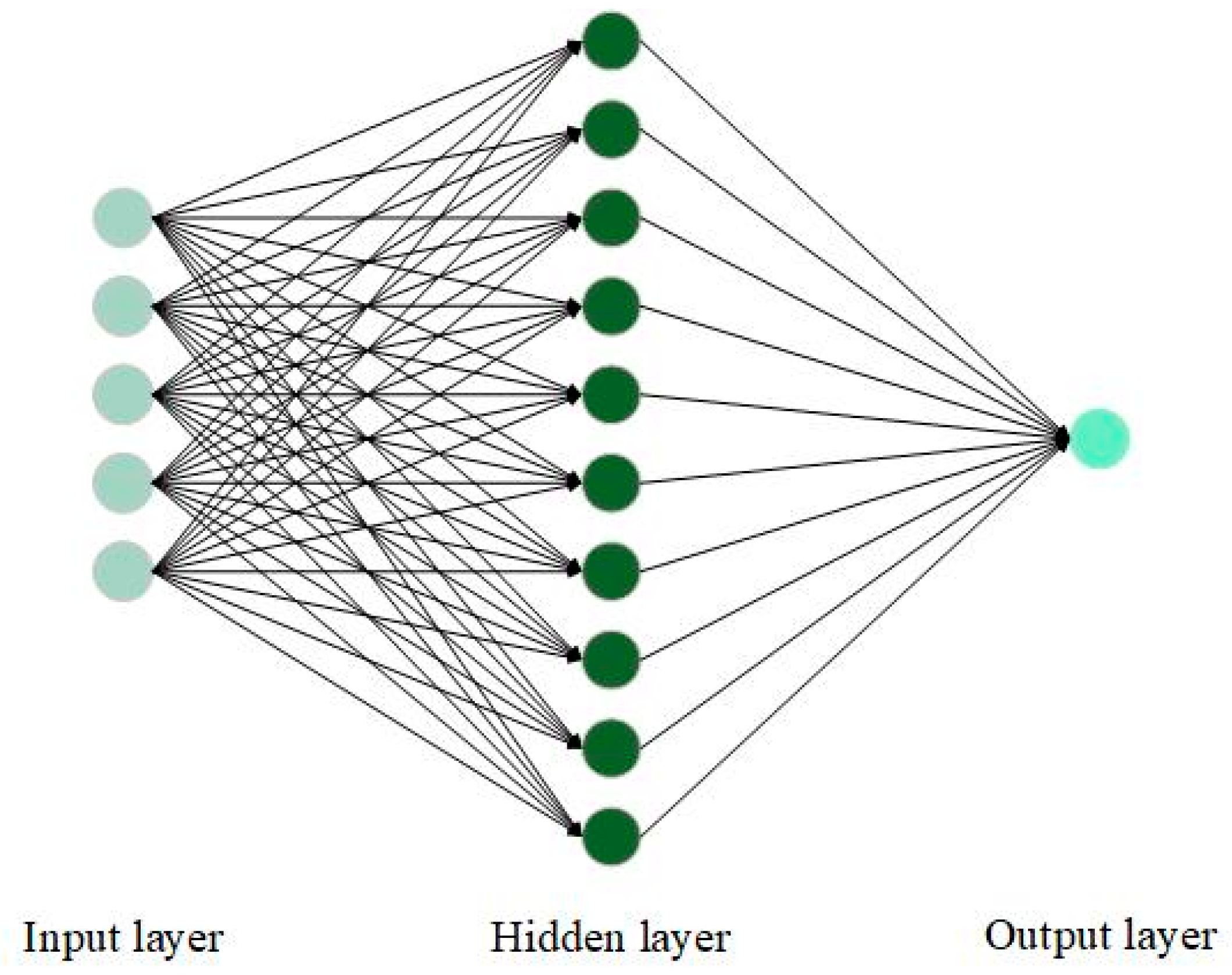
ANN are highly adaptable to various data patterns, including nonlinear relationships [20], and can handle complex data structures that traditional statistical methods may struggle with; for example, the violation of the assumption of normality [21]. However, they also come with inherent complexity and often lack interpretability [39], making it difficult to understand how specific predictions are made. Moreover, ANN typically require large quantities of data and substantial computational power for training. The architecture of an artificial Multi-Layer Perceptron (MLP) neural network is shown in Figure 2. Meanwhile, the mathematical formula for obtaining the forecasting output for the $j^{th}sample$ can be calculated using the following equation [40]:

$$y_j={\displaystyle \sum _{i=1}^n{\omega }_{ki,j}f\left(h_k\right)}+{\beta }_j$$

(2)

where ${\omega }_{ki,j}$ denotes the weights from the $k^{th}$ hidden node to an output node in the $i^{th}$ iteration, ${\beta }_j$ indicates the bias of the $j^{th}$ output node sample, $f\left(h_k\right)$ is the outcome of hidden node $h_k$ after the activation function has been applied, and $y_j$ refers to the output of the $j^{th}$ sample.

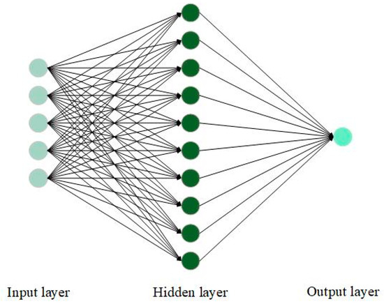
Figure 2. Architecture of an artificial neural network (ANN).

2.2.2. Support Vector Regression

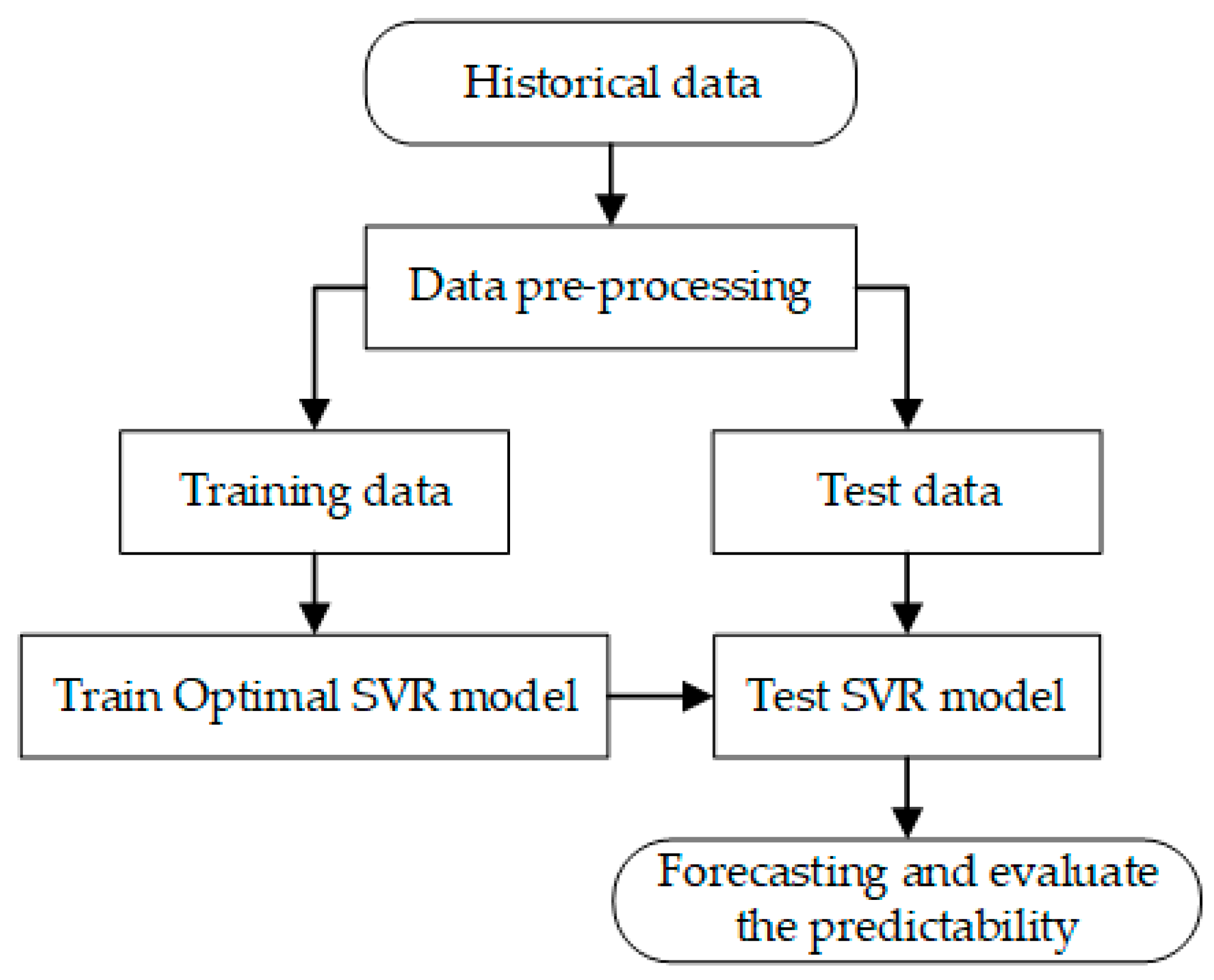
Support vector regression (SVR) is a machine learning method in which techniques from a support vector machine (SVM) are used to predict continuous outcomes. Initially developed for classification tasks, SVMs have been adapted to handle regression problems [41]. SVR is based on the concepts of margin and support vectors. In SVR, the margin refers to the epsilon-insensitive tube around the regression function, within which prediction errors are not penalized. Support vectors are data points that lie on the boundary of this margin or outside it, playing a crucial role in defining the regression function. The decision function of SVR is primarily determined by these support vectors, making SVR generally robust to outliers, depending on the choice of the epsilon parameter [42]. The kernel function is used to map input data to higher-dimensional spaces, enabling SVR to handle nonlinear relationships [43]. Figure 3 displays a flowchart of an SVR approach. An SVR model with a linear kernel is represented as follows [13,44,45]:

$${\widehat{y}}^{SVR}={\displaystyle {\sum }_{i=1}^m({\alpha }_i-{\alpha }_i^{*})}K(x_i,x_j)+b,$$

(3)

where ${\widehat{y}}^{svr}$, $({\alpha }_i-{\alpha }_i^{*})$, and $b$ represent the output, the difference between the Lagrange multipliers, and the bias, respectively. The kernel function for a linear SVR is denoted by $K(x_i,x_j)$, for which the following holds [45]:

$$K(x_i,x_j)=x_i\cdot x_j$$

(4)

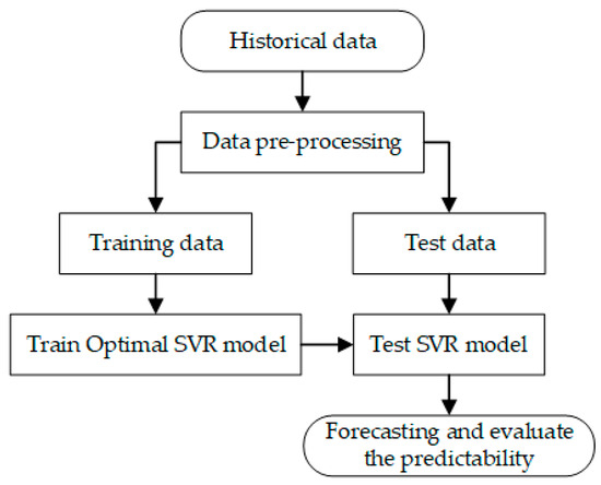
Figure 3. Flowchart of support vector regression (SVR).

2.2.3. Bayesian Optimization

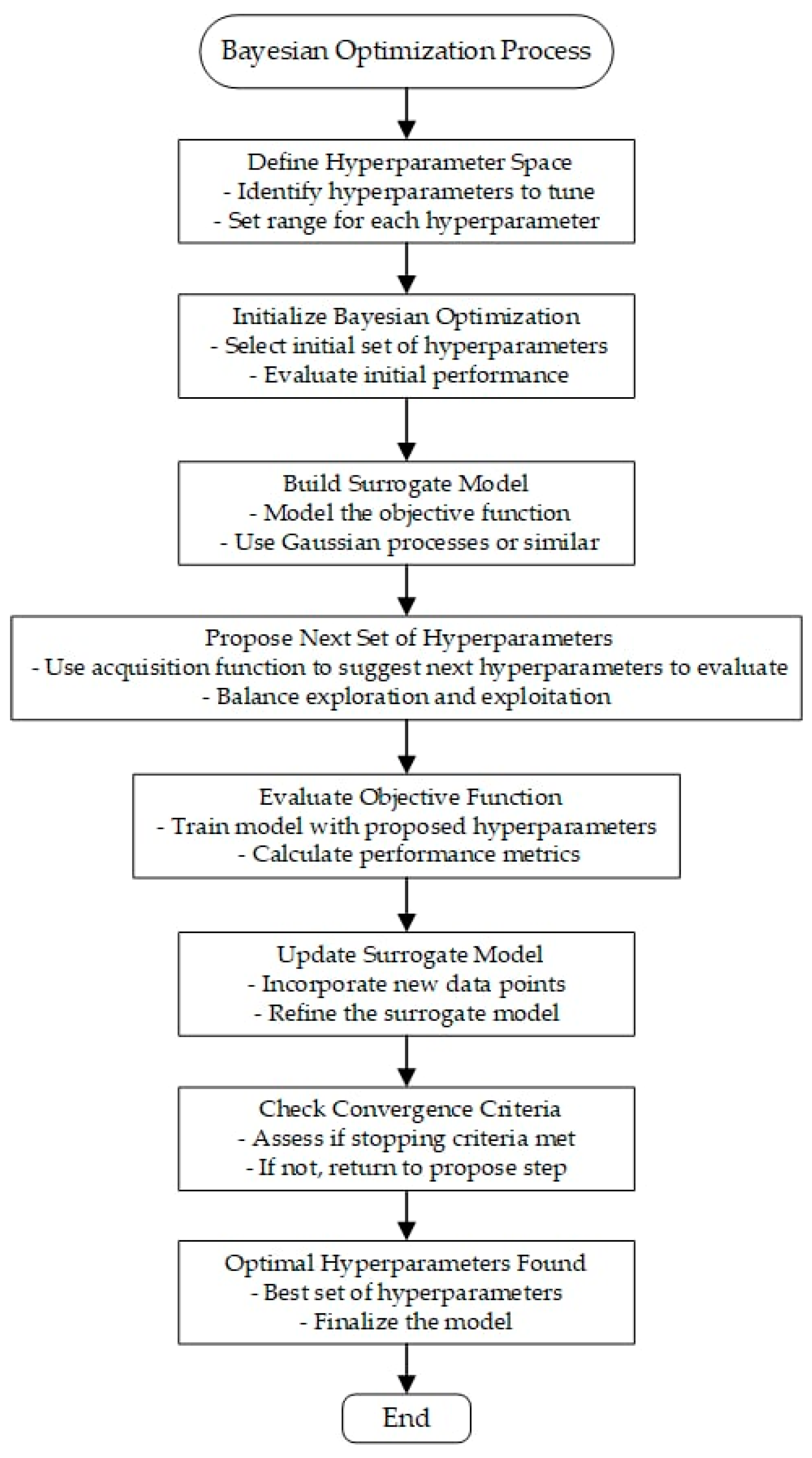
In this study, we employed Bayesian optimization as a strategic method for fine-tuning the hyperparameters of the ML model [46,47]. Bayesian optimization is an effective method for optimizing the hyperparameters of complex models such as ANN and SVR. It efficiently searches the hyperparameter space by building a probabilistic model (surrogate model) of the objective function using past evaluations, making the process more efficient than a grid search or random search [48]. Studies have shown that Bayesian optimization is particularly suitable for hyperparameter tuning—enabling the optimization of black-box functions without requiring analytical expressions or gradients—making it ideal for scenarios where evaluations are expensive and noisy [49,50].

The process of optimizing hyperparameters using Bayesian optimization involves a series of meticulously planned steps, as illustrated in Figure 4. Initially, the hyperparameter space is defined by identifying the hyperparameters that require optimization, and setting their possible ranges or values. These parameters can include the number of layers, the number of neurons per layer, activation functions, learning rate, batch size, and regularization strength.

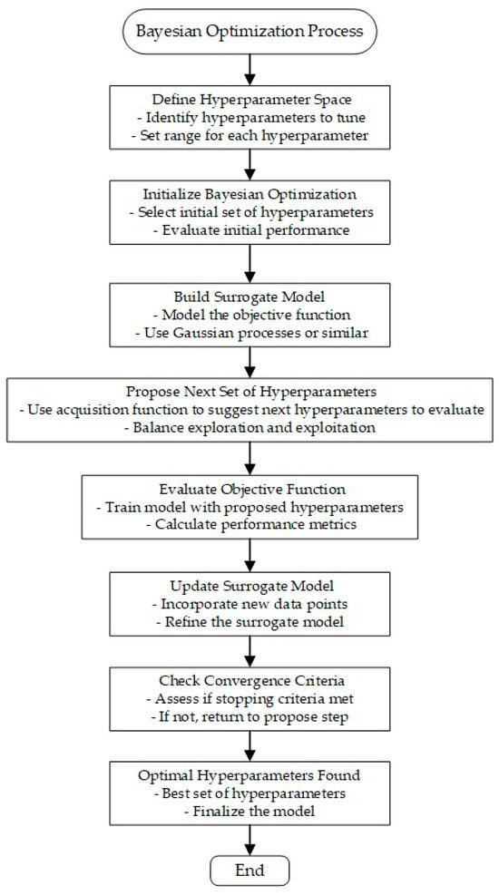
Figure 4. The process of optimizing hyperparameters using Bayesian optimization.

Afterward, Bayesian optimization is initialized by selecting an initial set of hyperparameters. These can be chosen randomly or based on prior knowledge. The model’s performance with these initial settings in place is then evaluated using metrics such as mean squared error (MSE) or root mean squared error (RMSE). Subsequently, a surrogate model—typically a Gaussian process—is constructed to approximate the objective function and predict the performance of various hyperparameter settings.

The next step involves proposing a new set of hyperparameters using an acquisition function. This function strikes a balance between exploring new configurations and exploiting known promising ones. The model is then trained using these proposed hyperparameters, and performance metrics are calculated to assess its effectiveness. The results from these evaluations are integrated into the surrogate model, refining its accuracy and predictive capability.

The next step in the optimization process consists of checking convergence criteria, which may include reaching a maximum number of iterations, achieving convergence in the objective function, or obtaining satisfactory performance improvement. If the stopping criteria are not met, the process returns to proposing the next set of hyperparameters. Once the stopping criteria are satisfied, the optimal set of hyperparameters is identified, and the model is finalized with these optimal parameters for deployment or further testing.

2.2.4. Autoregressive Integrated Moving Average with Exogenous Variables

ARIMA is a statistical model that is used to analyze time series data to forecast future values based on past values [51]. This model decomposes data into three processes: autoregressive (AR), which forecasts a variable based on its past values; integrated (I), which serves to stabilize data or make them stationary; and moving average (MA), which forecasts a variable considering errors at previous points [52]. The components of the model consist of three parameters, represented by integers in the form (p, d, q); where p indicates the Lag order or autoregressive of order p, d indicates the number of times the data are differenced or integrated to make them stationary, and q indicates the Lag order or MA of order q. Time series data can often be influenced by special events such as legislative activities, policy changes, environmental regulations, and other similar events. These are referred to as intervention events. By incorporating appropriate exogenous variables that capture the effects of intervention events, an ARIMAX model can significantly improve forecasting performance [23,24,25]. This approach is particularly useful in contexts wherein external factors are known to influence the time series data. Meanwhile, the mathematical expression for ARIMAX is depicted as Equation (5), which is derived from merging the mathematical expressions of four components: AR, represented by Equation (6); I, represented by Equation (7); MA, illustrated by Equation (8); and Exogenous Variables (X), illustrated by Equation (9) [24,51,53,54].

$${\Delta }^d{Y}_t={\displaystyle \sum _{i=1}^p{\varphi }_i{\Delta }^d{Y}_{t-i}}+{\displaystyle \sum _{j=1}^q{\theta }_j{\epsilon }_{t-j}+{\beta }_k{X}_{tk}+}{\epsilon }_t,$$

(5)

$$Y_t={\varphi }_1{Y}_{t-1}+{\varphi }_2{Y}_{t-2}+\dots +{\varphi }_p{Y}_{t-p}+{\epsilon }_t,$$

(6)

$${\Delta }^d{Y}_t={(1-B)}^d{Y}_t,$$

(7)

$$Y_t={\theta }_1{\epsilon }_{t-1}+{\theta }_2{\epsilon }_{t-2}+\dots +{\theta }_q{\epsilon }_{t-q}+{\epsilon }_t,$$

(8)

$$Y_t={\beta }_1{X}_{t1}+{\beta }_2{X}_{t2}+\dots +{\beta }_k{X}_{tk}$$

(9)

Here, $Y_t$ is the value of the series at the $t^{th}$ time, $\varphi$ denotes the coefficients of the AR part, ${\Delta }^d$ denotes differencing $d$ times, $B$ is the backshift operator, $\theta$ is the coefficient of the MA part, ${\beta }_k$ is the coefficients of the exogenous variables $X_{tk}$, and $\epsilon$ is the white noise error term.

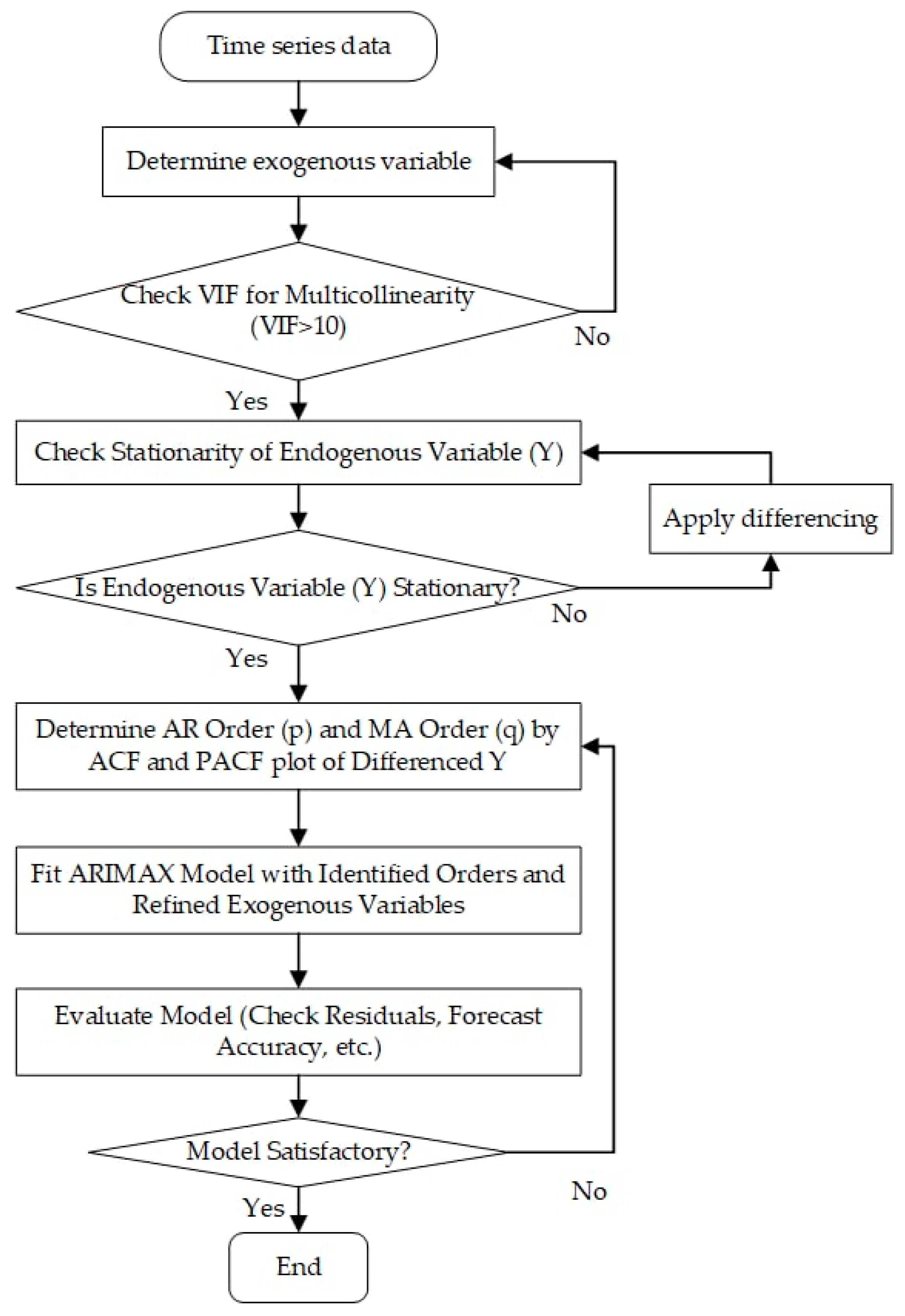
The ARIMAX framework is shown in Figure 5. After loading and preprocessing the data, the next step consists of checking for multicollinearity among exogenous variables using VIF. If high multicollinearity is found, variables are removed or combined. The stationarity of the endogenous variable (Y) is then checked; if it is non-stationary, differencing is applied. Once stationarity is achieved, ACF and PACF plots of the differenced series are used to determine the AR (p) and MA (q) orders. The ARIMAX model is fitted with these orders and the refined exogenous variables. The model is evaluated for residuals and forecast accuracy. If the model is deemed satisfactory, it is used; otherwise, the specification is reevaluated. This process ends once a satisfactory model is obtained.

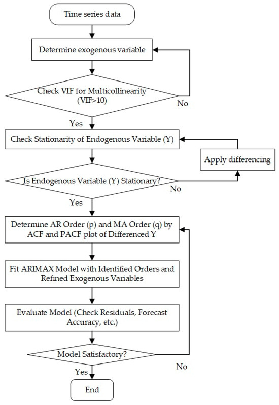
Figure 5. ARIMAX flowchart.

2.2.5. Scenario Analysis

Scenario analysis is a tool used to analyze and assess the impacts that may arise from different events or situations in the future. In particular, this tool is used to assist in decision-making and strategic planning in uncertain or risky conditions. It includes the best case (optimistic scenario), which explores the impacts in a case wherein everything proceeds as well as possible; the worst case (pessimistic scenario), which explores the impacts in a case wherein the worst situation occurs; and the base-case scenario, which explores the impacts in a case where conditions are normal or as expected. The likelihood and possible impacts of these scenarios should be considered alongside strategic planning [55].

2.3. Evaluation Metrics and Statistical Tests

In this study, we utilized three significant statistical measures—RMSE, MAE, and MAPE—to evaluate the efficacy of our model’s forecasting abilities. Each of these metrics offers unique insights into our model’s accuracy and precision. Lower values across these measures indicate better model performance.

RMSE is metric that not only measures the difference between the predicted values and the actual values in a dataset but also evaluates the average magnitude of the prediction errors made by the model. It can be expressed as shown in Equation (7). MAE is a commonly used metric in regard to ML statistics for evaluating the performance of predictive models. MAE measures the average magnitude of errors between the predicted and actual values, as shown in Equation (8). MAPE is a metric that assesses the accuracy of a model’s predictions by measuring the average percentage difference between the predicted and actual values in a dataset, as shown in Equation (9).

$$\mathrm{RMSE}=\sqrt{\frac{{\displaystyle \sum _{i=1}^n{\left(y_i-{\widehat{y}}_i\right)}^2}}{n}}$$

(10)

$$\mathrm{MAPE}=\left(\frac{1}{n}{\displaystyle \sum _{i=1}^n\frac{\left|y_i-{\widehat{y}}_i\right|}{\left|y_i\right|}}\right)\times 100$$

(11)

$$\mathrm{MAE}=\left(\frac{1}{n}\right)\times {\displaystyle \sum _{i=1}^n\left|y_i-{\widehat{y}}_i\right|}$$

(12)

In Equations (10)–(12), $n$ is the total number of observations or data points, $y_i$ represents the actual value of the $i^{th}$ observation, and ${\widehat{y}}_i$ represents the predicted value of the $i^{th}$ observation. In addition, in previous studies [8,56,57,58], the evaluation of the MAPE metric has been categorized into four levels, as shown in Table 4.

Table 4. Guidelines for interpreting the ability of MAPE to forecast accuracy.

MAPE Range	Forecasting Accuracy
≤10%	High prediction accuracy
>10% and ≤20%	Good prediction accuracy
>20% and ≤50%	Reasonable prediction accuracy
>50%	Inaccurate prediction accuracy

In addition to these metrics, the Harvey, Leybourne, and Newbold (HLN) test was employed to statistically compare the predictive accuracy of the models [59]. The HLN test, an extension of the Diebold-Mariano (DM) test, is particularly useful for small sample sizes, providing a more robust test statistic [60,61]. The null hypothesis ($H_0$) of the HLN test posits that there is no difference in the predictive accuracy between two models $(E(d_i)=0)$, where $d_i$ represents the difference in forecast errors between the models. The alternative hypothesis ($H_1$) suggests that there is a significant difference in predictive accuracy $(E(d_i)\ne 0)$. Several studies have successfully applied the HLN test to evaluate forecasting models. For instance, Mizen and Tsoukas [61], Jiao et al. [62], and Song et al. [63] have applied the HLN test to evaluate forecasting models, highlighting the HLN test’s applicability and effectiveness in various forecasting contexts.

3. Results

3.1. Data Descriptive

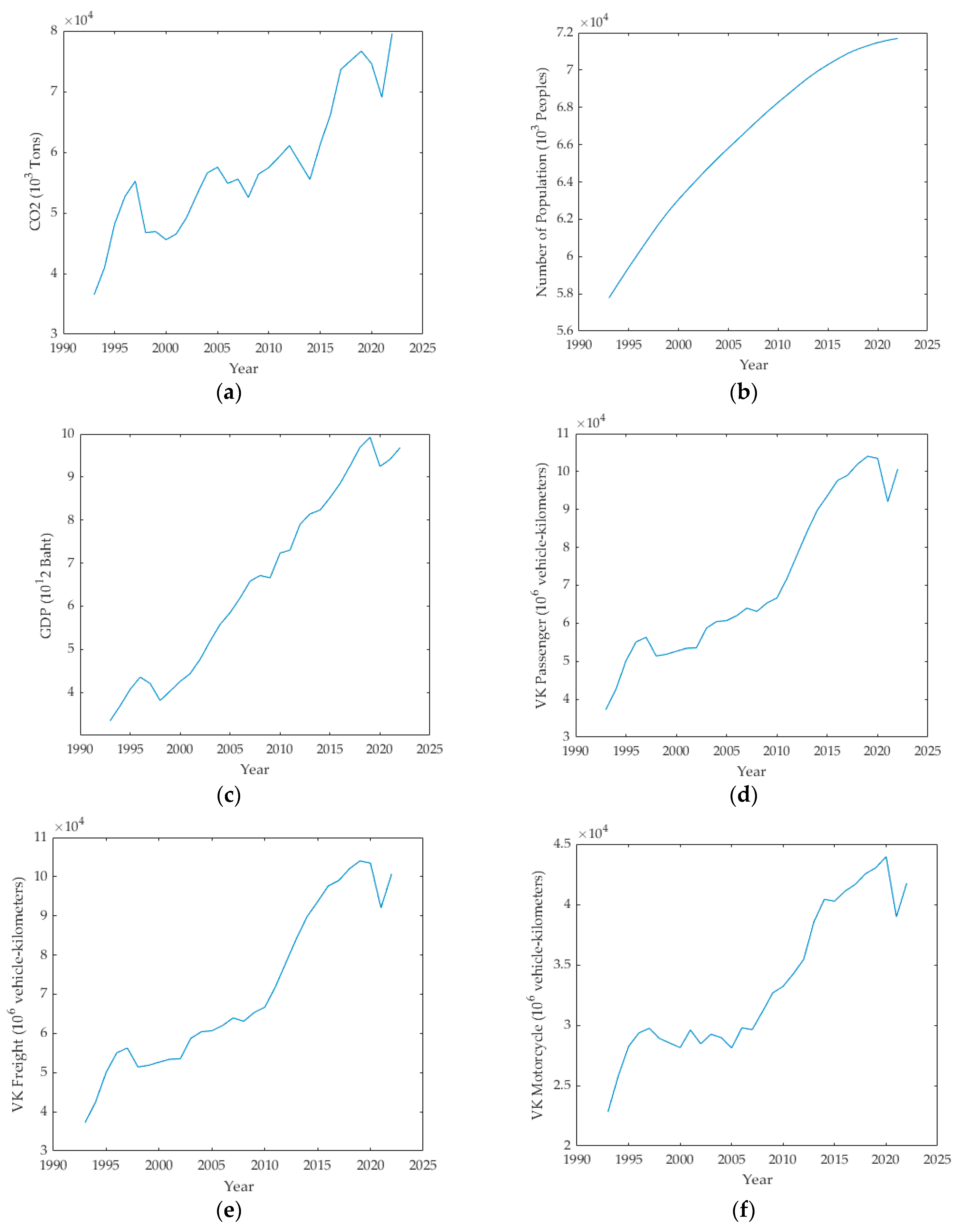
The dataset for forecasting CO₂ emissions in Thailand covers the period from 1993 to 2022. In particular, the current study used data from 1993 to 2013 to train the models, while data from 2014 to 2022 were used to test the models’ performance. The ANN and SVM models used population, GDP, VK Passenger, VK Freight, and VK Motorcycle as input variables, while the ARIMAX model used the previous values of CO₂ emissions as input variables. Figure 6a presents a significant rise in CO₂ emissions from the transportation sector, which peaked around 2022. The data indicate increased vehicular activity and possibly lax emission standards, although there seems to have been a decreasing trend in recent years. Thailand’s demographic dynamics, shown in Figure 6b, illustrate a continuous upward trend, also indicating a stable economic and social environment. Despite such data, the decelerating growth rate in recent years signifies a structural shift toward an aging society. GDP, as depicted in Figure 6c, highlights Thailand’s economic ascendancy, particularly after 2000; with a discernible decrease during the global financial crisis of 2008–2009. Comparable trends can be seen in Figure 6d–f, which illustrate vehicle-kilometers for passenger vehicles, freight, and motorcycles. Furthermore, a notable surge was observed post-2010, which may have been due to economic expansion or increased urbanization. However, the evident decline post-2019 is attributable to travel restrictions stemming from pandemic prevention measures relating to COVID-19.

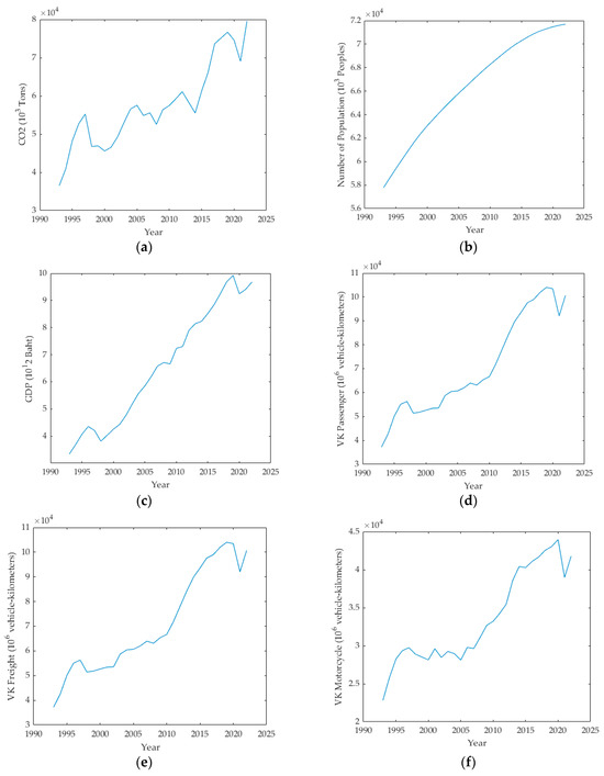
Figure 6. Historical trends of (a) emissions; (b) population; (c) GDP; (d) VK—passenger; (e) VK—freight; and (f) VK—motorcycle.

During the data preprocessing phase, a thorough search for missing data was conducted across all variables, and it was determined that no missing data points were present. Subsequently, outlier detection was performed utilizing the Z-score method. For each variable, Z-scores were calculated; any data points exceeding the threshold of ±3 were considered potential outliers. The analysis revealed that no outliers were detected within the dataset. These results indicate that the dataset is complete and devoid of extreme values, thereby making it suitable for subsequent analysis.

3.2. ANN Results

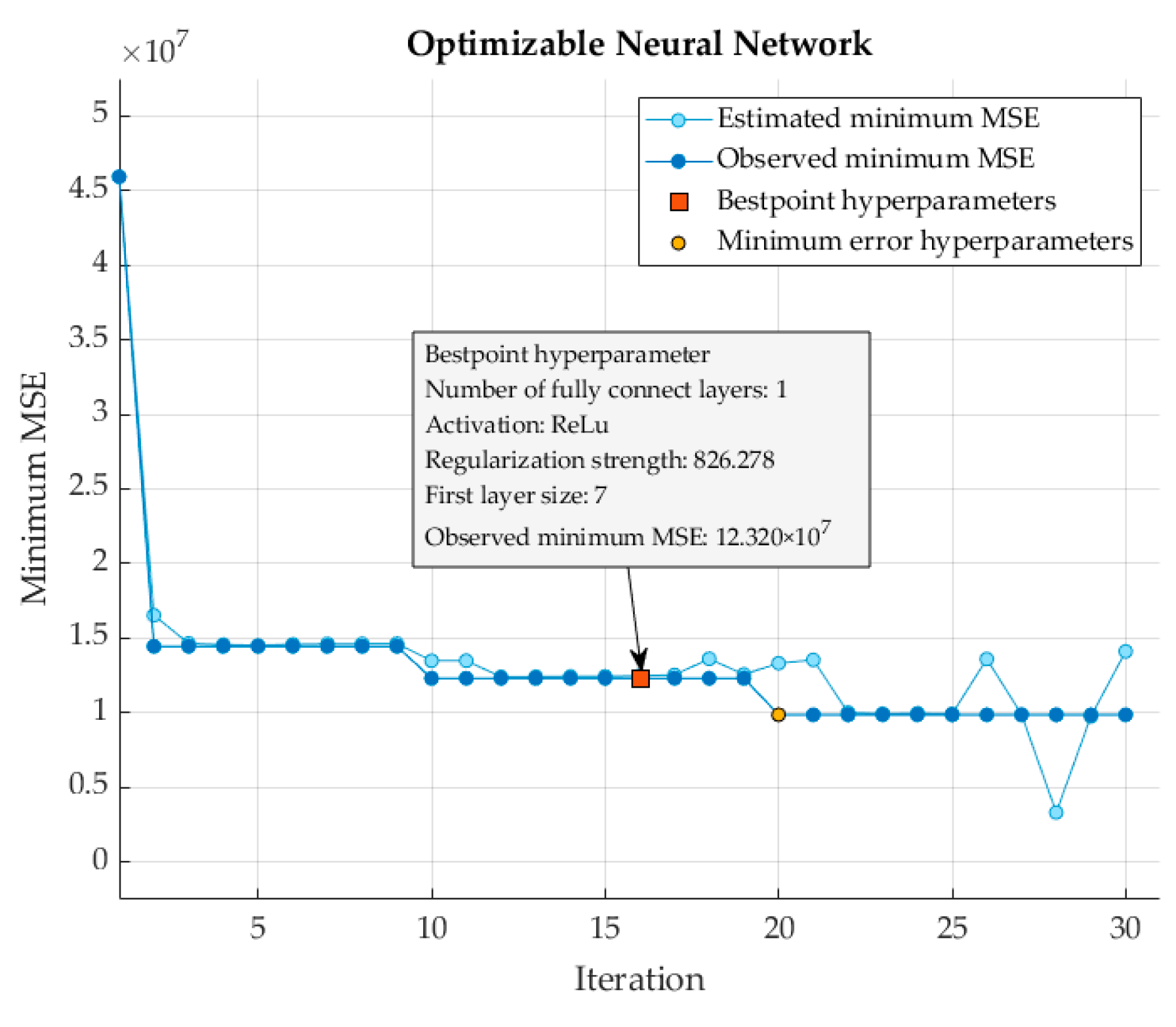
The selection of hyperparameters for the ANN model was driven by an optimization process using Bayesian optimization, which is designed to minimize the Mean Squared Error (MSE). The optimal model configuration included a single hidden layer with seven neurons. This size was chosen to balance complexity and generalizability, avoiding both underfitting and overfitting. The ReLU activation function was used for its efficiency and ability to introduce non-linearity, enhancing the model’s ability to learn complex patterns. A regularization coefficient of 826.227 was determined to be optimal, providing a penalty that helps prevent overfitting.

In this study, the structure of the ANN model underwent Bayesian optimization, using predefined hyperparameter search ranges, as outlined in Table 5. The optimization process yielded a minimum MSE value of 12.320 × 10⁷, accompanied by an RMSE of 3715.4. The optimized ANN architecture comprised a single, fully connected layer with a hidden layer size of seven neurons; employing the ReLU activation function and a regularization coefficient of 826.227. This configuration resulted in an enhanced predictive performance on the test set, with performance metrics such as MAPE, RMSE, and MAE yielding values of 6.395, 5054.005, and 4259.170, respectively.

Table 5. Parameter ranges for ANN optimization.

Hyperparameter	Search Range
Number of fully connected layers	1–3
First layer size	1–300
Second layer size	1–300
Third layer size	1–300
Activation function	ReLu, Tanh, Sigmoid, None
Regularization strength	4.7619 × 10−7–4761.9048

When performing hyperparameter tuning using Bayesian optimization, the algorithm selected the set of hyperparameter values that minimized the upper confidence interval of the MSE objective model, rather than the set that minimized the MSE. The optimization process depicted in Figure 7 highlighted the convergence toward the minimum observed and predicted MSE values across 30 iterations, with the 20th iteration representing the minimum-error hyperparameter; while the 16th iteration represents the best-point hyperparameter.

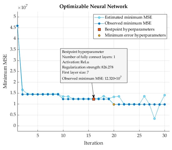
Figure 7. MSE optimization plot for the ANN.

3.3. SVR Results

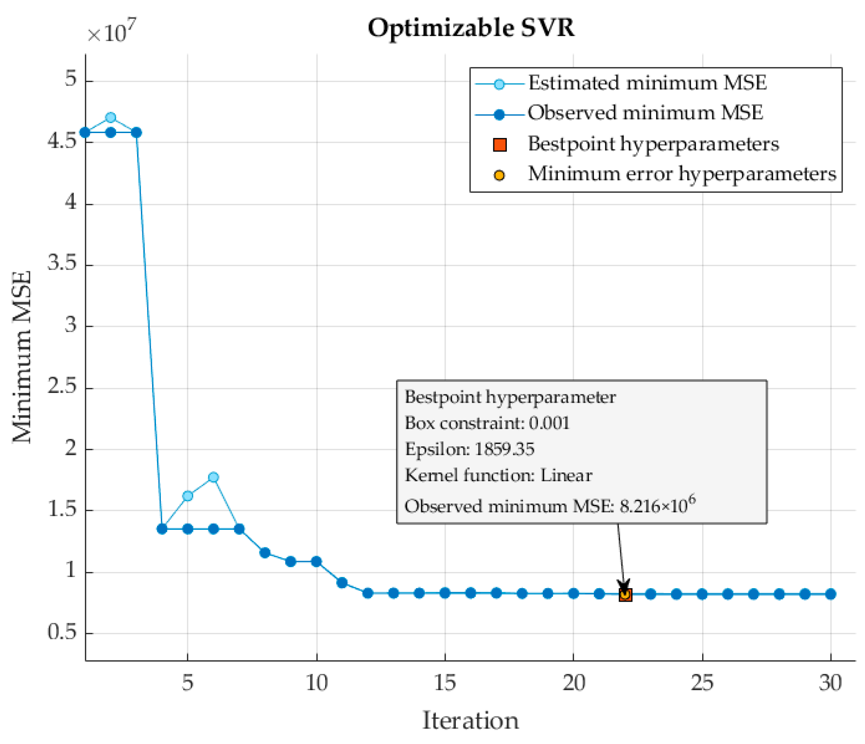
The hyperparameters for the SVR model were meticulously chosen to optimize model performance while balancing complexity and error tolerance. Specifically, a linear kernel, a box constraint (C) of 0.001, and an epsilon value of 1859.835 were chosen. A linear kernel simplifies a model and reduces computational complexity, making it ideal for assessing linear relationships between input features and the target variable. The small box constraint value of 0.001 imposes strong regularization, preventing overfitting by allowing some errors in the training data; thus maintaining a balance between bias and variance. The large epsilon value of 1859.835 enhances the model’s robustness with respect to outliers and noise by ignoring minor deviations from true values.

Bayesian optimization played a crucial role in this hyperparameter selection process, providing guidance through predefined search ranges to achieve optimal values, as detailed in Table 6. This iterative refinement process effectively balanced the model’s complexity and the error of the training data while maintaining tolerance margins around the predicted values. Notably, Figure 8 depicts the 22nd iteration, corresponding to both the minimum-error hyperparameter and the best-point hyperparameter, representing the optimal configuration with the lowest observed error.

Table 6. Parameter ranges for SVR optimization.

Hyperparameter	Search Range
Box constraint (C)	0.001–1000
epsilon	7.3489–734,887.3239
Kernel function	Gaussian, linear, quadratic, cubic

Figure 8. MSE optimization plot for the SVR.

A rigorous evaluation via three-fold cross-validation resulted in a minimum MSE value of 8.216 × 10⁶ and an impressive RMSE of 2866.3. Further assessment on an independent dataset revealed compelling performance metrics, including MAPE, RMSE, and MAE values of 7.628%, 6193.925, and 4865.085, respectively.

3.4. ARIMAX Results

All the exogenous variables in the training set have VIF values over 10, indicating a high degree of multicollinearity. To address this issue, stepwise regression was employed for variable selection and to reduce multicollinearity. The VK—Freight variable was selected as the exogenous variable. Then, the Augmented Dickey–Fuller (ADF) test for stationarity was conducted on the data, as presented in Table 7, showing that the data were found to be stationary at the first difference.

Table 7. Augmented Dickey–Fuller test.

ADF Test	No Difference	First Difference
Null rejected	False	True
p-Value	0.9220	0.0031
Test statistic	1.0927	−3.2928
Critical value	−1.9524	−1.9531
Significance level	0.05	0.05

Null hypothesis: The time series contains a unit root, which means that the data are nonstationary.

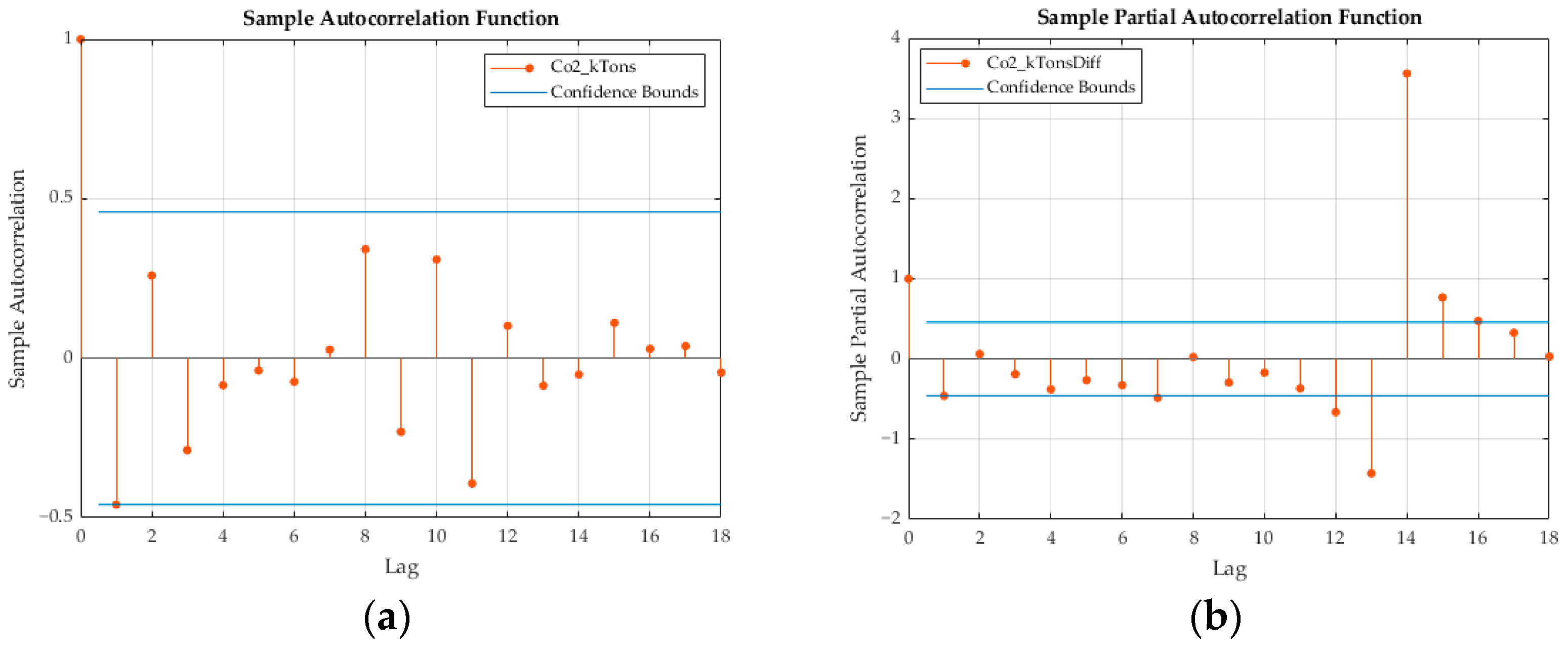
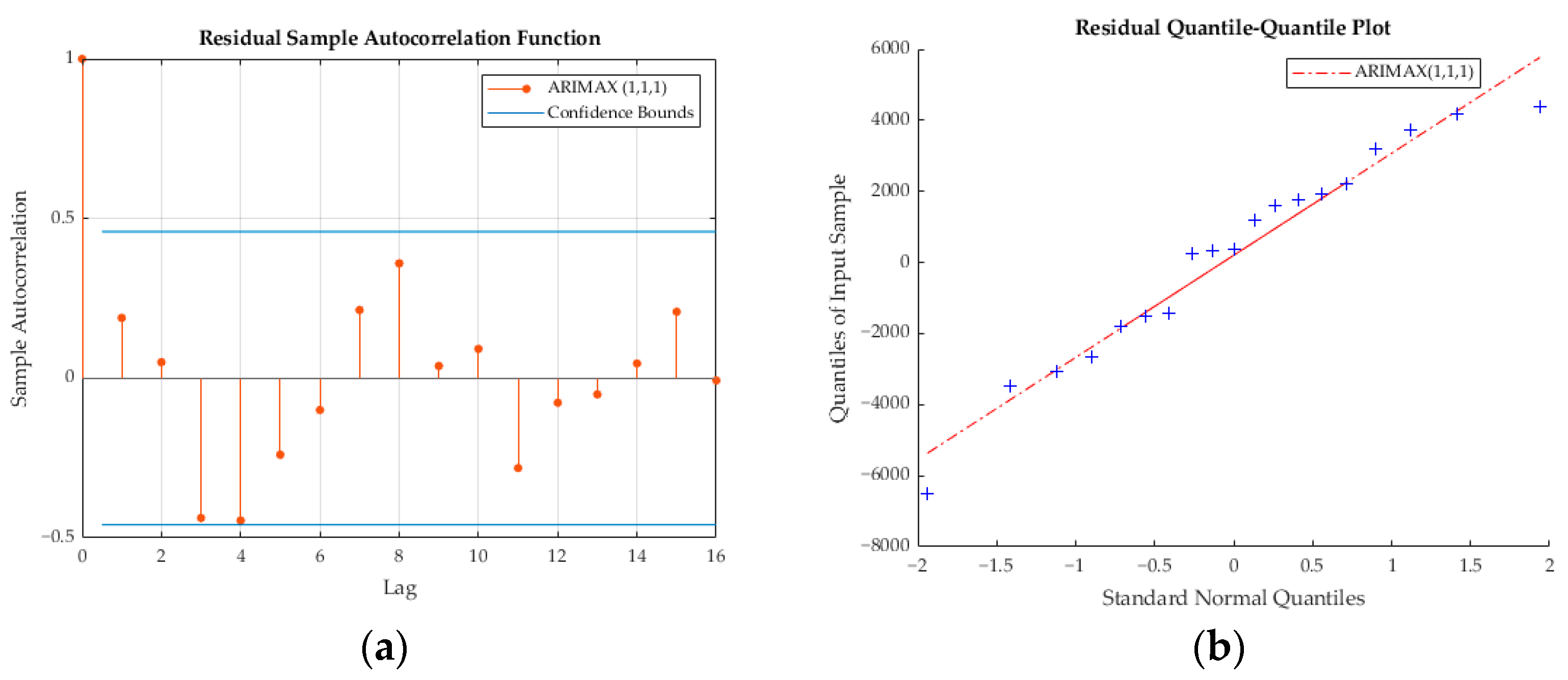
During the identification stage, a researcher visually examines the autocorrelation function (ACF) and partial autocorrelation function (PACF) plots of the differenced series in Figure 9. The PACF plot shows a significant spike at lag 1, which drops sharply afterward, indicating an autoregressive (AR) component at lag 1. The ACF plot also displays significant spikes at lag 1 that confirm the presence of an autoregressive component. Based on these observations, the suggested model was ARIMAX (1, 1, 1)—incorporating an AR (1) component and an MA (1) component—with a differencing of order 1 since the data are stationary at the first difference. The model also includes the exogenous variable “VK Freight”, which was selected after addressing multicollinearity through stepwise regression. Furthermore, in Figure 10, the autocorrelation function (ACF) plot demonstrates that most autocorrelations lie within the confidence bounds. This suggests that the residuals are essentially random and do not exhibit significant autocorrelation. It also implies that the model has effectively captured the time series data’s autocorrelation structure. Concurrently, the Quantile–Quantile (Q–Q) plot’s alignment with a straight line indicates that the residuals are normally distributed, thus affirming the assumption of normality, which is crucial for the validity of statistical inferences. Together, these diagnostic checks suggest that the model is reliable. Furthermore, the performance of the ARIMAX model was evaluated using several statistical measures; resulting in MAPE, RMSE, and MAE values of 9.286, 7916.483, and 6775.431, respectively. These figures serve as a testament to the model’s predictive accuracy and effectiveness when applied to our specific dataset.

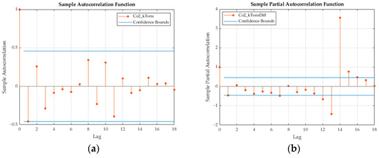
Figure 9. (a) ACF and (b) PACF plots of the differenced series.

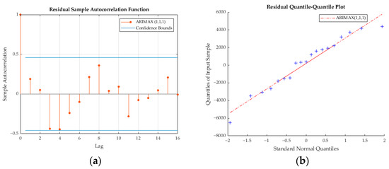
Figure 10. (a) ACF and (b) Q–Q plots of the ARIMAX (1, 1, 1) residuals.

3.5. HLN Test Results

The HLN test results in Table 8 provide evidence to reject the null hypothesis ($H_0$) of no difference in predictive accuracy between the compared models in all cases. For the comparison between ANN and SVR, the null hypothesis is rejected at the 5% significance level (HLN Statistic = 4.182 **), indicating a significant difference in predictive accuracy. Similarly, for the comparison between ANN and ARIMAX, the null hypothesis is rejected at the 1% significance level (HLN Statistic = 12.221 ***); this further demonstrates a significant difference. Additionally, the comparison between SVR and ARIMAX also leads to the rejection of the null hypothesis at the 5% significance level (HLN Statistic = 3.692 **). These results collectively indicate that the predictive accuracies of ANN, SVR, and ARIMAX models are significantly different from each other.

Table 8. HLN Test Results Comparing Predictive Accuracy of ANN, SVM, and ARIMAX Models.

Model	ANN	SVR	ARIMAX
ANN	—	4.182 **	12.221 ***
SVR	4.182 **	—	3.692 **
ARIMAX	12.221 ***	3.692 **	—

**, and *** denote significance at the 5%, and 1% levels, respectively.

4. Discussion

4.1. Model Performance

The performance of the ARIMAX model, although not subpar, may have been significantly influenced by its limitations—such as assuming stationarity and being sensitive to multicollinearity among predictors—and might not capture all the complexities of the analyzed data, such as external factors or sudden changes due to variants or policy changes. Given that this model’s forecasting was solely reliant on historical CO₂ emission and VK—freight data, with the test set corresponding to the year 2019, the ensuing global COVID-19 pandemic may have influenced the outcome. In particular, Thailand’s governmental lockdown measures led to a dramatic reduction in road traffic. This was primarily due to a shift in commuting behaviors for work, school, and other routine activities, as a growing number of individuals transitioned to remote work or online study. Furthermore, the transport and logistics sectors experienced considerable disruptions due to border closures and labor shortages. Collectively, these unforeseen circumstances constitute a significant event that has had a profound impact on CO₂ emissions within the transport sector.

Conversely, the ANN and SVR models exhibited superior and comparable results; as presented in Table 9 and Figure 11, respectively. The inherent adaptability of these models, as evidenced by their ability to consider a multitude of input variables, allowed them to better account for the widespread effects of the global COVID-19 pandemic. The ANN model, with its strength in capturing nonlinear relationships and its ability to learn from and generalize based on the input data, could model complex patterns and anomalies introduced by the pandemic. However, ANN models can sometimes act as black boxes, making it quite challenging to interpret the relationships between, and importance of, different input variables, and they may require larger datasets and more computational resources for training.

Table 9. Results regarding the performance evaluation metric.

Model	Evaluation Metric
	MAPE (%)	RSME (103 Tons)	MAE (103 Tons)
ANN	6.395	5054.005	4259.170
SVR	7.628	6193.925	4865.085
ARIMAX	9.286%	7916.483	6775.431

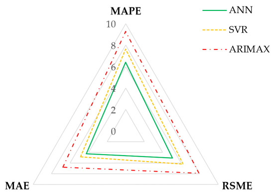
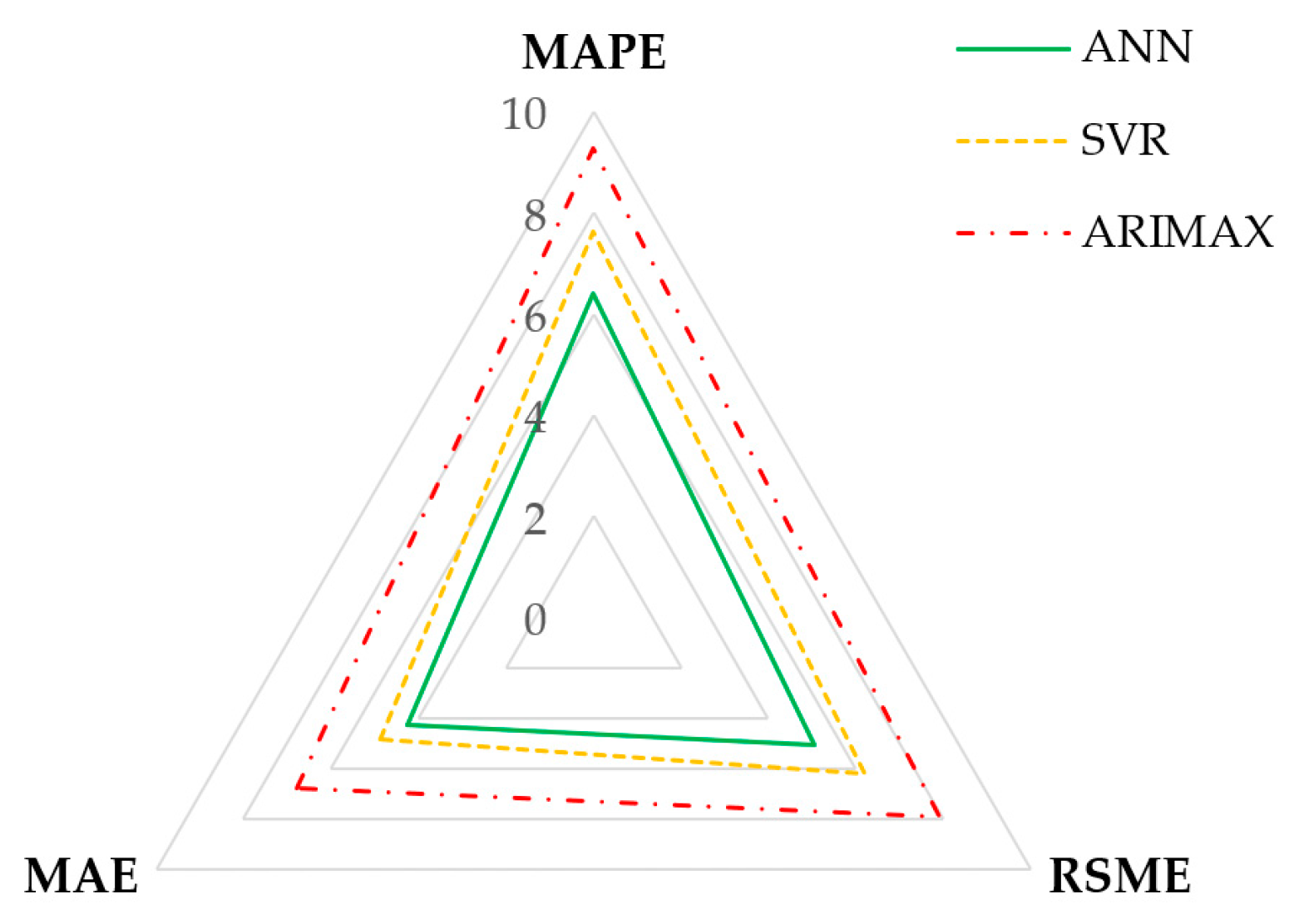
Figure 11. Radar graph of the performance evaluation metrics.

In comparison, SVR—with its foundation in statistical learning theory—provides a robust and accurate predictive model, especially in scenarios with smaller datasets and high-dimensional space. SVR models are also capable of managing non-linearities by employing different kernel functions. However, the selection of appropriate kernel functions and the tuning of parameters such as the box constraint and kernel coefficients can be computationally intensive and may require domain expertise to avoid overfitting or underfitting issues.

Therefore, the resilience demonstrated by the ANN and SVR models under these challenging conditions underscores their potential suitability for accurately predicting CO₂ emissions in the face of future unforeseeable events; albeit with considerations for their respective strengths and limitations in terms of model interpretability, parameter tuning, and computational requirements.

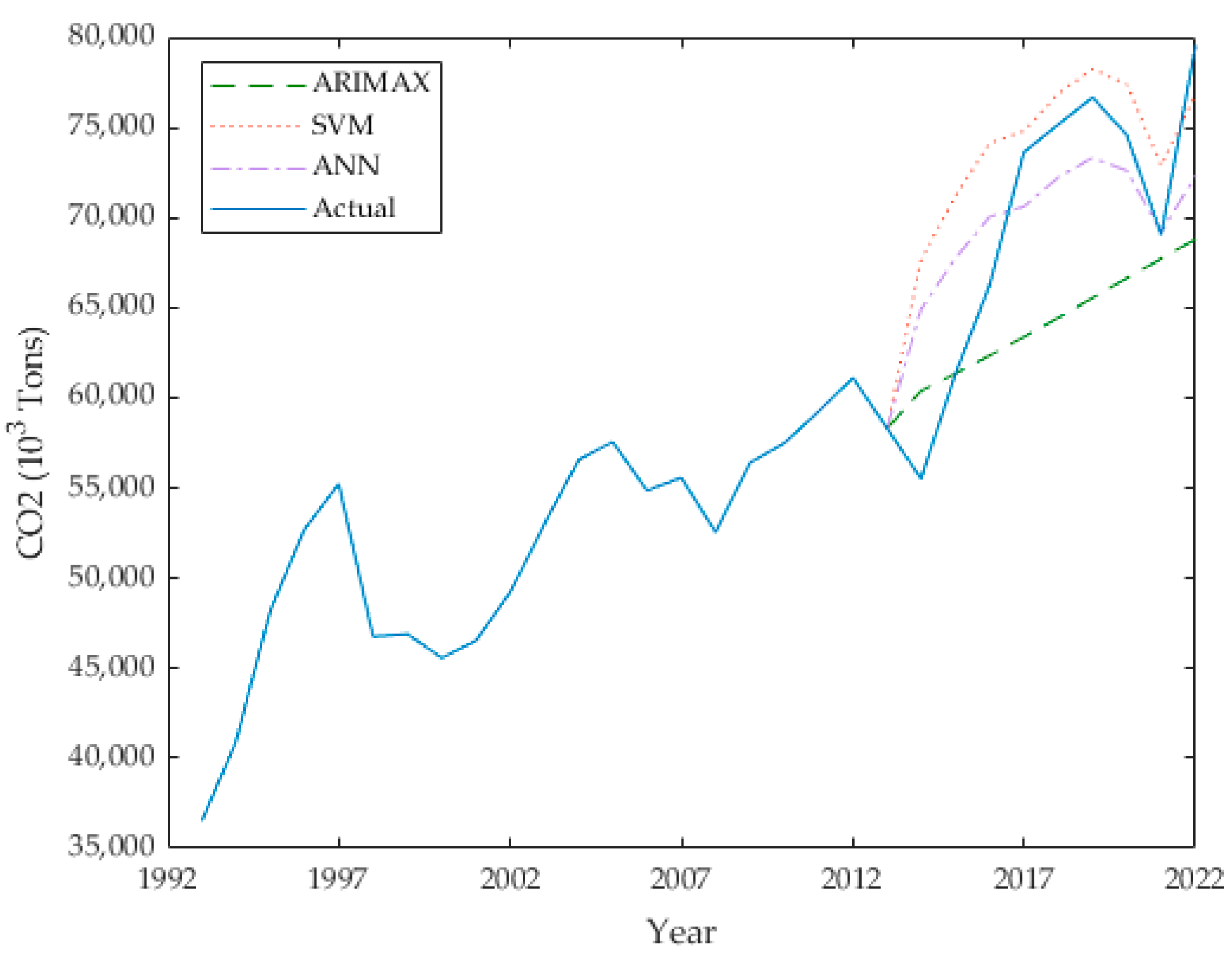
The HLN test results confirm significant differences in predictive accuracy among the compared models. Specifically, the null hypothesis of no difference in predictive accuracy is rejected for the comparisons between ANN and SVR (HLN Statistic = 4.182, **), ANN and ARIMAX (HLN Statistic = 12.221, ***); and SVR and ARIMAX (HLN Statistic = 3.692, **). This indicates that the predictive accuracies of ANN, SVR, and ARIMAX models are significantly different from each other. In terms of model evaluation, each algorithm demonstrated high accuracy in forecasting, as indicated by the metric MAPE in Table 4 and Table 9. For an overview, refer to Figure 11, which presents a radar graph that displays the results for each statistical metric. In this graph, the statistical metrics are scaled from 0 to 10, with RMSE and MAE specifically measured in units of million tons. The ANN model showed the lowest errors across all the metrics; with an MAE of 4.259, an RMSE of 5.054, and an MAPE of 6.395. This indicates superior performance in capturing the complex impacts of COVID-19 on CO₂ emissions. The SVR model, while slightly less accurate—with an MAE of 4.865, an RMSE of 6.194, and an MAPE of 7.628—still performed significantly better than the ARIMAX model. The ARIMAX model had the highest errors—with an MAE of 6.775, an RMSE of 7.916, and an MAPE of 9.286—reflecting its limitations in adapting to the sudden changes induced by the pandemic. The forecasting performance on the test set for each model is illustrated in Figure 12.

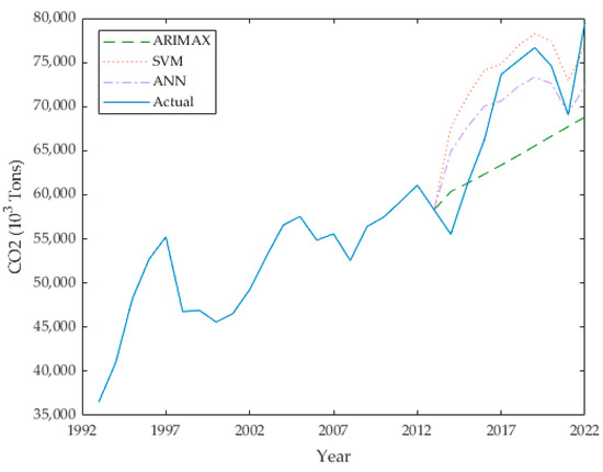
Figure 12. A comparison of the actual and predicted values for CO₂ emissions for each model for the test set.

4.2. Forecasting and Scenarios

Thailand’s “30@30” policy aspires to ensure that electric vehicles (EVs) constitute at least 30% of the nation’s total vehicle production by 2030. This policy prioritizes the promotion of EV usage across various transportation modes, including passenger vehicles, freight transport, and motorcycles. This initiative aims to transition energy consumption in the transportation sector to green energy sources, thereby enhancing energy efficiency and reducing greenhouse gas (GHG) emissions. Researchers have hypothesized that, pursuant to this policy, 30% of vehicle-kilometers will correspond to electric vehicles by 2030. The scenario analysis conducted based on this policy compares the expected impact of the “30@30” policy against a benchmark scenario without the policy influence. The aim is to evaluate the potential reduction in CO₂ emissions if the policy is implemented successfully. To evaluate the potential impact of the “30@30” policy, a comparison of two scenarios was conducted, specifically for the year 2030.

• The Benchmark Scenario: This scenario assumes the continuation of current vehicle usage patterns and reliance on traditional energy sources.
• The Policy Scenario: This scenario incorporates the effects of the “30@30” policy, hypothesizing that 30% of vehicle-kilometers will shift to electric vehicles by 2030. The independent variables VK—passenger, VK—freight, and VK—motorcycle are adjusted to reflect this shift, while GDP and population remain the same as they are in the benchmark scenario.

In prior research, datasets spanning 24 years were employed to predict outcomes over a 15-year span [17]; 15-years-ahead forecasts, as in this study, aligned with the LT-LEDS and Thailand’s National Strategy for the years 2023 to 2037 [5]. A 15-year forecast (from 2023 to 2037) was made to assess the long-term trends in CO₂ emissions under the benchmark scenario.

An ANN model was employed to forecast CO₂ emissions, using independent variables predicted from available data via the ARIMA model. The dataset was partitioned, with 70% designated to be used for model training, while the remaining 30% was utilized for performance evaluation using MAPE. The utilized models are shown in Table 10. For the population variable the model was specified as the ARIMA (0,2,1); this achieved a MAPE of 0.376%, indicating very precise predictions. The models for GDP, VK—Passenger, VK—Freight, and VK—Motorcycle were specified as ARIMA (0,1,0), indicating that these series follow a random walk [64,65]. A random walk is a stochastic process formed by the cumulative summation of independent, identically distributed random variables [66]. In these models, future values of the series cannot be predicted from past values, except through differencing; with each value resulting from the previous value plus a random shock. These series do not exhibit significant lagged relationships or moving average processes beyond what is captured through differencing, emphasizing their random walk characteristics. The results in Table 10 demonstrate acceptable MAPE values for all models, as previously mentioned. These results indicate the suitability of these models for forecasting independent variables in future CO₂ predictions.

Table 10. Assessment of the accuracy of the ARIMA models in forecasting independent variables.

Variable	ARIMA Model (p,d,q)	MAPE (%)
Population	(0,2,1)	0.376
GDP	(0,1,0)	3.165
VK—passenger	(0,1,0)	6.024
VK—freight	(0,1,0)	5.692
VK—motorcycle	(0,1,0)	3.210

Table 11 illustrates an increasing trend in CO₂ emissions, reflecting the continuation of current vehicle usage patterns and reliance on traditional energy sources. The results of the 15-year forecast indicate that, without intervention, CO₂ emissions will continue to rise, reaching 82,880.635 kTons by 2037. By 2030, the Benchmark Scenario predicts that emissions will reach 78,514.470 kTons. In contrast, the Policy Scenario, influenced by the “30@30” policy, forecasts a reduction in emissions to 63,517.583 kTons. The scenario analysis comparing these two scenarios reveals a substantial decrease in CO₂ emissions from fuel combustion in the transportation sector. This reduction underscores this policy’s effectiveness in mitigating emissions through enhancing energy efficiency and the increased utilization of renewable energy sources. Importantly, the anticipated transition to electric vehicles substantially contributes to the reduction in emissions from fuel combustion, highlighting this policy’s potential in fostering environmental sustainability.

Table 11. Future forecast of transportation-based CO₂ emissions in Thailand.

Year	Prediction (103 Tons)
2027	76,339.847
2032	79,864.493
2037	82,880.635

5. Conclusions

This study, in which we utilized ML data from 1993 to 2022 and employed models such as SVR and an ANN, demonstrated superior forecasting performance when compared to the traditional ARIMAX model. These ML models incorporate additional inputs, thereby exhibiting a reduced impact from the COVID-19 pandemic compared with that for ARIMAX, which relied on historical CO₂ emission and VK—freight data. Nevertheless, all three models displayed high predictive accuracy, as evidenced by the MAPE being less than or equal to 10% [8,56,57]. Upon consideration of performance metrics such as RMSE, MAE, and MAPE, the ANN model emerged as the most fitting choice for forecasting CO₂ emissions in Thailand. However, while this study primarily delved into Thailand’s transportation-related carbon emissions, its methodologies and findings can be adapted for application to other countries facing similar challenges pertaining to transportation-related CO₂ emissions. By examining factors such as population growth, GDP, and vehicle-kilometers traveled, this study sheds light on the underlying dynamics shaping emissions trends. Other countries can replicate this approach by conducting similar analyses that are tailored to their specific contexts. Furthermore, while the specific results may vary depending on factors such as data availability and quality, the overarching methodology can be adapted and applied by other countries seeking to improve their own emission forecasting capabilities. The scenario analysis demonstrated that Thailand’s “30@30” policy has the potential to make a significant impact on reduction of CO₂ emissions from fuel combustion in the transportation sector by encouraging the widespread adoption of electric vehicles and improving energy efficiency. By comparing the Policy Scenario with the Benchmark Scenario, the analysis predicted a substantial decrease in CO₂ emissions, underscoring this policy’s effectiveness. This policy not only promotes environmental sustainability by reducing greenhouse gas emissions but also stimulates economic growth and technological advancements, underscoring the crucial role of policy measures in advancing both environmental and economic sustainability.

6. Limitations and Future Research

Our study is not without its limitations. In particular, the relatively small dataset, combined with the significant impact of the COVID-19 pandemic, introduced a degree of uncertainty into our results. Thus, future research should focus on the potential impact of electric vehicles on CO₂ emissions, thereby contributing to a more comprehensive understanding of the role of sustainable technologies in reducing Thailand’s overall carbon footprint.

References

- EPA. Overview of Greenhouse Gases. Available online: https://www.epa.gov/ghgemissions/overview-greenhouse-gases (accessed on 21 December 2023).
- NOAA. Increase in Atmospheric Methane Set Another Record during 2021. Available online: https://www.noaa.gov/news-release/increase-in-atmospheric-methane-set-another-record-during-2021 (accessed on 21 December 2023).
- Bolan, S.; Padhye, L.P.; Jasemizad, T.; Govarthanan, M.; Karmegam, N.; Wijesekara, H.; Amarasiri, D.; Hou, D.; Zhou, P.; Biswal, B.K.; et al. Impacts of climate change on the fate of contaminants through extreme weather events. Sci. Total Environ. 2024, 909, 168388. [Google Scholar] [CrossRef] [PubMed]
- IPCC. Global Warming of 1.5 °C: Summary for Policymakers. Available online: https://www.ipcc.ch/sr15/chapter/spm/ (accessed on 21 December 2023).
- ONEP. Thailand’s Nationally Determined Contribution Roadmap on Mitigation 2021–2030; Office of Natural Resources and Environmental Policy and Planning: Bangkok, Thailand, 2020. [Google Scholar]
- ONEP. Thailand’s Fourth Biennial Update Report (BUR4); Office of Natural Resources and Environmental Policy and Planning: Bangkok, Thailand, 2022. [Google Scholar]
- Rogelj, J.; Den Elzen, M.; Höhne, N.; Fransen, T.; Fekete, H.; Winkler, H.; Schaeffer, R.; Sha, F.; Riahi, K.; Meinshausen, M. Paris Agreement climate proposals need a boost to keep warming well below 2 C. Nature 2016, 534, 631–639. [Google Scholar] [CrossRef] [PubMed]
- Ağbulut, Ü. Forecasting of transportation-related energy demand and CO2 emissions in Turkey with different machine learning algorithms. Sustain. Prod. Consum. 2022, 29, 141–157. [Google Scholar] [CrossRef]
- Sahraei, M.A.; Duman, H.; Çodur, M.Y.; Eyduran, E. Prediction of transportation energy demand: Multivariate Adaptive Regression Splines. Energy 2021, 224, 120090. [Google Scholar] [CrossRef]
- Tawiah, K.; Daniyal, M.; Qureshi, M. Pakistan CO2 Emission Modelling and Forecasting: A Linear and Nonlinear Time Series Approach. J. Environ. Public Health 2023, 2023, 5903362. [Google Scholar] [CrossRef] [PubMed]
- Ning, L.; Pei, L.; Li, F. Forecast of China’s Carbon Emissions Based on ARIMA Method. Discret. Dyn. Nat. Soc. 2021, 2021, 1441942. [Google Scholar] [CrossRef]
- Xu, G.; Schwarz, P.; Yang, H. Determining China’s CO2 emissions peak with a dynamic nonlinear artificial neural network approach and scenario analysis. Energy Policy 2019, 128, 752–762. [Google Scholar] [CrossRef]
- Liu, B.; Fu, C.; Bielefield, A.; Liu, Y.Q. Forecasting of Chinese Primary Energy Consumption in 2021 with GRU Artificial Neural Network. Energies 2017, 10, 1453. [Google Scholar] [CrossRef]
- Sun, W.; Liu, M. Prediction and analysis of the three major industries and residential consumption CO2 emissions based on least squares support vector machine in China. J. Clean. Prod. 2016, 122, 144–153. [Google Scholar] [CrossRef]
- Nyoni, T.; Bonga, W.G. Prediction of CO2 Emissions in India using ARIMA Models. DRJ-J. Econ. Financ. 2019, 4, 01–10. [Google Scholar]
- Fatima, S.; Saad, S.; Zia, S.; Hussain, E.; Fraz, T.; Mehwish, S.; Khan. Forecasting Carbon Dioxide Emission of Asian Countries Using ARIMA and Simple Exponential Smoothing Models. Int. J. Econ. Environ. Geol. 2019, 10, 64–69. [Google Scholar] [CrossRef]
- Ratanavaraha, V.; Jomnonkwao, S. Trends in Thailand CO2 emissions in the transportation sector and Policy Mitigation. Transp. Policy 2015, 41, 136–146. [Google Scholar] [CrossRef]
- Sutthichaimethee, P.; Ariyasajjakorn, D. Forecast of Carbon Dioxide Emissions from Energy Consumption in Industry Sectors in Thailand. Environ. Clim. Technol. 2018, 22, 107–117. [Google Scholar] [CrossRef]
- Salangam, S. Towards a predictor for CO2 emission usingregression analysis and an artificial neural network. J. Ind. Technol. Suan SunandhaRajabhat Univ. 2022, 10, 54–65. [Google Scholar]
- Yun, S.; Zanetti, R. Bayesian Estimation with Artificial Neural Network. In Proceedings of the 2021 IEEE 24th International Conference on Information Fusion (FUSION), Sun City, South Africa, 1–4 November 2021; pp. 1–7. [Google Scholar]
- Guh, R.-S. Effects of Non-Normality on Artificial Neural Network Based Control Chart Pattern Recognizer. J. Chin. Inst. Ind. Eng. 2002, 19, 13–22. [Google Scholar] [CrossRef]
- Shen, S.; Du, Y.; Xu, Z.; Qin, X.; Chen, J. Temperature Prediction Based on STOA-SVR Rolling Adaptive Optimization Model. Sustainability 2023, 15, 11068. [Google Scholar] [CrossRef]
- Kongcharoen, C.; Kruangpradit, T. Autoregressive integrated moving average with explanatory variable (ARIMAX) model for Thailand export. In Proceedings of the 33rd International Symposium on Forecasting, Seoul, Republic of Korea, 23–26 June 2013; pp. 1–8. [Google Scholar]
- Ling, A.; Darmesah, G.; Chong, K.; Ho, C. Application of ARIMAX model to forecast weekly cocoa black pod disease incidence. Math. Stat. 2019, 7, 29–40. [Google Scholar]
- Peter, Ď.; Silvia, P. ARIMA vs. ARIMAX—Which approach is better to analyze and forecast macroeconomic time series. In Proceedings of the 30th International Conference Mathematical Methods in Economics, Karviná, Czech Republic, 11–13 September 2012; pp. 136–140. [Google Scholar]
- Ghalandari, M.; Forootan Fard, H.; Komeili Birjandi, A.; Mahariq, I. Energy-related carbon dioxide emission forecasting of four European countries by employing data-driven methods. J. Therm. Anal. Calorim. 2021, 144, 1999–2008. [Google Scholar] [CrossRef]
- Faruque, M.O.; Rabby, M.A.J.; Hossain, M.A.; Islam, M.R.; Rashid, M.M.U.; Muyeen, S.M. A comparative analysis to forecast carbon dioxide emissions. Energy Rep. 2022, 8, 8046–8060. [Google Scholar] [CrossRef]
- Shabri, A. Forecasting the annual carbon dioxide emissions of Malaysia using Lasso-GMDH neural network-based. In Proceedings of the 2022 IEEE 12th Symposium on Computer Applications & Industrial Electronics (ISCAIE), Virtual, 21–22 May 2022; pp. 123–127. [Google Scholar]
- Rahman, A.; Hasan, M.M. Modeling and forecasting of carbon dioxide emissions in Bangladesh using Autoregressive Integrated Moving Average (ARIMA) models. Open J. Stat. 2017, 7, 560–566. [Google Scholar] [CrossRef]
- Kour, M. Modelling and forecasting of carbon-dioxide emissions in South Africa by using ARIMA model. Int. J. Environ. Sci. Technol. 2023, 20, 11267–11274. [Google Scholar] [CrossRef]
- Kamoljitprapa, P.; Sookkhee, S. Forecasting models for carbon dioxide emissions in major economic sectors of Thailand. J. Phys. Conf. Ser. 2022, 2346, 012001. [Google Scholar] [CrossRef]
- Zhu, C.; Wang, M.; Du, W. Prediction on Peak Values of Carbon Dioxide Emissions from the Chinese Transportation Industry Based on the SVR Model and Scenario Analysis. J. Adv. Transp. 2020, 2020, 8848149. [Google Scholar] [CrossRef]
- Li, Y.; Wei, Y.; Dong, Z. Will China Achieve Its Ambitious Goal?—Forecasting the CO2 Emission Intensity of China towards 2030. Energies 2020, 13, 2924. [Google Scholar] [CrossRef]
- Yang, S.; Wang, Y.; Ao, W.; Bai, Y.; Li, C. Prediction and analysis of CO2 emission in Chongqing for the protection of environment and public health. Int. J. Environ. Res. Public Health 2018, 15, 530. [Google Scholar] [CrossRef] [PubMed]
- Chandola, V.; Banerjee, A.; Kumar, V. Anomaly detection: A survey. ACM Comput. Surv. (CSUR) 2009, 41, 1–58. [Google Scholar] [CrossRef]
- Wilcox, R.R. Applying Contemporary Statistical Techniques; Elsevier: Amsterdam, The Netherlands, 2003. [Google Scholar]
- Yaro, A.S.; Maly, F.; Prazak, P. Outlier Detection in Time-Series Receive Signal Strength Observation Using Z-Score Method with Sn Scale Estimator for Indoor Localization. Appl. Sci. 2023, 13, 3900. [Google Scholar] [CrossRef]
- Swinscow, T.D.V.; Campbell, M.J. Statistics at Square One; BMJ Publishing Group: London, UK, 2002. [Google Scholar]
- Zhang, Z.; Beck, M.W.; Winkler, D.A.; Huang, B.; Sibanda, W.; Goyal, H. Opening the black box of neural networks: Methods for interpreting neural network models in clinical applications. Ann. Transl. Med. 2018, 6, 216. [Google Scholar] [CrossRef] [PubMed]
- Junhuathon, N.; Chayakulkheeree, K. Deep-learning-based short-term photovoltaic power generation forecasting using improved self-organization map neural network. J. Renew. Sustain. Energy 2022, 14, 043702. [Google Scholar] [CrossRef]
- Drucker, H.; Burges, C.J.; Kaufman, L.; Smola, A.; Vapnik, V. Support vector regression machines. In Proceedings of the 9th International Conference on Neural Information Processing Systems, Denver, Colorado, 2–5 December 1996; pp. 155–161. [Google Scholar]
- Schölkopf, B.; Smola, A.J.; Williamson, R.C.; Bartlett, P.L. New support vector algorithms. Neural Comput. 2000, 12, 1207–1245. [Google Scholar] [CrossRef]
- Cortes, C.; Vapnik, V. Support-vector networks. Mach. Learn. 1995, 20, 273–297. [Google Scholar] [CrossRef]
- Kao, Y.-S.; Nawata, K.; Huang, C.-Y. Predicting Primary Energy Consumption Using Hybrid ARIMA and GA-SVR Based on EEMD Decomposition. Mathematics 2020, 8, 1722. [Google Scholar] [CrossRef]
- Sutthison, T.; Thepchim, S. Application of Empirical Mode Decomposition with Box—Jankins and Support Vector Regression for Time Series Forecasting. J. Sci. Technol. Ubon Ratchathani Univ. 2020, 22, 59–74. [Google Scholar]
- Cho, H.U.; Nam, Y.; Choi, E.J.; Choi, Y.J.; Kim, H.; Bae, S.; Moon, J.W. Comparative analysis of the optimized ANN, SVM, and tree ensemble models using Bayesian optimization for predicting GSHP COP. J. Build. Eng. 2021, 44, 103411. [Google Scholar] [CrossRef]
- Dabboor, M.; Atteia, G.; Meshoul, S.; Alayed, W. Deep Learning-Based Framework for Soil Moisture Content Retrieval of Bare Soil from Satellite Data. Remote Sens. 2023, 15, 1916. [Google Scholar] [CrossRef]
- Snoek, J.; Larochelle, H.; Adams, R.P. Practical bayesian optimization of machine learning algorithms. Adv. Neural Inf. Process. Syst. 2012, 25. [Google Scholar]
- Elgeldawi, E.; Sayed, A.; Galal, A.R.; Zaki, A.M. Hyperparameter tuning for machine learning algorithms used for arabic sentiment analysis. Informatics 2021, 8, 79. [Google Scholar] [CrossRef]
- Jariego Pérez, L.C.; Garrido Merchán, E.C. Towards Automatic Bayesian Optimization: A first step involving acquisition functions. In Proceedings of the Advances in Artificial Intelligence: 19th Conference of the Spanish Association for Artificial Intelligence, CAEPIA 2020/2021, Málaga, Spain, 22–24 September 2021; Proceedings 19. pp. 160–169. [Google Scholar]
- Box, G.E.; Jenkins, G.M.; Reinsel, G.C.; Ljung, G.M. Time Series Analysis: Forecasting and Control; John Wiley & Sons: Hoboken, NJ, USA, 2015. [Google Scholar]
- Pankratz, A. Forecasting with Univariate Box-Jenkins Models: Concepts and Cases; John Wiley & Sons: Hoboken, NJ, USA, 2009. [Google Scholar]
- Chodakowska, E.; Nazarko, J.; Nazarko, Ł. ARIMA Models in Electrical Load Forecasting and Their Robustness to Noise. Energies 2021, 14, 7952. [Google Scholar] [CrossRef]
- Williams, B.M. Multivariate vehicular traffic flow prediction: Evaluation of ARIMAX modeling. Transp. Res. Rec. 2001, 1776, 194–200. [Google Scholar] [CrossRef]
- Kosow, H.; Gaßner, R. Methods of Future and Scenario Analysis: Overview, Assessment, and Selection Criteria; Deutsches Institut für Entwicklungspolitik: Bonn, Germany, 2007; Volume 39. [Google Scholar]
- Bakay, M.S.; Ağbulut, Ü. Electricity production based forecasting of greenhouse gas emissions in Turkey with deep learning, support vector machine and artificial neural network algorithms. J. Clean. Prod. 2021, 285, 125324. [Google Scholar] [CrossRef]
- Emang, D.; Shitan, M.; Abd Ghani, A.N.; Noor, K.M. Forecasting with univariate time series models: A case of export demand for peninsular Malaysia’s moulding and chipboard. J. Sustain. Dev. 2010, 3, 157. [Google Scholar] [CrossRef]
- Lewis, C. Industrial and Business Forecasting Methods; Butterworths: London, UK, 1982. [Google Scholar]
- Harvey, D.; Leybourne, S.; Newbold, P. Testing the equality of prediction mean squared errors. Int. J. Forecast. 1997, 13, 281–291. [Google Scholar] [CrossRef]
- Bianchi, D.; Büchner, M.; Tamoni, A. Bond risk premiums with machine learning. Rev. Financ. Stud. 2021, 34, 1046–1089. [Google Scholar] [CrossRef]
- Mizen, P.; Tsoukas, S. Forecasting US bond default ratings allowing for previous and initial state dependence in an ordered probit model. Int. J. Forecast. 2012, 28, 273–287. [Google Scholar] [CrossRef]
- Jiao, X.; Li, G.; Chen, J.L. Forecasting international tourism demand: A local spatiotemporal model. Ann. Tour. Res. 2020, 83, 102937. [Google Scholar] [CrossRef]
- Song, H.; Li, G.; Witt, S.F.; Athanasopoulos, G. Forecasting tourist arrivals using time-varying parameter structural time series models. Int. J. Forecast. 2011, 27, 855–869. [Google Scholar] [CrossRef]
- Nau, R. Introduction to ARIMA: Nonseasonal Models. Available online: https://people.duke.edu/~rnau/411arim.htm (accessed on 13 June 2024).
- Rhanoui, M.; Yousfi, S.; Mikram, M.; Merizak, H. Forecasting financial budget time series: ARIMA random walk vs LSTM neural network. IAES Int. J. Artif. Intell. 2019, 8, 317. [Google Scholar] [CrossRef]
- Lawler, G.F.; Limic, V. Random Walk: A Modern Introduction; Cambridge University Press: Cambridge, UK, 2010; Volume 123. [Google Scholar]
Disclaimer/Publisher’s Note: The statements, opinions and data contained in all publications are solely those of the individual author(s) and contributor(s) and not of MDPI and/or the editor(s). MDPI and/or the editor(s) disclaim responsibility for any injury to people or property resulting from any ideas, methods, instructions or products referred to in the content. |
© 2024 by the authors. Licensee MDPI, Basel, Switzerland. This article is an open access article distributed under the terms and conditions of the Creative Commons Attribution (CC BY) license (https://creativecommons.org/licenses/by/4.0/).