Bayesian Prediction of Order Statistics Based on k-Record Values from a Generalized Exponential Distribution

Abstract

We examine in this paper the implementation of Bayesian point predictors of order statistics from a future sample based on the $k^{\mathrm{th}}$ lower record values from a generalized exponential distribution.

1. Introduction

Let $\{X_n,n\ge 1\}$ be a sequence of independent and identically distributed (iid) random variables with a cumulative distribution function (cdf) $F(x;\theta )$ and a probability density function (pdf) $f(x;\theta )$, where $\theta \in \mathsf{\Theta }$ could be a real-valued vector. We will say that $X_j$ is an upper (lower) record value if it exceeds all previous random variables, i.e., if $X_j>(<)X_i$ for all $j>i$. By definition, $X_1$ is the first upper and lower record value.

The origin of the record value theory goes back to [1], where record values were introduced as a model of the successive extreme sequence of iid random variables. Record value theory for the iid case has been studied quite extensively in the literature. See, e.g., [2,3] for a detailed survey and the references inside.

In the continuous case, the definition of the $k^{\mathrm{th}}$ record values is as follows: For a fixed k, we define the sequence $\{T_{n,k},n\ge 1\}$, of the $k^{\mathrm{th}}$ lower record times of $\{X_n,n\ge 1\}$ as follows:

$$\begin{array}{cc}\hfill T_{1,k}& =1,\hfill \\ \hfill T_{n+1,k}& =min\{j>T_{n,k}:X_{k:T_{n,k}+k-1}>X_{k:j+k-1}\},n\ge 1,\hfill \end{array}$$

where $X_{j:n}$ denotes the $j^{\mathrm{th}}$ order statistic of the sample $(X_1,X_2,\dots ,X_n)$. The sequence $\{R_{n\left(k\right)},n\ge 1\}=\{X_{k:T_{n,k}+k-1},n\ge 1\}$ is called the sequence of the $k^{\mathrm{th}}$ lower record values of $\{X_n,n\ge 1\}$. In [2], these records are denoted as the Type 2 $k^{\mathrm{th}}$-record sequence. Note that for $k=1$, ordinary lower record times and values are recovered.

Record values can be found in many events in our everyday lives. We are especially interested in observing new records in meteorology, hydrology, sports, and so on. Their usefulness is found for characterization purposes, entropy measures, goodness-of-fit procedures, and various other statistical inferences.

The joint density function of the first n $k^{\mathrm{th}}$ lower records is obtained as (see [2]):

$$\begin{array}{c}\hfill f_{1,\dots ,n}(r_{1\left(k\right)},\dots ,r_{n\left(k\right)};\theta )=k^n{\left(F(r_{n\left(k\right)};\theta )\right)}^k\prod _{i=1}^n\frac{f(r_{i\left(k\right)};\theta )}{F(r_{i\left(k\right)};\theta )},r_{n\left(k\right)}<\dots <r_{1\left(k\right)},\end{array}$$

(1)

where ${\mathbf{r}}_{\left(\mathbf{k}\right)}=(r_{1\left(k\right)},\dots ,r_{n\left(k\right)})$ is denoted as an observed realization of ${\mathbf{R}}_{\left(\mathbf{k}\right)}=(R_{1\left(k\right)},\dots ,R_{n\left(k\right)})$.

Suppose that $Y_1,Y_2,\cdots ,Y_m$ are iid observations with cdf $F(x;\theta )$ and pdf $f(x;\theta )$, which are independent of the X-model. The order statistics of the sample are defined by the increasing order of $Y_1,Y_2,\cdots ,Y_m$, denoted as $Y_{1:m}\le Y_{2:m}\le \dots \le Y_{m:m}$. Order statistics have a broad use in statistics; their usefulness arises for characterization purposes, robust estimation, goodness-of-fit tests, reliability theory, quality control, and so on. Various literature works on order statistics can be found; for a detailed analysis, we recommend [4,5] and the references therein.

Prediction of future events based on current knowledge is a huge issue in statistics. It can be expressed in various contexts, and it can be generated in different forms. Several papers have been published on predicting future record values based on current records (see [2,3,6]) and prediction of future order statistics based on current order statistics (see [4,5,7]). The problem of predicting record values and order statistics from two independent sequences following two parameter exponential distributions was extensively discussed in [8].

The motivation behind this research follows from the point predictors of order statistics of a future sample from an exponential distribution based on the upper $k^{\mathrm{th}}$ record values published in [9]. In this paper, we deal with point predictors of order statistics based on the lower $k^{\mathrm{th}}$ record values from the generalized exponential distribution. Using a monotone transformation between the generalized exponential distribution and exponential distribution, we extend the associated inference and methodology found in [9] to our problem of interest.

This paper is organized as follows: In Section 2, we present a formal structure of the prior model distribution with related posterior densities of the $j^{\mathrm{th}}$ order statistics. The construction of predictive intervals and the expressions for point predictors of the order statistics from a future sample, with the maximum as a special case, is addressed in Section 3 and Section 4. The overall analysis of derived estimators is illustrated on a real data example and presented in Section 5.

2. Prior Information and Predictive Distributions

In general, the two parameter generalized exponential distribution with the shape parameter $\theta$ and scale parameter $\lambda$, denoted as $GED(\theta ,\lambda )$, is determined by the pdf and cdf of the form:

$$\begin{array}{cc}\hfill f(x;\theta ,\lambda )& =\theta \lambda e^{-\lambda x}{(1-e^{-\lambda x})}^{\theta -1},x>0,\hfill \end{array}$$

(2)

$$\begin{array}{cc}\hfill F(x;\theta ,\lambda )& ={(1-e^{-\lambda x})}^{\theta },x>0,\hfill \end{array}$$

(3)

where $\theta ,\lambda >0$.

In this work, we deal with the one-parameter generalized exponential distribution, denoted as GED($\theta$), with pdf and cdf given, respectively, by:

$$\begin{array}{cc}\hfill f(x;\theta )& =\theta e^{-x}{(1-e^{-x})}^{\theta -1},x>0,\hfill \end{array}$$

(4)

$$\begin{array}{cc}\hfill F(x;\theta )& ={(1-e^{-x})}^{\theta },x>0,\hfill \end{array}$$

(5)

where $\theta >0$ is a shape parameter.

The generalized exponential distribution (GED) is often recognized as a good alternative in situations when the Gamma and Weibull distributions lack efficient fits for skew data. For a detailed discussion about the GED, we refer to [10]. One of the several properties of this distribution family is that its nature (concave density, simple form of the pdf and cdf, behavior of the hazard rate function, simple procedure for generating random numbers) leads to easier modeling of skew data (see [11,12]). Specifically, we note that the GED distribution is a generalization of the standard exponential distribution (which can be obtained for $\theta =1$). The connection between $Exp\left(\theta \right)$ and $GED\left(\theta \right)$ is established by a monotone transformation $\tau (·)=-log(1-e^{-(·)})$. Several papers deal with estimation procedures for the parameters of the GE distribution based on records and order statistics (see, for example, Raqab and Ahsanullah [13]) and prediction inference for order statistics from the GED (see [7]).

Let us suppose we observed the first n $k^{\mathrm{th}}$ lower record values $R_{1\left(k\right)}=r_{1\left(k\right)},R_{2\left(k\right)}=r_{2\left(k\right)},...,R_{n\left(k\right)}=r_{n\left(k\right)}$ from GED($\theta$). From (4), (5), and (1), we can easily construct the likelihood function for $\theta$, given ${\mathbf{r}}_{\left(\mathbf{k}\right)}$, as:

$$\begin{array}{c}\hfill L\left(\theta \right|{\mathbf{r}}_{\left(\mathbf{k}\right)})=k^n{\theta }^{n}u\left({\mathbf{r}}_{\left(\mathbf{k}\right)}\right)e^{-\theta k\tau \left(r_{n\left(k\right)}\right)},r_{1\left(k\right)}>r_{2\left(k\right)}>...>r_{n\left(k\right)}>0,\end{array}$$

(6)

where $u\left({\mathbf{r}}_{\left(\mathbf{k}\right)}\right)={\prod }_{i=1}^n{e}^{-r_{i\left(k\right)}}/(1-e^{-r_{i\left(k\right)}})$ and $\tau \left(r_{n\left(k\right)}\right)=-log(1-e^{-r_{n\left(k\right)}})$. Here, we denote log as the natural logarithm.

Further, we can extend the reasoning about the parameter $\theta$ by supposing that it is a realization of a random variable with prior distribution:

$${\pi }_{(a,b)}\left(\theta \right)\propto {\theta }^{a-1}{e}^{-b\theta },\theta >0,$$

(7)

where $a,b>0$ are parameters of the prior distribution. These parameters are chosen in most cases based on realizations of previous experiments or relying on the knowledge that the researcher owns. With this in mind, it is easy to obtain the posterior distribution of $\theta$, given ${\mathbf{r}}_{\left(\mathbf{k}\right)}$, as:

$${\pi }_{(a,b)}\left(\theta \right|{\mathbf{r}}_{\left(\mathbf{k}\right)})=\frac{{(b+k\tau \left(r_{n\left(k\right)}\right))}^{n+a}}{\mathsf{\Gamma }(n+a)}{\theta }^{n+a-1}{e}^{-\theta (b+k\tau \left(r_{n\left(k\right)}\right))},\theta >0,$$

(8)

where $\mathsf{\Gamma }(·)$ is the complete gamma function. It is well known (see [14]) that the Bayes estimator of $\theta$, with respect to squared error loss (SEL), is the mean of the posterior density (8), i.e.,

$$\widehat{\theta }=\frac{n+a}{b+k\tau \left(r_{n\left(k\right)}\right)}.$$

(9)

The marginal density function of the $j^{\mathrm{th}}$ order statistic from a sample of size m from GED$\left(\theta \right)$ is given by (see [15]):

$$\begin{array}{c}\hfill f_{Y_{j:m}}\left(y\right|\theta )=\frac{1}{B(j;m-j+1)}\theta e^{-y}{(1-e^{-y})}^{\theta j-1}{(1-{(1-e^{-y})}^{\theta })}^{m-j},y>0,\end{array}$$

(10)

where $B(·;·)$ is the complete beta function.

The Bayesian predictive density of X, given ${\mathbf{r}}_{\left(\mathbf{k}\right)}$, is obtained as an integral of the posterior density (8) multiplied by the density function (4) with respect to $\theta$, i.e.,

$$\begin{array}{cc}{f}_{X|{\mathbf{r}}_{\left(\mathbf{k}\right)}}\left(x\right|{\mathbf{r}}_{\left(\mathbf{k}\right)})\hfill & ={\int }_{\theta }{f}_X\left(x\right|\theta ){\pi }_{(a,b)}\left(\theta \right|{\mathbf{r}}_{\left(\mathbf{k}\right)})d\theta \hfill \\ & =\frac{{(b+k\tau \left(r_{n\left(k\right)}\right))}^{n+a}}{\mathsf{\Gamma }(n+a)}\frac{e^{-x}}{1-e^{-x}}{\int }_0^{\infty }{\theta }^{n+a}{e}^{-\theta (b+k\tau \left(r_{n\left(k\right)}\right)+\tau \left(x\right))}d\theta \hfill \\ & =\frac{e^{-x}}{1-e^{-x}}\frac{n+a}{b+k\tau \left(r_{n\left(k\right)}\right)}{\left(1+\frac{\tau \left(x\right)}{b+k\tau \left(r_{n\left(k\right)}\right)}\right)}^{-n-a-1},x>0.\hfill \end{array}$$

(11)

By proceeding as before, the Bayesian predictive density of $Y_{j:m}$, given ${\mathbf{r}}_{\left(\mathbf{k}\right)}$, is obtained as an integral of the posterior density (8) multiplied by the conditional density (10) with respect to $\theta$, i.e.,

$$\begin{array}{cc}{f}_{Y_{j:m}}\left(y\right|{\mathbf{r}}_{\left(\mathbf{k}\right)})\hfill & ={\int }_{\theta }{f}_{Y_{j:m}}\left(y\right|\theta ){\pi }_{(a,b)}\left(\theta \right|{\mathbf{r}}_{\left(\mathbf{k}\right)})d\theta \hfill \\ & =\frac{e^{-y}}{1-e^{-y}}\frac{{(b+k\tau \left(r_{n\left(k\right)}\right))}^{n+a}}{\mathsf{\Gamma }(n+a)B(j;m-j+1)}\hfill \\ & \times \sum _{l=0}^{m-j}\left(\genfrac{}{}{0pt}{}{m-j}{l}\right){(-1)}^{m-j-l}{\int }_0^{\infty }{\theta }^{n+a}{e}^{-\theta (b+k\tau \left(r_{n\left(k\right)}\right)+(m-l)\tau \left(y\right))}d\theta \hfill \\ & =\frac{e^{-y}}{1-e^{-y}}\frac{{(b+k\tau \left(r_{n\left(k\right)}\right))}^{n+a}(n+a)}{B(j;m-j+1)}\sum _{l=0}^{m-j}\left(\genfrac{}{}{0pt}{}{m-j}{l}\right)\hfill \\ & \times \frac{{(-1)}^{m-j-l}}{{(b+k\tau \left(r_{n\left(k\right)}\right)+(m-l)\tau \left(y\right))}^{n+a+1}}\hfill \\ & =\frac{e^{-y}}{1-e^{-y}}\frac{(n+a)}{(b+k\tau \left(r_{n\left(k\right)}\right))B(j;m-j+1)}\sum _{l=0}^{m-j}\left(\genfrac{}{}{0pt}{}{m-j}{l}\right){(-1)}^{m-j-l}\hfill \\ & \times {\left(1+\frac{(m-l)\tau \left(y\right)}{b+k\tau \left(r_{n\left(k\right)}\right)}\right)}^{-n-a-1},y>0.\hfill \end{array}$$

(12)

For special cases $j=1$ and $j=m$, the previous formulae reduce to:

$$\begin{array}{cc}\hfill f_{Y_{1:m}}\left(y\right|{\mathbf{r}}_{\left(\mathbf{k}\right)})& =\frac{e^{-y}}{1-e^{-y}}\frac{m(n+a)}{(b+k\tau \left(r_{n\left(k\right)}\right))}\sum _{l=0}^{m-1}\left(\genfrac{}{}{0pt}{}{m-1}{l}\right){(-1)}^{m-1-l}\hfill \\ & \times {\left(1+\frac{(m-l)\tau \left(y\right)}{b+k\tau \left(r_{n\left(k\right)}\right)}\right)}^{-n-a-1},y>0,\hfill \end{array}$$

and:

$$\begin{array}{cc}\hfill f_{Y_{m:m}}\left(y\right|{\mathbf{r}}_{\left(\mathbf{k}\right)})& =\frac{m{e}^{-y}}{1-e^{-y}}\frac{n+a}{b+k\tau \left(r_{n\left(k\right)}\right)}{\left(1+\frac{m\tau \left(y\right)}{b+k\tau \left(r_{n\left(k\right)}\right)}\right)}^{-n-a-1},y>0,\hfill \end{array}$$

which represent the predictive densities of the minimum and the maximum of a future sample of size m, given ${\mathbf{r}}_{\left(\mathbf{k}\right)}$.

3. Prediction Intervals of Order Statistics

In this section, we construct $100(1-\alpha )\%$ prediction intervals for $Y_{j:m}$, given ${\mathbf{r}}_{\left(\mathbf{k}\right)},1\le j\le m.$

For the Bayesian two-sided equi-tailed interval, we need to obtain the solutions of the following equations

$$F_{Y_{j:m}}\left(L\right|{\mathbf{r}}_{\left(\mathbf{k}\right)})=\frac{\alpha }{2},and{F}_{Y_{j:m}}\left(U\right|{\mathbf{r}}_{\left(\mathbf{k}\right)})=1-\frac{\alpha }{2},$$

(13)

where L and U are lower and upper interval bounds, respectively, with $F_{Y_{j:m}}\left(x\right|{\mathbf{r}}_{\left(\mathbf{k}\right)})=P\{Y_{j:m}\le x|{\mathbf{r}}_{\left(\mathbf{k}\right)}\}$ as the predictive distribution function of $Y_{j:m}$, given ${\mathbf{r}}_{\left(\mathbf{k}\right)}$. Its form is given by:

$$\begin{array}{cc}\hfill F_{Y_{j:m}}\left(y\right|{\mathbf{r}}_{\left(\mathbf{k}\right)})& =\frac{1}{B(j;m-j+1)}\sum _{l=0}^{m-j}\left(\genfrac{}{}{0pt}{}{m-j}{l}\right)\frac{{(-1)}^{m-j-l}}{m-l}{\left(1+\frac{(m-l)\tau \left(y\right)}{b+k\tau \left(r_{n\left(k\right)}\right)}\right)}^{-n-a},\hfill \end{array}$$

(14)

for $y>0$. Due to a rather complicated form of (14), we can only find the solutions of (13) numerically.

If (12) possesses a unimodal shape, the $100(1-\alpha )\%$ highest posterior density (HPD) interval for $Y_{j:m},$ given ${\mathbf{r}}_{\left(\mathbf{k}\right)}$, could be presented by the set:

$$\begin{array}{c}\hfill R\left({\pi }_{\alpha }\right)=\{y:f_{Y_{j:m}}\left(y\right|{\mathbf{r}}_{\left(\mathbf{k}\right)})\ge {\pi }_{\alpha }\},\end{array}$$

where ${\pi }_{\alpha }$ is the largest constant such that $P(Y_{j:m}\in R\left({\pi }_{\alpha }\right))\ge 1-\alpha$. The lower and upper bounds of the $100(1-\alpha )\%$ HPD interval for this case, denoted as $(u_{Y_{j:m};1},u_{Y_{j:m};2})$, are the solutions of the following optimization problem (see [16], Theorem 1).

$$\begin{array}{c}\underset{u_{Y_{j:m};1}<u_{Y_{j:m};2}}{min}(|f_{Y_{j:m}}\left(u_{Y_{j:m};2}\right|{\mathbf{r}}_{\left(\mathbf{k}\right)})-f_{Y_{j:m}}\left(u_{Y_{j:m};1}\right|{\mathbf{r}}_{\left(\mathbf{k}\right)})|\hfill \\ +|F_{Y_{j:m}}\left(u_{Y_{j:m};2}\right|{\mathbf{r}}_{\left(\mathbf{k}\right)})-F_{Y_{j:m}}\left(u_{Y_{j:m};1}\right|{\mathbf{r}}_{\left(\mathbf{k}\right)})-(1-\alpha )\left|\right).\hfill \end{array}$$

(15)

In Section 5, we present the construction of these posterior intervals on an example.

Case When $j=m$ (Maximum of the Future Sample)

Within this special case, (14) simplifies to:

$$\begin{array}{c}\hfill F_{Y_{m:m}}\left(z\right|{\mathbf{r}}_{\left(\mathbf{k}\right)})={\left(1+\frac{m\tau \left(z\right)}{b+k\tau \left(r_{n\left(k\right)}\right)}\right)}^{-n-a},z>0,\end{array}$$

(16)

so we can express the lower ${\alpha }^{\mathrm{th}}$ quantile ${\xi }_{Y_{m:m},\alpha }(a,b)$ of (16) explicitly as:

$$\begin{array}{cc}\hfill {\xi }_{Y_{m:m},\alpha }(a,b)& =-log\left(1-exp\left\{-\frac{b+k\tau \left(r_{n\left(k\right)}\right)}{m}\left(\frac{1}{\sqrt[n+a]{\alpha }}-1\right)\right\}\right)\hfill \end{array}$$

(17)

$$\begin{array}{c}=\tau \left(\frac{b+k\tau \left(r_{n\left(k\right)}\right)}{m}\left(\frac{1}{\sqrt[n+a]{\alpha }}-1\right)\right).\hfill \end{array}$$

(18)

Therefore, it is then reasonable to think of the interval $(0,{\xi }_{Y_{m:m},1-\alpha })$ as the upper one-sided $100(1-\alpha )\%$ Bayesian predictive interval for $Y_{m:m}$, given ${\mathbf{r}}_{\left(\mathbf{k}\right)}$.

Moreover, we can directly obtain the $100(1-\alpha )\%$ Bayesian two-sided equi-tailed prediction interval for the maximum of a future sample of size m by:

$$\left[\tau \left(\frac{b+k\tau \left(R_{n\left(k\right)}\right)}{m}\left(\frac{1}{\sqrt[n+a]{\alpha /2}}-1\right)\right),\tau \left(\frac{b+k\tau \left(R_{n\left(k\right)}\right)}{m}\left(\frac{1}{\sqrt[n+a]{1-\alpha /2}}-1\right)\right)\right].$$

(19)

The uni-modal shape of the pdf of $Y_{m:m}$, given ${\mathbf{r}}_{\left(\mathbf{k}\right)}$, can be confirmed based on (16). Therefore, the procedure (15) for obtaining HPD intervals holds.

4. Point Predictors of Order Statistics

In this section, we obtain Bayes point predictors for order statistics from a future sample of size m based on the observed $k^{\mathrm{th}}$ lower record values, with respect to the squared error loss (SEL) function, as:

$$\begin{array}{ccc}{\widehat{Y}}_{j:m}\hfill & =\frac{{(b+k\tau \left(R_{n\left(k\right)}\right))}^{n+a}}{\mathsf{\Gamma }(n+a)B(j;m-j+1)}{\int }_0^{\infty }{\int }_0^{\infty }y{\theta }^{n+a}{e}^{-\theta (b+k\tau \left(R_{n\left(k\right)}\right))}{e}^{-y}\hfill & \hfill \\ \hfill & \times {(1-e^{-y})}^{\theta j-1}{(1-{(1-e^{-y})}^{\theta })}^{m-j}dyd\theta \hfill & \hfill \\ \hfill & =\frac{{(b+k\tau \left(R_{n\left(k\right)}\right))}^{n+a}}{\mathsf{\Gamma }(n+a)B(j;m-j+1)}\sum _{l=0}^{m-j}\left(\genfrac{}{}{0pt}{}{m-j}{l}\right){(-1)}^{m-j-l}{\int }_0^{\infty }{\theta }^{n+a}{e}^{-\theta (b+k\tau \left(R_{n\left(k\right)}\right))}\hfill & \hfill \\ \hfill & \times {\int }_0^{\infty }y{e}^{-y}{(1-e^{-y})}^{\theta (m-l)-1}dyd\theta \hfill & \hfill \\ \hfill & =\frac{{(b+k\tau \left(R_{n\left(k\right)}\right))}^{n+a}}{\mathsf{\Gamma }(n+a)B(j;m-j+1)}\sum _{l=0}^{m-j}\left(\genfrac{}{}{0pt}{}{m-j}{l}\right){(-1)}^{m-j-l}{\int }_0^{\infty }{\theta }^{n+a}{e}^{-\theta (b+k\tau \left(R_{n\left(k\right)}\right))}\hfill & \hfill \\ \hfill & \times {\int }_0^1(-log(1-t))t^{\theta (m-l)-1}dtd\theta \hfill & \hfill \\ \hfill & =\frac{{(b+k\tau \left(R_{n\left(k\right)}\right))}^{n+a}}{\mathsf{\Gamma }(n+a)B(j;m-j+1)}\sum _{l=0}^{m-j}\left(\genfrac{}{}{0pt}{}{m-j}{l}\right)\frac{{(-1)}^{m-j-l}}{m-l}{\int }_0^{\infty }{\theta }^{n+a-1}{e}^{-\theta (b+k\tau \left(R_{n\left(k\right)}\right))}\hfill & \hfill \\ \hfill & \times \left(\psi \right(1+\theta (m-l))-\psi (1\left)\right)d\theta ,\hfill \end{array}$$

(20)

where we have ${\int }_0^1(-log(1-t))t^{\theta (m-l)-1}dt=(\psi (1+\theta (m-l))-\psi \left(1\right))/\left(\theta (m-l)\right)$, according to ([17], p. 543), and where $\psi \left(x\right)=\frac{dlog\mathsf{\Gamma }\left(x\right)}{dx}$.

Let us denote:

$$\begin{array}{cc}\hfill & A(m,j,n,a,b,k,R_{n\left(k\right)})=\hfill \\ \hfill & \frac{{(b+k\tau \left(R_{n\left(k\right)}\right))}^{n+a}}{\mathsf{\Gamma }(n+a)B(j;m-j+1)}\sum _{l=0}^{m-j}\left(\genfrac{}{}{0pt}{}{m-j}{l}\right)\frac{{(-1)}^{m-j-l}}{m-l}{\int }_0^{\infty }{\theta }^{n+a-1}{e}^{-\theta (b+k\tau \left(R_{n\left(k\right)}\right))}\hfill & \hfill \\ \hfill & \times \left(\psi \right(1+\theta (m-l))-\psi (1\left)\right)d\theta .\hfill \end{array}$$

(21)

For special cases $j=1$ and $j=m$, we have:

$$\begin{array}{cc}\hfill {\widehat{Y}}_{1:m}& =\frac{m{(b+k\tau \left(R_{n\left(k\right)}\right))}^{n+a}}{\mathsf{\Gamma }(n+a)}\sum _{l=0}^{m-1}\left(\genfrac{}{}{0pt}{}{m-1}{l}\right)\frac{{(-1)}^{m-1-l}}{m-l}{\int }_0^{\infty }{\theta }^{n+a-1}{e}^{-\theta (b+k\tau \left(R_{n\left(k\right)}\right))}\hfill \\ & \times \left(\psi \right(1+\theta (m-l))-\psi (1\left)\right)d\theta \hfill \end{array}$$

and:

$$\begin{array}{cc}\hfill {\widehat{Y}}_{m:m}& =\frac{{(b+k\tau \left(R_{n\left(k\right)}\right))}^{n+a}}{\mathsf{\Gamma }(n+a)}{\int }_0^{\infty }{\theta }^{n+a-1}{e}^{-\theta (b+k\tau \left(R_{n\left(k\right)}\right))}(\psi (1+m\theta )-\psi \left(1\right))d\theta .\hfill \end{array}$$

Further, we find the mean squared prediction error (MSPE) of ${\widehat{Y}}_{j:m}$, for $1\le j\le m$, as:

$$\begin{array}{cc}MSPE\left({\widehat{Y}}_{j:m}\right)\hfill & =E{({\widehat{Y}}_{j:m}-Y_{j:m})}^2\hfill \\ & =E(A{(m,j,n,a,b,k,R_{n\left(k\right)})}^2-2A(m,j,n,a,b,k,R_{n\left(k\right)})Y_{j:m}+Y_{j:m}^2)\hfill \\ & =E{\left(A(m,j,n,a,b,k,R_{n\left(k\right)})\right)}^2-2E\left(A(m,j,n,a,b,k,R_{n\left(k\right)})\right)E\left(Y_{j:m}\right)\hfill \\ & +E\left(Y_{j:m}^2\right)\hfill \end{array}$$

(22)

The value of $MSPE\left({\widehat{Y}}_{j:m}\right)$ can only be estimated numerically because of its complicated form. For case $j=m$, the MSPE (22) slightly reduces its complexity.

Remark 1. When applying absolute error loss function, the point predictor of the maximum of a future sample is the median of the predictive density (12), i.e.,

$$\begin{array}{cc}\hfill {\widehat{Y}}_{m:m}& =\tau \left(\frac{b+k\tau \left(R_{n\left(k\right)}\right)}{m}\left(2^{\frac{1}{n+a}}-1\right)\right).\hfill \end{array}$$

Remark 1.

The flexibility of the shape of the prior density is allowed by considering mixtures of prior distributions. Following the same construction principle of (8), if we take $\pi \left(\theta \right)={\sum }_{j=1}^d{\beta }_j{\pi }_{(a_j,b_j)}\left(\theta \right)$ as a prior distribution, then $\pi \left(\theta \right|{\mathbf{r}}_{\left(\mathbf{k}\right)})={\sum }_{j=1}^d{\beta }_j\left({\mathbf{r}}_{\left(\mathbf{k}\right)}\right){\pi }_{(a_j,b_j)}\left(\theta \right|{\mathbf{r}}_{\left(\mathbf{k}\right)})$, where ${\beta }_s\left({\mathbf{r}}_{\left(\mathbf{k}\right)}\right)={\beta }_s{w}_s\left({\mathbf{r}}_{\left(\mathbf{k}\right)}\right)/{\sum }_{j=1}^d{\beta }_j{w}_j\left({\mathbf{r}}_{\left(\mathbf{k}\right)}\right)$ and $w_s\left({\mathbf{r}}_{\left(\mathbf{k}\right)}\right)=b_s^{a_s}\mathsf{\Gamma }(n+a_s)/\mathsf{\Gamma }\left(a_s\right){(b_s+k\tau \left(r_{n\left(k\right)}\right))}^{n+a_s}$ for $s=1,\dots ,d$. The Bayes point predictor ${\widehat{Y}}_{j:m}$, in this case, is given by:

$$\begin{array}{cc}\hfill {\widehat{Y}}_{j:m}=& \frac{1}{B(j;m-j+1)}\sum _{s=1}^d\sum _{l=0}^{m-j}{\beta }_s{w}_s\left({\mathbf{R}}_{\left(\mathbf{k}\right)}\right)\frac{\mathsf{\Gamma }\left(a_s\right)}{b_s^{a_s}}\left(\genfrac{}{}{0pt}{}{m-j}{l}\right)\frac{{(-1)}^{m-j-l}}{m-l}\hfill \\ & \times {\int }_0^{\infty }{\theta }^{n+a_s-1}{e}^{-\theta (b_s+k\tau \left(R_{n\left(k\right)}\right))}(\psi (1+\theta (m-l))-\psi \left(1\right))d\theta ,\hfill \end{array}$$

where $\psi (·)$ is a digamma function.

5. An Illustrative Examples

In this section, we investigate and compare the performances, through an illustrative example, of the inferential procedures presented in this paper.

For illustrating the usefulness of our proposed predictors, we used a dataset representing time to failure of steel specimens subjected to cyclical stress loading of 35.5 stress amplitudes. The dataset goes as follows:

$$\begin{array}{c}\hfill 156,173,125,852,559,442,168,286,261,227,\\ \hfill 285,253,166,133,309,247,112,202,365,702.\end{array}$$

In [18], the authors assumed that these data followed the two-parameter GED(4.1016,0.0062).

Therefore, when all elements of this dataset are multiplied by 0.0062, we have a dataset that follows the one parameter GE(4.1016); see [10].

The $k^{\mathrm{th}}$ lower records from newly formed data:

i	1	2	3	4	5	6	7
$R_{i\left(1\right)}$	0.9672	0.7750	0.6944
$R_{i\left(2\right)}$	1.0726	0.9672	0.8246	0.775
$R_{i\left(3\right)}$	1.0726	1.0416	1.0292	0.9672	0.8246
$R_{i\left(4\right)}$	5.2824	3.4658	2.7404	1.0726	1.0416	1.0292	0.9672

provide us the basis for the Bayesian inferential procedures developed in previous sections.

It is interesting to make results comparable with those found in [9], where the $k^{\mathrm{th}}$ observed upper record values are used as the basis of Bayesian inferential procedures for the exponential distribution. Therefore, we consider three cases with $(a,b)=\left\{\right(0.5,0.5),(1,1),(2,2\left)\right\}$ as the parameter values of prior distribution, denoted as Cases I, II, and III, respectively. Jeffrey’s non-informative prior with $(a,b)=(0,0)$ is considered as well.

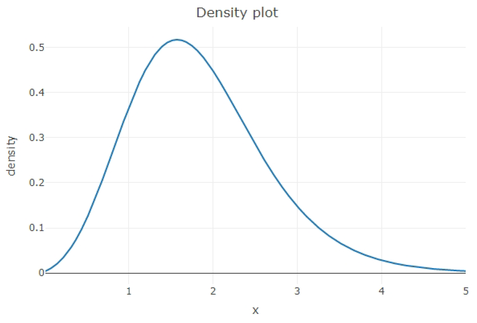
To compare the proposed methods, a numerical study was conducted in statistical software R [19], up to four digit accuracy. It is important to note that the shape of the posterior density function for all cases under consideration followed a similar uni-modal shape as the one presented in Figure 1. Therefore, using the nominal value $\alpha =0.05$, we obtained the $95\%$ Bayesian two-sided equi-tailed and HPD intervals for the order statistics from future samples of size $m=5,10$, and 20.

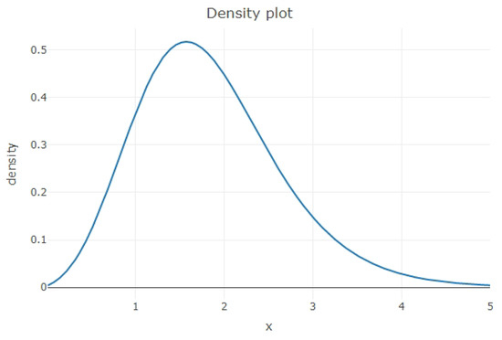
Figure 1. Posterior density function for Case I when $(m,j,k)=(10,9,1).$

The data analysis indicated that the corresponding Bayesian credible intervals differed notably when compared with the case of non-informative priors in the sense that they provided more accurate results. Furthermore, when the prior information became available, the width of the intervals decreased. Case III dominated in these circumstances, which was quite reasonable due to the mean and variance of the prior distribution for this case. Furthermore, the HPD method was seen to be more precise than the other method. However, it was seen that the HPD method had several drawbacks when considering the minimum of the sample as the size of the future sample increased. Therefore, the Bayesian equi-tailed interval was adopted as preferable for considerations in practice. Since the MSPEs of the point predictors depend on $\theta$, we evaluated the estimate of $\theta$ from (9). These results are presented in Table 1, Table 2, Table 3 and Table 4 for Cases I, II, and III and for the case of non-informative priors, respectively, when $k=1$ and 2.

Table 1. The 95% Bayesian prediction interval and point predictor for $Y_{j:m}$ of a future sample of size m when $(a,b)=(0.5,0.5)$. HPD, highest posterior density.

	m	j	Equi-Tailed (L)	HPD (L)	Point Predictor	${\displaystyle \widehat{\mathit{MSPE}}}$
$k=1$	5	1	(0.0002, 0.8441)(0.8439)	(0, 0.4078)(0.4078)	0.1979	0.3539
		4	(0.1518, 2.9883)(2.9883)	(0.0071, 2.5511)(2.544)	1.2169	1.0381
		5	(0.4213, 5.2704)(4.8491)	(0.1649, 4.6581)(4.4933)	2.1937	2.1237
	10	1	(0.0001, 0.4914)(0.4913)	(0, 0.152)(0.152)	0.1059	0.2134
		4	(0.0229, 1.2191)(1.1962)	(0.0114, 0.6015)(0.5901)	0.4488	0.4485
		9	(0.5101, 3.7272)(3.2171)	(0.3605, 3.4754)(3.1149)	1.843	1.1235
		10	(0.8827, 5.9623)(5.0795)	(0.6198, 5.4447)(4.825)	2.831	2.1681
	20	1	(0, 0.3007)(0.3007)	(1.0004, 1.9989)(0.9985)	0.0592	0.1422
		4	(0.0035, 0.6687)(0.6652)	(0.72, 2.0887)(1.3688)	0.1095	0.2697
		10	(0.0849, 1.3732)(1.2883)	(0.0194, 1.2548)(1.2354)	0.6277	0.4575
		18	(0.7677, 3.5322)(2.7645)	(0.6768, 3.4091)(2.7322)	2.0063	0.9099
		20	(1.4513, 6.6548)(5.2035)	(1.1921, 6.1853)(4.9932)	3.4943	2.1922
$k=2$	5	1	(0.0004, 0.7382)(0.738)	(0, 0.6065)(0.6065)	0.1664	0.9503
		4	(0.1544, 2.8678)(2.7134)	(0.021, 2.508)(2.487)	1.1481	4.3966
		5	(0.4156, 5.1632)(4.7475)	(0.1711, 4.5431)(4.3719)	2.1188	7.3214
	10	1	(0.0004, 0.4006)(0.4005)	(0, 0.1592)(0.1592)	0.0833	0.5601
		4	(0.0265, 1.0913)(1.0648)	(0.004, 0.5882)(0.5842)	0.4021	1.8838
		9	(0.5153, 3.605)(3.0897)	(0.367, 3.3418)(2.9748)	1.7666	5.9481
		10	(0.8751, 5.8549)(4.9798)	(0.6159, 5.3185)(4.7026)	2.7516	8.4322
	20	1	(0, 0.2271)(0.2271)	(0, 0.0171)(0.0171)	0.043	0.4344
		4	(0.0048, 0.5561)(0.5513)	(0, 0.5804)(0.5804)	0.1776	1.001
		10	(0.0966, 1.2327)(1.1362)	(0, 1.831)(1.831)	0.5684	2.52
		18	(0.782, 3.3997)(2.6178)	(0.686, 3.2627)(2.5767)	1.9287	6.0765
		20	(1.4425, 6.5473)(5.1048)	(1.1834, 6.0553)(4.8719)	3.4133	9.5048

Table 2. The 95% Bayesian prediction interval and point predictor for $Y_{j:m}$ of a future sample of size m when $(a,b)=(1,1)$.

	m	j	Equi-Tailed (L)	HPD (L)	Point Predictor	${\displaystyle \widehat{\mathit{MSPE}}}$
$k=1$	5	1	(0.0002, 0.8366)(0.8364)	(0, 0.4079)(0.4079)	0.1587	0.4678
		4	(0.1642, 2.9848)(2.8206)	(0.0177, 2.6214)(2.6037)	1.2222	1.3447
		5	(0.4395, 5.2719)(4.8324)	(0.1854, 4.6633)(4.4779)	2.2024	2.4408
	10	1	(0.0001, 0.4832)(0.4831)	(0, 0.1464)(0.1464)	0.1053	0.2956
		4	(0.0274, 1.2083)(1.181)	(0.0073, 0.657)(0.6497)	0.4552	0.6576
		9	(0.5335, 3.7237)(3.1902)	(0.3848, 3.472)(3.0872)	1.8502	1.4587
		10	(0.9072, 5.9637)(5.0565)	(0.6453, 5.4435)(4.7982)	2.8392	2.5194
	20	1	(0, 0.2931)(0.2931)	(0, 0.0271)(0.0271)	0.0579	0.1985
		4	(0.0047, 0.6569)(0.6522)	(0, 0.491)(0.491)	0.2146	0.4057
		10	(0.0966, 1.3597)(1.2631)	(0, 0.9271)(0.9271)	0.6309	0.694
		18	(0.7977, 3.5255)(2.7278)	(0.706, 3.4001)(2.6941)	2.0138	1.2505
		20	(1.4795, 6.6562)(5.1767)	(1.2203, 6.1813)(4.961)	3.5031	2.5501
$k=2$	5	1	(0.0003, 0.7386)(0.7383)	(0, 0.3248)(0.3248)	0.1682	0.9574
		4	(0.1633, 2.8722)(2.7089)	(0.03, 2.5178)(2.4878)	1.1558	4.3035
		5	(0.429, 5.1705)(4.7415)	(0.1853, 4.553)(4.3677)	2.1285	6.8663
	10	1	(0.0001, 0.3996)(0.3994)	(0, 0.0837)(0.0.0837)	0.0841	0.5643
		4	(0.0299, 1.0902)(1.0603)	(0.0021, 0.6624)(0.6603)	0.4062	1.8799
		9	(0.532, 3.6094)(3.0774)	(0.3844, 3.3467)(2.9623)	1.7762	5.6689
		10	(0.8932, 5.8623)(4.9691)	(0.6347, 5.3249)(4.6903)	2.7622	7.7939
	20	1	(0.0001, 0.2256)(0.2255)	(0, 0.0085)(0.0085)	0.0434	0.3443
		4	(0.0058, 0.5532)(0.5475)	(0, 0.3071)(0.3071)	0.1796	1.0142
		10	(0.1053, 1.2299)(1.1246)	(0, 0.9707)(0.9707)	0.574	2.4084
		18	(0.8032, 3.4023)(2.599)	(0.707, 3.2642)(2.5571)	1.9387	5.6668
		20	(1.4634, 6.5547)(5.0913)	(1.2044, 6.06)(4.8556)	3.4244	9.0046

Table 3. The 95% Bayesian prediction interval and point predictor for $Y_{j:m}$ of a future sample of size m when $(a,b)=(2,2)$.

	m	j	Equi-Tailed (L)	HPD (L)	Point Predictor	${\displaystyle \widehat{\mathit{MSPE}}}$
$k=1$	5	1	(0.0004, 0.8245)(0.8241)	(0, 0.4076)(0.4076)	0.1983	0.5943
		4	(0.1848, 2.9793)(2.7945)	(0.0426, 2.6312)(2.5887)	1.2306	1.6946
		5	(0.4685, 5.2742)(4.8057)	(0.2178, 4.6699)(4.452)	2.2139	2.8466
	10	1	(0.0004, 0.4698)(0.4697)	(0, 0.137)(0.137)	0.1048	0.3808
		4	(0.0356, 1.1906)(1.1551)	(0.0032, 0.7704)(0.7672)	0.4582	0.8932
		9	(0.5709, 3.7181)(3.1472)	(0.4236, 34657)(3.0422)	1.8608	1.8736
		10	(0.9457, 5.9661)(5.0203)	(0.6855, 5.4411)(4.7556)	2.8521	2.9438
	20	1	(0.0001, 0.2805)(0.2804)	(0, 0.0218)(0.0218)	0.0572	0.2559
		4	(0.0072, 0.6373)(0.6302)	(0, 0.4761)(0.4601)	0.2146	0.5685
		10	(0.1172, 1.3372)(1.22)	(0, 0.9402)(0.9402)	0.6358	0.9711
		18	(0.8455, 3.5147)(2.6692)	(0.7525, 3.3851)(2.6327)	2.0257	1.6483
		20	(1.5235, 6.6586)(5.1351)	(1.2645, 6.1749)(4.9103)	3.5167	3.0199
$k=2$	5	1	(0.0004, 0.7391)(0.7387)	(0, 0.3311)(0.3311)	0.1712	0.9406
		4	(0.1789, 2.8797)(2.7008)	(0.0457, 2.5329)(2.4873)	1.169	3.9559
		5	(0.4517, 5.183)(4.7312)	(0.2092, 4.569)(4.3599)	2.1449	6.3233
	10	1	(0.0001, 0.3976)(0.3975)	(0, 0.0825)(0.0825)	0.0856	0.5619
		4	(0.0362, 1.0882)(1.052)	(0.0003, 0.784)(0.7836)	0.4133	1.8005
		9	(0.5605, 3.6169)(3.0564)	(0.4138, 3.3547)(2.9409)	1.7923	5.1354
		10	(0.9235, 5.8747)(4.9512)	(0.6661, 5.3355)(4.6694)	2.78	7.1274
	20	1	(0.0001, 0.2228)(0.2227)	(0, 0.0076)(0.0076)	0.044	0.3505
		4	(0.0078, 0.5481)(0.5403)	(0, 0.306)(0.306)	0.1831	1.001
		10	(0.1211, 1.2248)(1.1037)	(0, 0.9725)(0.9725)	0.5834	2.3601
		18	(0.8392, 3.4065)(2.5673)	(0.7426, 3.2664)(2.5238)	1.9556	5.3681
		20	(1.4982, 6.5671)(5.069)	(1.2396, 6.0678)(4.8282)	3.4431	8.1053

Table 4. The 95% Bayesian prediction interval and point predictor for $Y_{j:m}$ of a future sample of size m when $(a,b)=(0,0)$.

	m	j	Equi-Tailed (L)	HPD (L)	Point Predictor	${\displaystyle \widehat{\mathit{MSPE}}}$
$k=1$	5	1	(0.0001, 0.8527)(0.8526)	(0, 0.4075)(0.4075)	0.1977	0.4131
		4	(0.1376, 2.9923)(2.8548)	(0.0097, 2.4327)(2.423)	1.2106	0.9424
		5	(0.3998, 5.2686)(4.8689)	(0.1401, 4.6506)(4.5105)	2.1864	1.9324
	10	1	(0.0001, 0.501)(0.5009)	(0, 0.1583)(0.1583)	0.1064	0.3042
		4	(0.0184, 1.2316)(1.2132)	(0.0174, 0.5405)(0.5231)	0.4512	0.4798
		9	(0.4826, 3.7313)(3.2488)	(0.3315, 3.4788)(3.1473)	1.8341	1.0576
		10	(0.8534, 5.9605)(5.1071)	(0.5891, 5.4459)(4.8568)	2.8212	1.9971
	20	1	(0, 0.3096)(0.3096)	(0, 0.0349)(0.0349)	0.0595	0.1999
		4	(0.0025, 0.6823)(0.6798)	(0, 0.5055)(0.5055)	0.2141	0.2011
		10	(0.0723, 1.3888)(1.3165)	(0, 0.9072)(0.9072)	0.6243	0.2287
		18	(0.7322, 3.54)(2.8078)	(0.6422, 3.4193)(2.7771)	1.9972	0.8487
		20	(1.4174, 6.653)(5.2356)	(1.1582, 6.1899)(5.0317)	3.4839	1.9905
$k=2$	5	1	(0.0001, 0.7377)(0.7376)	(0, 0.317)(0.317)	0.1645	1.092
		4	(0.1445, 2.8628)(2.7183)	(0.0105, 2.4955)(2.485)	1.1392	4.5601
		5	(0.4006, 5.1548)(4.7542)	(0.1552, 4.5314)(4.3762)	2.1077	7.4088
	10	1	(0.0001, 0.4018)(0.4017)	(0, 0.0849)(0.0849)	0.0823	0.5972
		4	(0.023, 1.0925)(1.0694)	(0.0051, 0.5453)(0.5402)	0.3975	1.9586
		9	(0.4964, 3.5999)(3.1035)	(0.3474, 3.336)(2.9886)	1.7557	6.4913
		10	(0.8546, 5.8465)(4.9919)	(0.5947, 5.3111)(4.7165)	2.7395	8.9099
	20	1	(0, 0.2288)(0.2288)	(0, 0.0097)(0.0097)	0.0426	0.3672
		4	(0.0038, 0.5591)(0.5553)	(0, 0.3072)(0.3072)	0.1754	1.5641
		10	(0.0873, 1.2357)(1.1485)	(0,0.9673)(0.9673)	0.5622	2.5221
		18	(0.7579, 3.3968)(2.6389)	(0.6621, 3.2609)(2.5987)	1.9173	6.318
		20	(1.4187, 6.5389)(5.1202)	(1.1594, 6.0499)(4.8905)	3.4007	10.2724

MSPEs were increasing with respect to k, while the equi-tailed credible interval width was decreasing with respect to k. Case III did not dominate other cases. Case III did not have the smallest values of the MSPEs, and it did not have the shortest intervals everywhere. In the most cases, the HPD intervals were shorter than the equi-tailed ones.

6. Conclusions

In this paper, we addressed the problem of presenting Bayesian point predictors of order statistics of a future sample of size m based on the $k^{\mathrm{th}}$ lower record values from a GED. With respect to the SEL, we investigated the point prediction of order statistics from a future sample. Furthermore, we presented the construction of Bayesian and HPD intervals. An illustrative example was given to show the implementation of the procedures developed.

It may be interesting to compare point predictors for order statistics based on lower record values from GED with those point predictors of order statistics when upper record values are observed from the exponential distribution. This may motivate researchers to transform data from the exponential distribution to the GED in order to obtain better point predictors.

References

- Chandler, K.N. The distribution and frequency of record values. J. R. Stat. Soc. Ser. (Methodol.) 1952, 14, 220–228. [Google Scholar] [CrossRef]
- Balakrishnan, N.; Arnold, B.C.; Nagaraja, H.N. Records; Wiley: Hoboken, NJ, USA, 1998. [Google Scholar]
- Nevzorov, V.B. Records: Mathematical Theory; Translations of Mathematical Monographs; AMS: Providence, RI, USA, 2000. [Google Scholar]
- Arnold, B.C.; Balakrishnan, N.; Nagaraja, H.N. A First Course in Order Statistics; SIAM: Philadelphia, PA, USA, 2008. [Google Scholar]
- David, H.A.; Nagaraja, H.N. Order Statistics; John Wiley & Sons, Inc.: Hoboken, NJ, USA, 2003. [Google Scholar]
- Ahsanullah, M. Linear prediction of record values for the two parameter exponential distribution. Ann. Inst. Stat. Math. 1980, 32, 363–368. [Google Scholar] [CrossRef]
- Ahmad, A.A.; Raqab, M.Z.; Madi, M.T. Bayesian prediction intervals for future order statistics from the generalized exponential distribution. J. Iran. Stat. Soc. 2007, 6, 17–30. [Google Scholar]
- Ahmadi, J.; Balakrishnan, N. Prediction of order statistics and record values from two independent sequences. Statistics 2010, 44, 417–430. [Google Scholar] [CrossRef]
- Ahmadi, J.; MirMostafaee, S.M.T.K.; Balakrishnan, N. Bayesian prediction of order statistics based on k-record values from exponential distribution. Statistics 2011, 45, 375–387. [Google Scholar] [CrossRef]
- Gupta, R.D.; Kundu, D. Theory & methods: Generalized exponential distributions. Aust. N. Z. J. Stat. 1999, 41, 173–188. [Google Scholar]
- Gupta, R.D.; Kundu, D. Closeness of gamma and generalized exponential distribution. Commun. -Stat.-Theory Methods 2003, 32, 705–721. [Google Scholar] [CrossRef]
- Gupta, R.D.; Kundu, D. Discriminating between Weibull and generalized exponential distributions. Comput. Stat. Data Anal. 2003, 3, 179–196. [Google Scholar] [CrossRef]
- Raqab, M.M.; Ahsanullah, M. Estimation of the location and scale parameters of generalized exponential distribution based on order statistics. J. Stat. Comput. Simul. 2001, 69, 109–123. [Google Scholar] [CrossRef]
- Jaheen, Z.F. Empirical Bayes inference for generalized exponential distribution based on records. Commun.-Stat.-Theory Methods 2004, 33, 1851–1861. [Google Scholar] [CrossRef]
- Raqab, M.Z. Generalized exponential distribution: moments of order statistics. Statistics 2004, 38, 29–41. [Google Scholar] [CrossRef]
- Chen, M.H.; Shao, Q.M. Monte Carlo estimation of Bayesian credible and HPD intervals. J. Comput. Graph. Stat. 1999, 8, 69–92. [Google Scholar]
- Gradshteyn, I.S.; Ryzhik, I.M. Table of Integrals, Series, and Products; Academic Press: Cambridge, MA, USA, 2014. [Google Scholar]
- Asgharzadeh, A.; Valiollahi, R.; Raqab, M.Z. Estimation of Pr(Y<X) for the two-parameter generalized exponential records. Commun. -Stat.-Simul. Comput. 2017, 46, 379–394. [Google Scholar]
- R Core Team. R: A Language and Environment for Statistical Computing; R Foundation for Statistical Computing: Vienna, Austria, 2015. [Google Scholar]
© 2019 by the author. Licensee MDPI, Basel, Switzerland. This article is an open access article distributed under the terms and conditions of the Creative Commons Attribution (CC BY) license (http://creativecommons.org/licenses/by/4.0/).