Article

Evaluating the Performance of Multiple Imputation Methods for Handling Missing Values in Time Series Data: A Study Focused on East Africa, Soil-Carbonate-Stable Isotope Data

1
Research Institute of Energy Management and Planning (RIEMP), University of Tehran, Tehran 1417466191, Iran
2
Department of Statistics, Payame Noor University, Tehran 19395-4697, Iran
3
PHASTAR, London W4 5LE, UK
*
Author to whom correspondence should be addressed.
Stats 2019, 2(4), 457-467; https://doi.org/10.3390/stats2040032
Submission received: 18 November 2019 / Revised: 7 December 2019 / Accepted: 11 December 2019 / Published: 16 December 2019

Abstract

:
In all fields of quantitative research, analysing data with missing values is an excruciating challenge. It should be no surprise that given the fragmentary nature of fossil records, the presence of missing values in geographical databases is unavoidable. As in such studies ignoring missing values may result in biased estimations or invalid conclusions, adopting a reliable imputation method should be regarded as an essential consideration. In this study, the performance of singular spectrum analysis (SSA) based on L 1 norm was evaluated on the compiled δ 13 C data from East Africa soil carbonates, which is a world targeted historical geology data set. Results were compared with ten traditionally well-known imputation methods showing L 1 -SSA performs well in keeping the variability of the time series and providing estimations which are less affected by extreme values, suggesting the method introduced here deserves further consideration in practice.

1. Introduction

Handling missing values is a common challenge in almost all areas of study: from economics and social sciences to geology, archaeology and medicine [1,2,3]. As the primary aim of any data collection process is to obtain a more profound domain knowledge, the presence of missing values which causes failure in “complete-case” analysis is clearly undesirable.
Although almost all quantitative studies are affected by incomplete data, missing values are particularly prominent in longitudinal data. In this study, we introduce a new method of missing values imputation using a non-parametric time series analysis technique: singular spectrum analysis (SSA). Imputing missing values using this relatively new but powerful time series analysis method was expected to provide analytical improvements, which are discussed in the subsequent sections.
We used the East Africa soil-carbonate-stable isotope ( δ 13 C ) dataset, which is an excellent example of a widely used dataset with large proportions of missing data. East Africa soil-carbonate-stable isotope ( δ 13 C ) was collected from multiple sites of Ethiopia, Kenya and Tanzania, and later compiled by Levin in 2013 [4] (see Figure 1). The stable carbon isotopic has been widely used in archaeology to infer paleodiet, artefact provenance, and paleoenvironment [5]. The presence of considerable missing values in this data introduces an element of ambiguity into inferential analysis by affecting properties of statistical estimators such as variance or periodicity.
Also, as discussed in several studies, ignoring missing values of the East Africa soil-carbonate-stable isotope ( δ 13 C ) or other similar datasets may lead to misinterpretation of macroevolutionary patterns [6], drawing inaccurate connections existed among lineages [7] or even invalid timing estimation of diversification events [6].
In this study, a comparison was performed on several imputation techniques and the estimated values produced by SSA. We first provide a brief introduction to SSA and its characteristics which make it a suitable candidate for imputing missing values in such a powerful and prominent archaeological time series data with the oldest observation related to four million years ago. We will then briefly discuss the selection of methods which have been applied to deal with this problem.
Our results suggest that the newly introduced method based on SSA technique produces a robust estimation of missing values and deserves further consideration in practice.
The remainder of this paper is organised such that Section 2 presents an outline of the steps underlying the SSA techniques and describes the newly introduced approach. Section 3 provides an overview of the other imputation techniques evaluated in this study. Section 4 explains the data under study, and in Section 5, the results obtained using the East Africa soil-carbonate-stable isotope data are discussed. The paper concludes with a concise summary in Section 6.

2. Review of SSA

The SSA technique includes two complementary stages: decomposition and reconstruction, each of which consists of two separate steps. The first stage decomposes a time series into several components that allows for signal extraction and noise reduction. The reconstruction stage leads to a less noisy series using the leading eigentriples of the trajectory matrix. The most common version of SSA is called basic SSA. It is noteworthy that the matrix norm used in basic SSA is the Frobenius norm or L 2 -norm. A newer version of SSA which is based on L 1 -norm, and is therefore, called L 1 -SSA, has been introduced and further explained in [8,9]; and it has been confirmed that L 1 -SSA is robust against outliers. In the following, the steps of these two versions of SSA are concisely presented and differences highlighted. The theory underlying basic SSA is explained in detail in [10]. For more detailed information on L 1 -SSA, see [8].
Stage 1: Decomposition (Embedding and Singular Value Decomposition)
In embedding step, the time series Y N = { y 1 , , y N } is mapped into the vectors X 1 , , X K where X i = ( y i , , y i + L 1 ) T and K = N L + 1 . The single choice of this step is the integer number L such that 2 L N 1 called window length. The output of the embedding step is the trajectory matrix X = [ X 1 : : X K ] whose columns are the vectors X i . The trajectory matrix is a Hankel matrix in the sense that all elements on the anti-diagonal are equal.
In the singular value decomposition (SVD) step, the SVD of the trajectory matrix X is performed. The eigenvalues of X X T and corresponding eigenvectors are denoted by λ 1 , , λ L (in decreasing order of magnitude) and ( U 1 , , U L ) . If d = max { i , such that λ i > 0 } = r a n k ( X ) , then the SVD of the trajectory matrix in basic SSA can be written as X = X 1 + + X d , where X i = λ i U i V i T and V i = X T U i / λ i ( i = 1 , , d ). The collection ( λ i , U i , V i ) is called ith eigentriple of the SVD.
In L 1 -SSA, the matrices X i have the form X i = w i λ i U i V i T where w i is the weight of singular value λ i . These weights are diagonal elements of the diagonal weight matrix W = d i a g ( w 1 , w 2 , , w d , 0 , 0 , , 0 ) and are computed such that X U W Σ V T L 1 is minimised; where U = [ U 1 : : U L ] , V = [ V 1 : : V L ] , Σ = d i a g ( λ 1 , λ 2 , , λ L ) and . L 1 is the L 1 norm of a matrix. For more information, see [8].
Stage 2: Reconstruction (Grouping and Hankelization)
In the grouping step, the set of indices { 1 , , d } is partitioned into m disjoint subsets I 1 , , I m . The matrix X I corresponding to the group I is defined as X I = X i 1 + + X i p where I = { i 1 , , i p } . For example, if I = { 2 , 5 , 6 } , then X I = X 2 + X 5 + X 6 . After computing that matrices for the groups I = I 1 , , I m , the SVD of X can be written as
X = X I 1 + + X I m .
In Hankelization step, we seek to transform each matrix X I of the grouping step into a Hankel matrix so that these can subsequently be converted into a time series by combining the first column (row) and the last row (column) of the Hankel matrix. In basic SSA, Hankelization is obtained via diagonal averaging of the matrix elements over the anti-diagonals. Let A be an L × K matrix with elements a i j , 1 i L , 1 j K . By diagonal averaging, the matrix A is transferred into the Hankel matrix H A with the elements a ˜ s over the anti-diagonals ( 1 s N ) using the following formula:
a ˜ s = ( l , k ) A s a l k | A s | ,
where A s = { ( l , k ) : l + k = s + 1 , 1 l L , 1 k K } and | A s | denotes the number of elements in the set A s . By applying diagonal averaging (2) to all the matrix components of (1), the following expansion is obtained: X = X ˜ I 1 + + X ˜ I m , where X ˜ I j = H X I j , j = 1 , , m . In L 1 -SSA, Hankelisation corresponds to computing the median of the matrix elements over the anti-diagonals [8].
Imputation Based on SSA
Generally, in the iterative SSA imputation method, first, missing values are replaced by initial values, and then reconstructed repeatedly until convergence occurs [11]. The last reconstructed values are considered imputed values. This imputation algorithm contains the following steps:
  • Set suitable initial values in place of missing data (e.g., mean of the non missing data).
  • Choose reasonable values of window length (L) and the number of leading eigentriples (r).
  • Reconstruct the time series where its missing data are replaced with initial values.
  • Replace the values of time series at missing locations with their reconstructed values.
  • Reconstruct the time series.
  • Repeat steps 4 and 5 until the maximum absolute value of the difference between consecutive replaced values of the time series by their reconstructed value is less than δ ( δ is the convergence threshold and is a small positive number).
  • Consider the final values replaced to be the imputed values.
It is noticeable that the SSA-based imputation can be performed via basic SSA or L 1 -SSA. We applied both basic SSA and L 1 -SSA to impute missing values in this investigation. It is worth mentioning that the mean of the non-missing data was utilised as an initial value for a missing data and not the final estimate. In the iterative SSA algorithm, initial values are replaced with reconstructed value until convergence occurs.

3. Other Imputation Methods

The other imputation algorithms of univariate time series which were used in this study are as follows:
  • Interpolation: linear, spline and Stineman interpolation.
  • Kalman smoothing (ARIMA): the Kalman smoothing on the state space representation of an ARIMA model.
  • Kalman smoothing (StructTS): the Kalman smoothing on structural time series models fitted by maximum likelihood.
  • Last observation carried forward (LOCF): each missing value is replaced with the most recent present value prior to it.
  • Next observation carried backward (NOCB): the LOCF is done from the reverse direction, starting from the back of the series.
  • Weighted moving average: Missing values are replaced by weighted moving average values. The average in this implementation is taken from an equal number of observations on either side of a missing value. For example, to impute a missing value at location i, the observations y i 2 , y i 1 , y i + 1 , y i + 2 , are used to calculate the mean for moving average window size 4 (2 left and 2 right). Whenever all observations in the current window are not available (NA), the window size is incrementally increased until there are at least 2 non-NA values present. The weighted moving average is used in the following three ways:
    • Simple moving average (SMA): all observations in the moving average window are equally weighted for calculating the mean.
    • Linear weighted moving average (LWMA): Weights decrease in arithmetical progression. The observations directly next to the ith missing value ( y i 1 , y i + 1 ) have weight 1/2, the observations one further away ( y i 2 , y i + 2 ) have weight 1/3, the next y i 3 , y i + 3 have weight 1/4 and so on. This method is the variation of inverse distance weighting.
    • Exponential weighted moving average (EWMA): Weights decrease exponentially. The observations directly next to the ith missing value have weight 1 2 1 , the observations one further away have weight 1 2 2 , the next have weight 1 2 3 and so on. This method is also the variation of inverse distance weighting.
In this study, we use the moving average with a window of size 8 (4 left and 4 right). For SSA-based imputation methods, the R package Rssa was employed together with the R scripts generated by the authors. For more information on Rssa see [12,13,14]. All calculations of other imputation methods were done with the help of the R package of imputeTS [15]. More detailed information about the theoretical background of the algorithms such as interpolation and Kalman smoothing can be found in the imputeTS manual [16]. Kalman smoothing (or the Kalman filter) is a well-known method of time series analysis and it is not the smoothing part of interpolation.

4. Data

East Africa soil-carbonate-stable isotope data, compiled by Levin [4], has been widely used as a valuable source of information for various research communities [4,17,18,19]. When compiling the data, the δ 13 C was measured against the Vienna Pee Dee Belemnite (VPDB) per millilitre (%) [4]. The compilation does not include data from non-pedogenic carbonates. Age is reported in Ma (millions of years ago) (For more information regarding the age calculation method see [4]). It is evident, while attempts have been made for this compilation to be as complete as possible, the published dataset contains large proportions of missing data. Also, the length of the original series was reduced from 1360 observations to 491 (including missing values) because multiple pedogenic carbonate nodules reported from a single soil outcrop (~ 1   m 2 ) were replaced by their average value.
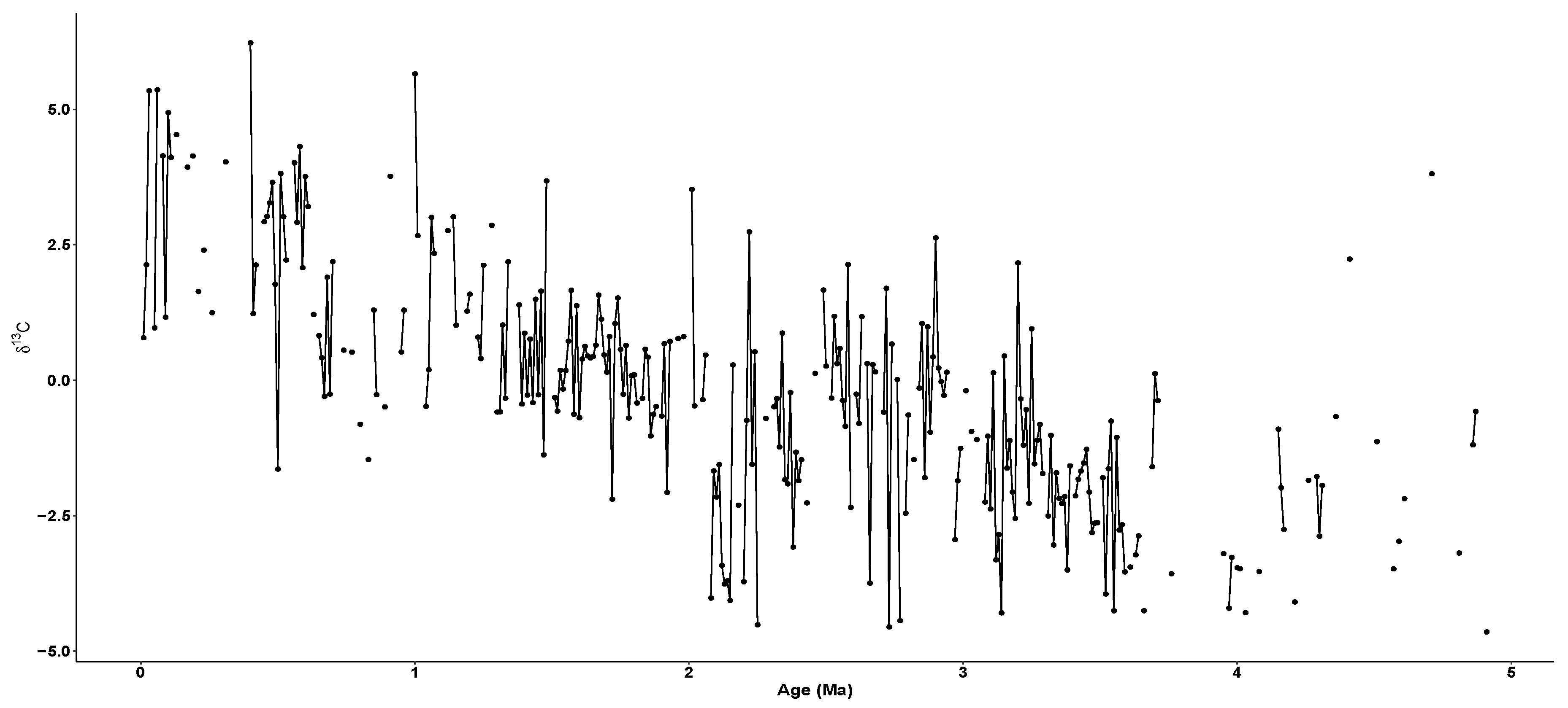
Figure 2 illustrates a plot of averaged δ 13 C values against age (black points). δ 13 C values range from −4.65 (%) to +6.23 (%) and ages are assigned as in [4]. To identify the location of missing values in the time series, a time interval of 0.02 Ma is considered and ages without a reported δ 13 C value are marked as missing values.
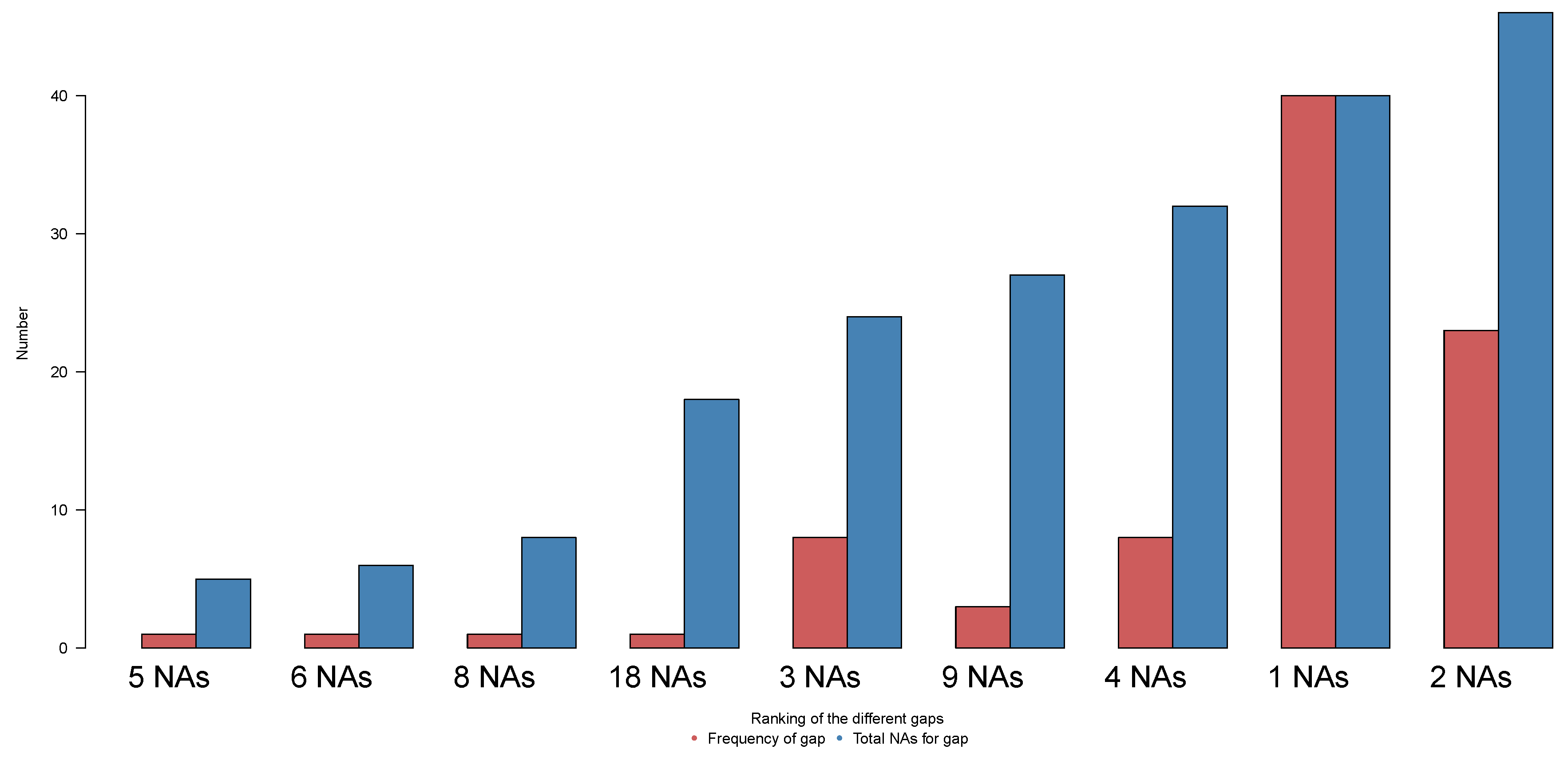
The length of this data set is 491 and the number of NAs is 206. Hence, 42% of measurements are missing. Figure 3 shows the length of NA gaps (consecutive NAs) in the time series and presents a ranking of which gaps occur most often. The frequency of each gap and the associated number of NAs of that gap are also reported in that figure. For example, the gap of length two (2NAs) occurs 23 times, making up for overall 46 NAs; the gap of length three (3NAs) occurs eight times, making 24 NAs totally; and so on. The most frequent gap is of length one, occurring 40 times, and the longest gap has size 18.

5. Imputing Results

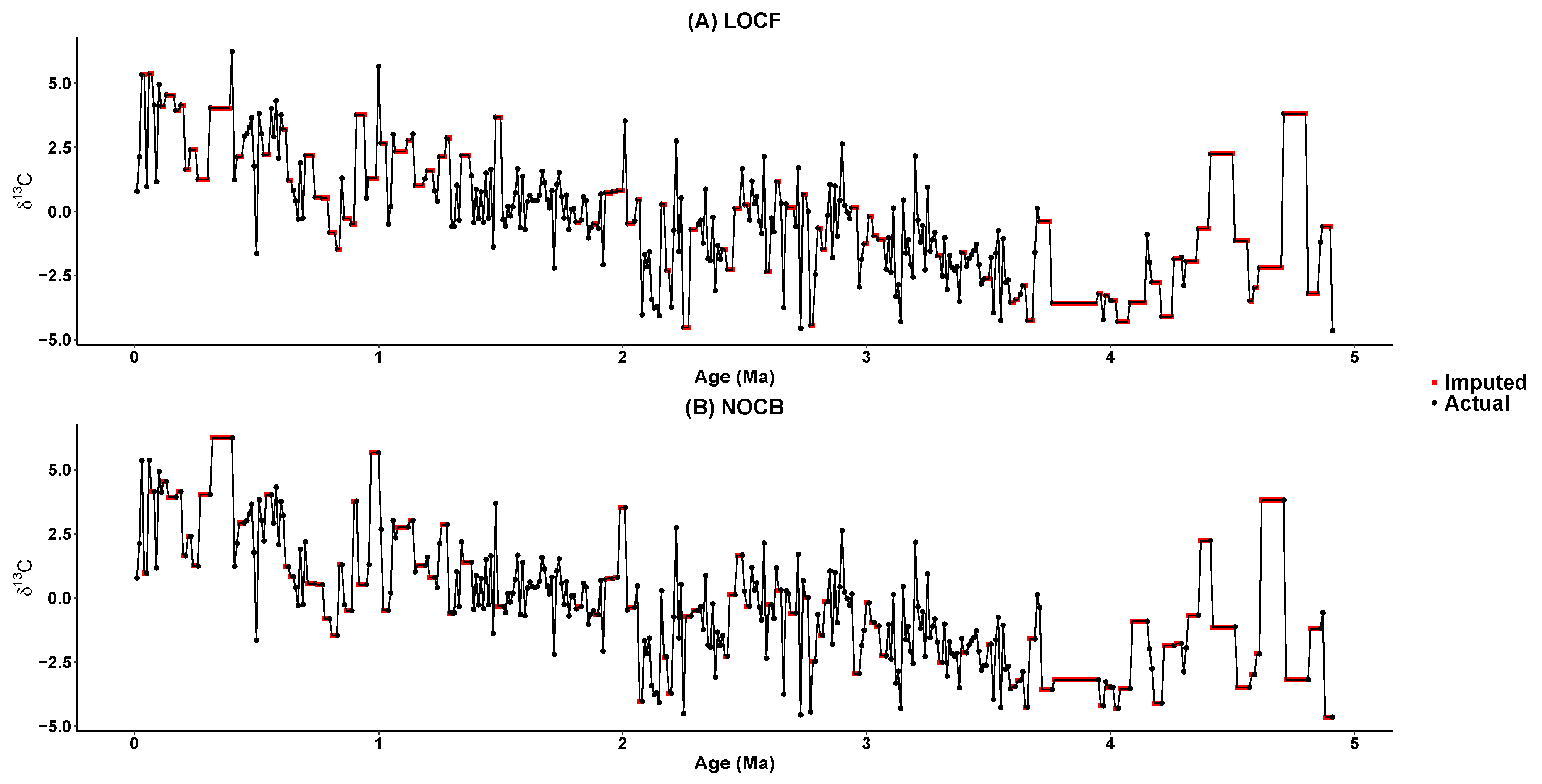
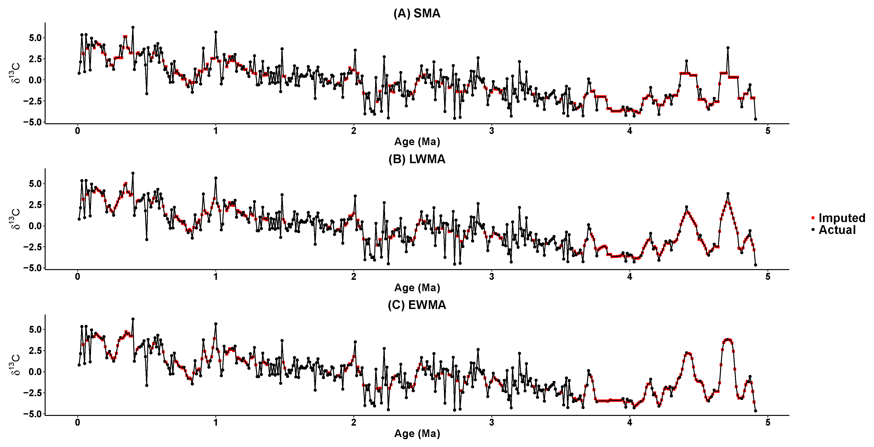
Figure 4, Figure 5, Figure 6, Figure 7 and Figure 8 depict the application of imputation methods adopted in this study where the imputed values are shown in red.
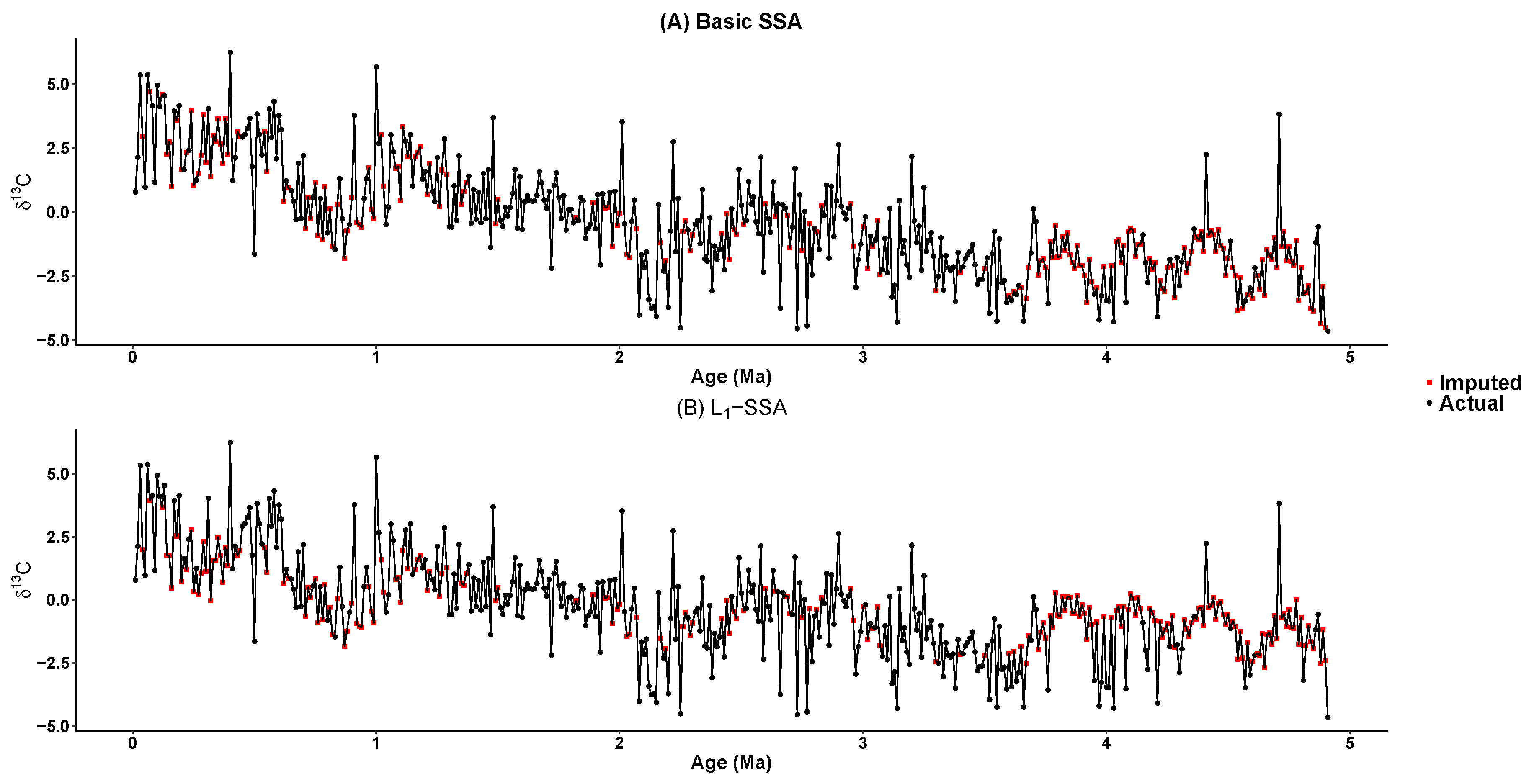
Figure 4 shows the results achieved by basic SSA and L 1 -SSA respectively. Note how the imputed values are not only consistent with the general pattern of the data, but also contain volatility with an amount similar to what is present in data without NAs, thereby providing the reader with a trusty outlook for the long-term prospects of the soil carbonate time series.
The window length (L) and the number of leading eigentriples (r) are two important parameters in SSA. It is well know that the performance of the imputation depends crucially on these parameters. In the case of no missing data, the general recommendation is to choose the window length close to half of the series length [20]. By replacing missing data with the mean of the non missing data and following the recommendations in [20], we chose L = 245 . In order to choose r, the information contained in singular values and singular vectors of the trajectory matrix of the time series must be be used. In doing so, a scree plot of the singular values, one-dimensional and two-dimensional figures of the singular vectors, and the matrix of the absolute values of the weighted correlations can provide a visual method to select r [21,22]. The analysis of the eigenvectors showed that the eigenvectors with indices from 1 to 16 correspond to the signal and all the rest may be classified as being produced by noise. Therefore, we chose r = 16 in order to reconstruct the time series. More information on choosing parameters L and r can be found in [23,24,25,26].
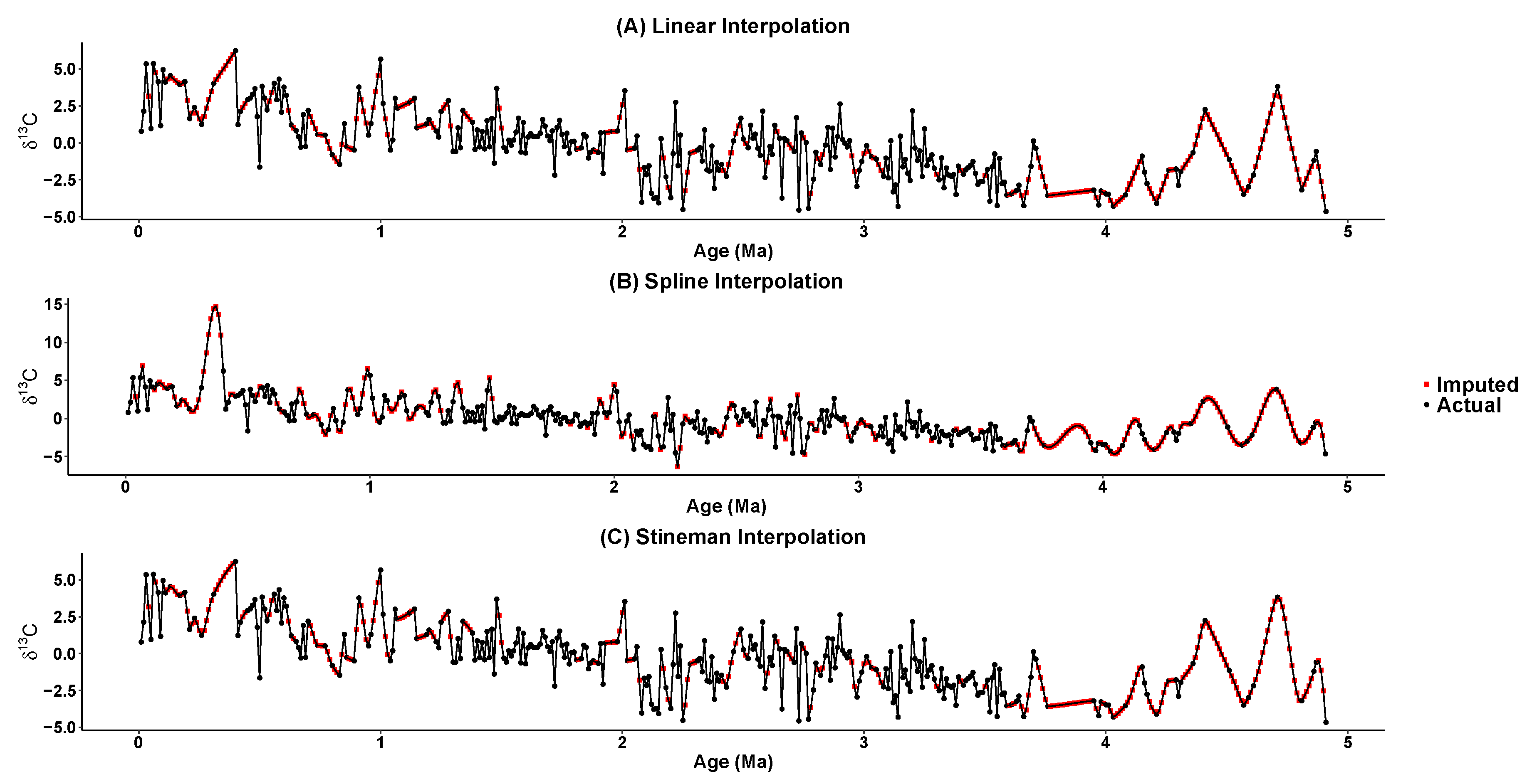
In Figure 5, imputed values generate a smooth line. The interpolation methods appear to have difficulties in accurately capturing the variation when they are faced with a significant number of missing values, as is clearly visible within the last 30% of the data.
The values imputed by Kalman Smoothing in Figure 6 are not significantly affected by extreme δ 13 C values; hence, leaving a series which appears to have a number of peak values. This is important as the complete-case analysis on the data may result in misleading conclusions by easily detecting those points as outliers. Thus, those points should not be considered outliers.
It appears from Figure 7 that the LOCF and NOCB methods can be improved to provide better estimates, as all imputed values are equal in a particular gap when LOCF (or NOCB) is employed. We consider this aspect further in the discussion which follows.
As visual inspections fall short of providing sound evidence, to compare the different imputing methods, statistical properties of the original and imputed time series are presented in Table 1.
To have a comprehensive view of different imputing methods employed here, the entire dataset was treated as the main source. Then, 10% to 40% of the dataset was randomly deleted and removed from the time series. Those missing data were then estimated with an imputing algorithm. The mean squared error (MSE) was utilised as the main criterion to compare the performances of the imputing algorithms. The mean values of MSEs are reported in Table 2, obtained from 1000 replications, for various levels of missing values (10% to 40%). The results confirm that the SSA-based approach works well. In addition, it can be concluded that the LOCF and NOCB methods have poor performance compared to other imputing techniques.

6. Conclusions

Following the recent theoretical and empirical success of L 1 -SSA at providing more reliable reconstructions and forecasts in comparison to basic SSA, in this study, the application of a number of imputation methods, including L 1 -SSA, was evaluated. We initially explained the SSA technique and produced an outline of the algorithms for imputing missing values based on L 1 -SSA. In brief, to estimate a missing value in a time series, the algorithm is optimised based on minimising the difference between consecutively replaced value and the attributed reconstructed one.
We compared the performances of SSA-based methods and interpolation, Kalman smoothing, LOCF, NOCB and weighted moving average approaches. It is noteworthy that we analysed them with 1D imputation. In addition to the descriptive analyses reported in the previous section, the results of cross-validation are also provided. The results yet again indicate the superiority of the SSA-based models over other methods considered here for various levels of missing values.
As confirmed by the measures of central tendency, the introduced approach of missing values processing is undoubtedly a practical benefit, in particular to those researchers working with time series datasets with significant missing values. As was mentioned before, SSA is a non-parametric time series analysis and signal processing technique which does not rely on any assumptions. Therefore, it can practically lend itself as an imputation method to other types of datasets.

Author Contributions

Conceptualization, H.H., M.K. and Z.G.; Investigation, H.H., M.K. and Z.G.; Methodology, H.H., M.K. and Z.G.; Supervision, H.H.; Writing—review & editing, H.H., M.K. and Z.G.

Funding

This research received no external funding.

Acknowledgments

The authors would like to thank the editor and anonymous referees for their invaluable comments, feedback and suggestions which helped improve the quality of this manuscript. Our heartfelt gratitude to the referees whose comments were very helpful in contributing to a major improvement in the revised version.

Conflicts of Interest

The authors declare that they have no conflict of interest.

Abbreviations

The following abbreviations are used in this manuscript:
SSAsingular spectrum analysis
SVDsingular value decomposition
NAnot available
ARIMAautoregressive integrated moving average
LOCFlast observation carried forward
NOCBnext observation carried backward
SMAsimple moving average
LWMAlinear weighted moving average
EWMAexponential weighted moving average

References

  1. Kossinets, G. Effects of missing data in social networks. Soc. Netw. 2006, 28, 247–268. [Google Scholar] [CrossRef] [Green Version]
  2. Donders, A.R.T.; Van Der Heijden, G.J.; Stijnen, T.; Moons, K.G. A gentle introduction to imputation of missing values. J. Clin. Epidemiol. 2006, 59, 1087–1091. [Google Scholar] [CrossRef] [PubMed]
  3. Montanari, A.; Mignani, S. Notes on the bias of dissimilarity indices for incomplete data sets: The case of archaelogical classification. Qüestiió Quaderns D’EstadíStica i Investigació Operativa 1994, 18, 39–49. [Google Scholar]
  4. Levin, N.E. Compilation of East Africa Soil Carbonate Stable Isotope Data. In Interdisciplinary Earth Data Alliance (IEDA); 2013; Available online: http://dx.doi.org/10.1594/IEDA/100231 (accessed on 2 November 2018).
  5. Holliday, V.T.; Gartner, W.G. Methods of soil P analysis in archaeology. J. Archaeol. Sci. 2007, 34, 301–333. [Google Scholar] [CrossRef]
  6. Guillerme, T.; Cooper, N. Effects of missing data on topological inference using a Total Evidence approach. Mol. Phylogenet. Evol. 2016, 94, 146–158. [Google Scholar] [CrossRef] [PubMed]
  7. Manos, P.S.; Soltis, P.S.; Soltis, D.E.; Manchester, S.R.; Oh, S.H.; Bell, C.D.; Dilcher, D.L.; Stone, D.E. Phylogeny of extant and fossil Juglandaceae inferred from the integration of molecular and morphological data sets. Syst. Biol. 2007, 56, 412–430. [Google Scholar] [CrossRef] [PubMed] [Green Version]
  8. Kalantari, M.; Yarmohammadi, M.; Hassani, H. Singular Spectrum Analysis Based on L1-norm. Fluct. Noise Lett. 2016, 15, 1650009. [Google Scholar] [CrossRef]
  9. Kwak, N. Principal component analysis based on L1-norm maximization. IEEE Trans. Pattern Anal. Mach. Intell. 2008, 30, 1672–1680. [Google Scholar] [CrossRef] [PubMed]
  10. Silva, E.S.; Hassani, H. On the use of singular spectrum analysis for forecasting U.S. trade before, during and after the 2008 recession. Int. Econ. 2015, 141, 34–49. [Google Scholar] [CrossRef] [Green Version]
  11. Kondrashov, D.; Ghil, M. Spatio-temporal filling of missing points in geophysical data sets. Nonlinear Process. Geophys. 2006, 13, 151–159. [Google Scholar] [CrossRef] [Green Version]
  12. Korobeynikov, A. Computation- and space-efficient implementation of SSA. Stat. Interface 2010, 3, 257–368. [Google Scholar] [CrossRef] [Green Version]
  13. Golyandina, N.; Korobeynikov, A. Basic Singular Spectrum Analysis and forecasting with R. Comput. Stat. Data Anal. 2014, 71, 934–954. [Google Scholar] [CrossRef] [Green Version]
  14. Golyandina, N.; Korobeynikov, A.; Shlemov, A.; Usevich, K. Multivariate and 2D Extensions of Singular Spectrum Analysis with the Rssa Package. J. Stat. Softw. 2015, 67, 1–78. [Google Scholar] [CrossRef] [Green Version]
  15. Moritz, S.; Bartz-Beielstein, T. imputeTS: Time Series Missing Value Imputation in R. R J. 2017, 9, 207–218. [Google Scholar] [CrossRef] [Green Version]
  16. Moritz, S. imputeTS: Time Series Missing Value Imputation. R Package Version 3. 2019. Available online: https://CRAN.R-project.org/package=imputeTS (accessed on 15 October 2019).
  17. Harmand, S.; Lewis, J.E.; Feibel, C.S.; Lepre, C.J.; Prat, S.; Lenoble, A.; Taylor, N. 3.3-million-year-old stone tools from Lomekwi 3, West Turkana, Kenya. Nature 2015, 521, 310–315. [Google Scholar] [CrossRef] [PubMed] [Green Version]
  18. Antón, S.C.; Potts, R.; Aiello, L.C. Evolution of early Homo: An integrated biological perspective. Science 2014, 345, 1236828. [Google Scholar] [CrossRef] [PubMed]
  19. Lister, A.M. The role of behaviour in adaptive morphological evolution of African proboscideans. Nature 2013, 500, 331–334. [Google Scholar] [CrossRef] [PubMed]
  20. Golyandina, N.; Nekrutkin, V.; Zhigljavsky, A. Analysis of Time Series Structure: SSA and Related Techniques; Chapman & Hall/CRC: Boca Raton, FL, USA, 2001. [Google Scholar]
  21. Golyandina, N.; Zhigljavsky, A. Singular Spectrum Analysis for Time Series; Springer Briefs in Statistics; Springer: Berlin/Heidelberg, Germany, 2013. [Google Scholar]
  22. Golyandina, N.; Korobeynikov, A.; Zhigljavsky, A. Singular Spectrum Analysis with R; Springer: Berlin/Heidelberg, Germany, 2018. [Google Scholar]
  23. Hassani, H.; Yeganegi, M.R.; Silva, E.S. A New Signal Processing Approach for Discrimination of EEG Recordings. Stats 2018, 1, 11. [Google Scholar] [CrossRef] [Green Version]
  24. Ghodsi, Z.; Silva, E.S.; Hassani, H. Bicoid Signal Extraction with a Selection of Parametric and Nonparametric Signal Processing Techniques. Genom. Proteom. Bioinform. 2015, 13, 183–191. [Google Scholar] [CrossRef] [PubMed] [Green Version]
  25. Hassani, H.; Silva, E.S.; Gupta, R.; Segnon, M.K. Forecasting the price of gold. Appl. Econ. 2015, 47, 4141–4152. [Google Scholar] [CrossRef]
  26. Sanei, S.; Hassani, H. Singular Spectrum Analysis of Biomedical Signals; Taylor & Francis, CRC Press: Boca Raton, FL, USA, 2016. [Google Scholar]
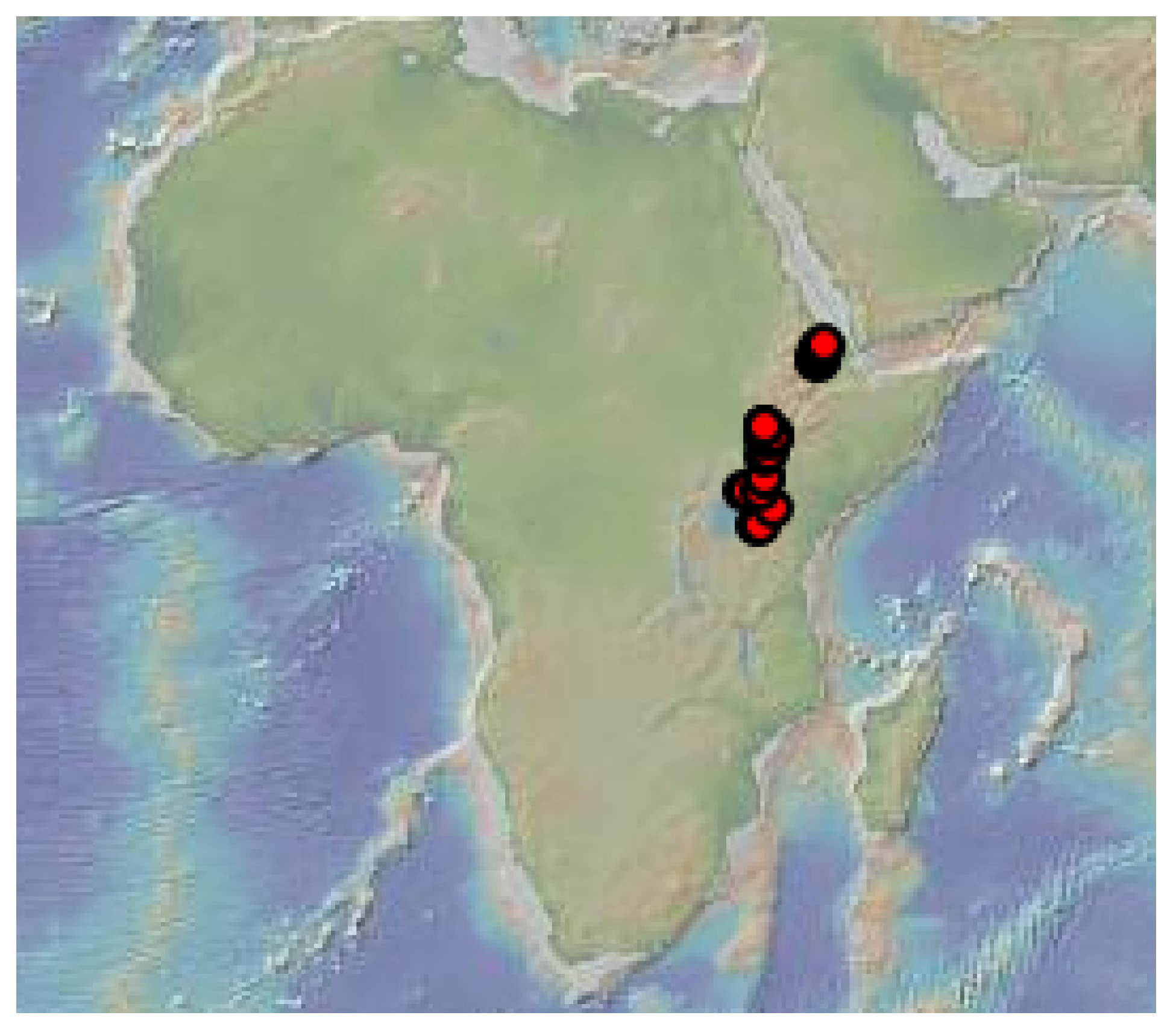
Figure 1. Soil carbonate stable isotope ( δ 13 C ) collected from various sites of East Africa [4].
Stats 02 00032 g001
Figure 2. East Africa soil-carbonate-stable isotope ( δ 13 C ) time series.
Stats 02 00032 g002
Figure 3. Frequency distribution of gaps of different lengths (red) and the number of not available observations (NAs) related to each gap (blue).
Stats 02 00032 g003
Figure 4. (A,B) Imputation by basic SSA and L 1 -SSA methods.
Stats 02 00032 g004
Figure 5. (AC) Imputation by interpolation methods.
Stats 02 00032 g005
Figure 6. (A,B) Imputation by the Kalman smoothing method.
Stats 02 00032 g006
Figure 7. (A,B) Imputation by LOCF and NOCB methods.
Stats 02 00032 g007
Figure 8. (AC) Imputation by weighted moving average methods.
Stats 02 00032 g008
Table 1. Summary statistics of the original and imputed time series.
Time SeriesMeanStandard DeviationMedianSkewnessKurtosis
Original−0.252.21−0.330.30−0.18
Basic SSA−0.432.10−0.630.45−0.15
L 1 -SSA−0.291.85−0.390.400.57
Linear Interpolation−0.232.34−0.370.32−0.49
Spline Interpolation−0.042.85−0.341.354.36
Stineman Interpolation−0.232.36−0.380.33−0.48
Kalman (ARIMA)−0.282.14−0.350.31−0.40
Kalman (StructTS)−0.352.09−0.620.38−0.34
LOCF−0.232.43−0.360.21−0.72
NOCB−0.242.51−0.480.47−0.32
SMA−0.292.19−0.340.30−0.42
LWMA−0.272.24−0.360.28−0.54
EWMA−0.262.32−0.380.28−0.64
Table 2. Mean squared errors (MSE) of different imputing methods.
ImputingPercent of Missing Values
Method10%20%30%40%
Basic SSA1.121.151.201.24
L 1 -SSA1.111.131.171.22
Linear Interpolation1.371.381.431.48
Spline Interpolation1.872.162.573.18
Stineman Interpolation1.391.431.481.56
Kalman (ARIMA)1.111.131.191.25
Kalman (StructTS)1.221.251.271.29
LOCF2.562.662.762.90
NOCB2.532.682.772.92
SMA1.211.241.271.33
LWMA1.181.211.251.31
EWMA1.231.261.311.38