Inferences About Two-Parameter Multicollinear Gaussian Linear Regression Models: An Empirical Type I Error and Power Comparison

Abstract

In linear regression analysis, the independence assumption is crucial and the ordinary least square (OLS) estimator generally regarded as the Best Linear Unbiased Estimator (BLUE) is applied. However, multicollinearity can complicate the estimation of the effect of individual variables, leading to potential inaccurate statistical inferences. Because of this issue, different types of two-parameter estimators have been explored. This paper compares t-tests for assessing the significance of regression coefficients, including several two-parameter estimators. We conduct a Monte Carlo study to evaluate these methods by examining their empirical type I error and power characteristics, based on established protocols. The simulation results indicate that some two-parameter estimators achieve better power gains while preserving the nominal size at 5%. Real-life data are analyzed to illustrate the findings of this paper.

1. Introduction

In linear regression analysis, the independence assumption of the explanatory variables is crucial, as the ordinary least square (OLS) estimator is commonly used as the Best Linear Unbiased Estimator (BLUE). However, multicollinearity presents a significant obstacle, complicating the estimation of unique effects for individual variables. This often leads to OLS producing inefficient and unreliable estimates, marked by high standard errors and inaccurate confidence intervals (Kibria, 2003) [1]. To overcome these challenges, researchers have developed various alternative biasing estimators to replace OLS, each with unique approaches to improve estimation accuracy. Pioneering efforts in this area include contributions from Hoerl and Kennard (1970) [2] and subsequent enhancements by Ehsanes Saleh and Kibria (1993) [3], Kibria (2003) [1], Alheety et al. (2025) [4], Dawoud and Kibria (2020) [5], Hoque and Kibria (2023) [6], Hoque and Kibria (2024) [7], Nayem et al. (2024) [8], and Yasmin and Kibria (2025) [9], among others.

Hypothesis testing is another aspect of statistical inference, especially in regression models, where it is necessary to test the significance of the coefficients. This procedure helps identify which variables are significant predictors of the outcome.

Our main objective is to find out the statistical significance of the regression coefficients within our model using hypothesis testing. However, the current body of research on this topic is somewhat limited. Halawa and Bassiouni (2000) [10] were instrumental in presenting approximate t-tests for regression coefficients within the framework of ridge regression, with a focus on empirical sizes and powers. Building on this, Cule et al. (2011) [11] assessed these tests for linear and logistic ridge regression frameworks, further advancing our understanding of their effectiveness across different types of regression models. Gokpinar and Ebegil (2016) [12] also contributed by evaluating the effectiveness of t-tests across various estimators of the ridge parameter $k$, based on insights from the existing literature. Additionally, Kibria and Banik (2019) [13] as well as Perez-Melo and Kibria (2020) [14] investigated the robustness of t-tests across different ridge parameters. Despite these advancements, continued research is essential to deepen our understanding and enhance methodologies for testing the significance of regression coefficients.

Additionally, within the context of the Liu estimator, Ullah et al. (2017) [15] focused on testing coefficients specific to this regression framework. Expanding on this work, Perez-Melo et al. (2022) [16] conducted a comparative analysis of Ridge, Liu, and Kibria Lukman estimators, enhancing our understanding of regression coefficient testing across different estimation methods. These studies underscore the significance of exploring diverse regression techniques and their implications for hypothesis testing in regression analysis.

This study aims to thoroughly contrast various t-test statistics for testing different regression coefficients across multiple two-parameter estimation methods. We will evaluate the performance of these tests within several frameworks, for example the Yang and Chang (2010) [17] estimator, Modified Ridge Type (MRT) estimator, and other two-parameter estimators, and compare them to ordinary least square (OLS). By employing Monte Carlo simulation, we will examine the empirical type I error for each and then estimate the power properties of each method, guided by procedures established by Halawa and Bassiouni (2000) [10] and Gokpinar and Ebegil (2016) [12]. We will look at different two-parameter estimators together to see which one performs better than others. Previous work has not comprehensively compared all two-parameter methods against OLS, so our objective is to examine most of them and recommend the ones that hold type I error rates and demonstrate gains in power. This research also seeks to enhance the understanding of regression coefficient testing methods and offer valuable insights for practitioners in model selection and interpretation in regression analysis.

This paper is structured as follows: Section 2 outlines the statistical methodology, detailing various estimators for different parameters $k$ and $d$. Section 3 presents the methods and explains the results of the simulation study. Section 4 provides an applied example to demonstrate the performance of several best selected methods compared to OLS. Finally, Section 5 offers a summary and concluding remarks.

2. Statistical Framework

In this section, we will explain the structure of the linear regression model and explore the estimators used in this context.

2.1. Framework of Model and Several Established Estimators

We consider the following model:

$$Y=X\beta +ϵ,ϵ~N\left(0,{\sigma }^2{I}_n\right),$$

(1)

where $Y$ is an $n\times 1$ vector representing a response variable, $X$ is an $n\times p$ regressor matrix, assumed to have a full rank, $\beta$ is a $p\times 1$ vector of regression coefficients, and $ϵ$ is an $n\times 1$ vector of normally distributed residuals, satisfying $E\left(ϵ\right)=0$ and $Var\left(ϵ\right)={\sigma }^2{I}_n$, with $I_n$ being an $n\times n$ identity matrix.

The ordinary least square (OLS) estimator of $\beta$ in the linear regression model is given by the following:

$${\widehat{\beta }}_{OLS}={\left(X^{T}X\right)}^{-1}{X}^{T}Y$$

(2)

To test whether the $i$th component of $\beta$ is equivalent to zero, i.e., $H_0:{\beta }_i=0 \mathrm{vs}. H_1:{\beta }_i\ne 0$, the test statistics is defined based on the OLS estimator:

$$t={\displaystyle \frac{{\widehat{\beta }}_i}{SE\left({\widehat{\beta }}_i\right)}},$$

(3)

where ${\widehat{\beta }}_i$ is the $i$th component of $\widehat{\beta }$, and $SE\left({\widehat{\beta }}_i\right)$ is the standard error of ${\widehat{\beta }}_i$, which is the square root of the $i$th diagonal entry of the covariance matrix $Var\left({\widehat{\beta }}_{OLS}\right)={\sigma }^2{\left(X^{T}X\right)}^{-1}$, where

$$\widehat{{\sigma }^2}={\displaystyle \frac{{\left(Y-X{\widehat{\beta }}_{OLS}\right)}^T\left(Y-X{\widehat{\beta }}_{OLS}\right)}{n-p-1}}.$$

(4)

The test statistic in Equation (3) follows Student’s t-distribution with $n-p-1$ degrees of freedom under the null hypothesis. However, if $X^{T}X$ becomes ill conditioned when multicollinearity arises, the OLS estimator may yield unbalanced estimates with excessively high variances. To mitigate this issue, Hoerl and Kennard (1970) [2] established other shrinkage regression estimators.

2.2. Two Parameter Estimators

In this section, we will consider various two-parameter estimators that are available in the literature.

2.2.1. Liu Type of Two-Parameter Estimator

To overcome the multicollinearity problem, Liu (2003) [18] proposed a two-parameter estimator,

$${\widehat{\beta }}_{LTE}={\left(X^{T}X+kI\right)}^{-1}\left(X^{T}Y-d{\beta }^{\mathrm{*}}\right),$$

(5)

where ${\beta }^{*}$ is any estimator of $\beta$; if we choose ${\beta }^{*}={\widehat{\beta }}_{OLS}$ and then we can obtain

$${\widehat{\beta }}_{LTE}={\left(X^{T}X+kI\right)}^{-1}\left(X^{T}X-dI\right){\widehat{\beta }}_{OLS}.$$

The expected value and covariance matrix are given, respectively, as follows:

$$E\left({\widehat{\beta }}_{LTE}\right)=A_{LTE}\beta \mathrm{and}$$

$$Var\left({\widehat{\beta }}_{LTE}\right)={{\sigma }_{LTE}^2{A}_{LTE}\left(X^{T}X\right)}^{-1}{A}_{LTE}^T$$

where $A_{LTE}={\left(X^{T}X+kI\right)}^{-1}\left(X^{T}X-dI\right)$, and ${\sigma }_{LTE}^2$ is estimated as follows:

$${\widehat{{\sigma }^2}}_{LTE}={\displaystyle \frac{{\left(Y-X{\widehat{\beta }}_{LTE}\right)}^T(Y-X{\widehat{\beta }}_{LTE})}{n-p-1}}$$

(6)

From Liu (2003) [18], we will consider the following values of $k$ and $d$:

$$\widehat{\mathrm{k}}={\displaystyle \frac{{\lambda }_1-100\ast {\lambda }_p}{99}} \mathrm{a}\mathrm{n}\mathrm{d} \widehat{\mathrm{d}}={\displaystyle \frac{{\sum }_{j=1}^p\left(\frac{\left({\widehat{\sigma }}^2-k{\alpha }_j^2\right)}{{\left({\lambda }_j+\widehat{k}\right)}^2}\right)}{{\sum }_{j=1}^p\left(\frac{\left({\widehat{\sigma }}^2+{\lambda }_j{\widehat{\alpha }}_j^2\right)}{{{\lambda }_j\left({\lambda }_j+\mathrm{k}\right)}^2}\right)}}.$$

2.2.2. Ozkale and Kaciranlar Two-Parameter Estimator

Ozkale and Kaciranlar (2007) [19] consider the following estimator,

$${\widehat{\beta }}_{TP}=A_{TP}{\widehat{\beta }}_{OLS},$$

(7)

where $A_{TP}={\left(X^{T}X+kI\right)}^{-1}\left(X^{T}X+kdI\right)$.

We have the expected value and covariance matrix for ${\widehat{\beta }}_{TP}$ as follows:

$$\begin{array}{l}E\left({\widehat{\beta }}_{TP}\right)=A_{TP}\beta \mathrm{a}\mathrm{n}\mathrm{d}\\ Var\left({\widehat{\beta }}_{TP}\right)={\sigma }_{TP}^2{A}_{TP}{\left(X^{T}X\right)}^{-1}{A}_{TP}^T,\end{array}$$

${\sigma }_{TP}^2$ is estimated as follows:

$${\widehat{{\sigma }^2}}_{TP}={\displaystyle \frac{{\left(Y-X{\widehat{\beta }}_{TP}\right)}^T(Y-X{\widehat{\beta }}_{TP})}{n-p-1}}$$

(8)

Following Ozkale and Kaciranlar (2007) [19], we have the optimal $d$ and $k$ as follows:

$${\widehat{d}}_{opt}={\displaystyle \frac{{\sum }_{j=1}^p\frac{(k{\widehat{\alpha }}_j^2-{\widehat{\sigma }}^2)}{{\left({\lambda }_j+k\right)}^2}}{{\sum }_{j=1}^p\frac{k({\widehat{\sigma }}^2+{\widehat{\mathsf{\alpha }}}_{\mathrm{j}}{\lambda }_j)}{{\lambda }_j{\left({\lambda }_j+k\right)}^2}}},$$

and

$${\widehat{\mathrm{k}}}_{\mathrm{j}}={\displaystyle \frac{{\widehat{\sigma }}^2}{{\widehat{\alpha }}_j^2-d\left(\frac{{\widehat{\sigma }}^2}{{\lambda }_j}+{\widehat{\alpha }}_j^2\right)}}.$$

Hoerl et al. (1975) [20] used the harmonic mean of $k$ values which is identified by Hoerl and Kennard (1970) [2]. Also, Kibria (2003) [1] proposed the arithmetic mean of the same $k$ values. Therefore, both arithmetic and harmonic means of $k$ values can be used for estimating this shrinkage parameter $k$. Then,

$${\widehat{k}}_{HM}={\displaystyle \frac{p{\widehat{\sigma }}^2}{{\sum }_{j=1}^p\left[{\widehat{\alpha }}_j^2-d\left(\frac{{\widehat{\sigma }}^2}{{\lambda }_j}+{\alpha }_j^2\right)\right]}} \mathrm{and} {\widehat{k}}_{AM}={\displaystyle \frac{1}{p}}{\sum }_{j=1}^p{\displaystyle \frac{{\widehat{\sigma }}^2}{{\widehat{\alpha }}_j^2-d\left(\frac{{\widehat{\sigma }}^2}{{\lambda }_j}+{\alpha }_j^2\right)}}.$$

We can see that ${\widehat{d}}_{opt}$ depends on k and $\widehat{k}$ also depends on $d$. So, we can select parameters $d$ and $k$ by applying the following iterative method.

Step 1. First, we will calculate $\widehat{d}=\min \left[{\displaystyle \frac{{\widehat{\alpha }}_j^2}{\frac{{\widehat{\sigma }}^2}{{\lambda }_j}+{\widehat{\alpha }}_j^2}}\right]$.

Step 2. Then, we will obtain ${\widehat{k}}_{AM}$ or ${\widehat{k}}_{HM}$ by using $\widehat{d}$ from Step 1.

Step 3. We will estimate ${\widehat{d}}_{opt}$ from estimators ${\widehat{k}}_{AM}$ or ${\widehat{k}}_{HM}$ from Step 2.

Step 4. If we find that ${\widehat{d}}_{opt}$ is negative, we need to use ${\widehat{d}}_{opt}=\widehat{d}$ because $\widehat{d}$ is always less than one and bigger than zero, i.e., $0<\widehat{d}<1$.

2.2.3. New Biased Estimator Based on Ridge

Sakallıoglu˘ and Kiciranlar (2008) [21] proposed the following two-parameter estimator:

$$\begin{array}{c}{\widehat{\beta }}_{NBE}={\left(X^{T}X+I\right)}^{-1}\left(X^{T}y+d{\widehat{\beta }}_{Ridge}\right)\\ ={\left(X^{T}X+I\right)}^{-1}\left(X^{T}X+\left(d+k\right)I\right){\left(X^{T}X+kI\right)}^{-1}{X}^{T}X{\widehat{\beta }}_{OLS}\end{array}$$

(9)

The expected value and covariance matrix are given, respectively, as

$$E\left({\widehat{\beta }}_{NBE}\right)=A_{NBE}\beta \mathrm{and}$$

$$Var\left({\widehat{\beta }}_{NBE}\right)={{\sigma }_{NBE}^2{A}_{NBE}\left(X^{T}X\right)}^{-1}{A}_{NBE}^T,$$

where $A_{NBE}={\left(X^{T}X+I\right)}^{-1}\left(X^{T}X+\left(d+k\right)I\right){\left(X^{T}X+kI\right)}^{-1}{X}^{T}X,$ and ${\sigma }_{NBE}^2$ is estimated as

$${\widehat{{\sigma }^2}}_{NBE}={\displaystyle \frac{{\left(Y-X{\widehat{\beta }}_{NBE}\right)}^T(Y-X{\widehat{\beta }}_{NBE})}{n-p-1}}.$$

(10)

For estimating the unknown parameters $k$ and $d$, we can choose

$${\widehat{d}}_{opt}={\displaystyle \frac{{\sum }_{j=1}^p\frac{{\lambda }_j({\widehat{\alpha }}_j^2-{\widehat{\sigma }}^2)}{{\left({\lambda }_j+1\right)}^2({\lambda }_j+k)}}{{\sum }_{j=1}^p\frac{{\lambda }_j({\lambda }_j{\widehat{\alpha }}_j^2+{\widehat{\sigma }}^2)}{{\left({\lambda }_j+1\right)}^2{\left({\lambda }_j+k\right)}^2}}},$$

where for fixed $k$, we use $k_{HK}={\displaystyle \frac{{\widehat{\sigma }}^2}{{\sum }_{j=1}^p{\widehat{\alpha }}_j^2}}$ and $k_{HKB}={\displaystyle \frac{p{\widehat{\sigma }}^2}{{\sum }_{j=1}^p{\widehat{\alpha }}_j^2}}$.

2.2.4. Yang and Chang Two-Parameter Estimator

Yang and Chang (2010) [17] consider the following estimator:

$${\widehat{\beta }}_{YC}=Y_{k,d}{\widehat{\beta }}_{OLS}$$

(11)

where $Y_{k,d}={\left(X^{T}X+I\right)}^{-1}\left(X^{T}X+dI\right){\left(X^{T}X+kI\right)}^{-1}\left(X^{T}X\right)$, and $k$ and $d$ are biasing parameters.

The expected value and covariance matrix of ${\widehat{\beta }}_{YC}$ are as follows:

$$\begin{gathered} E\left({\widehat{\beta }}_{YC}\right)=Y_{k,d}\beta , \\ Var\left({\widehat{\beta }}_{YC}\right)={{\sigma }_{YC}^{2}Y}_{k,d}{\left(X^{T}X\right)}^{-1}{Y}_{k,d}^T \end{gathered}$$

and ${\sigma }_{YC}^2$ is estimated as

$${\widehat{{\sigma }^2}}_{YC}={\displaystyle \frac{{\left(Y-X{\widehat{\beta }}_{YC}\right)}^T(Y-X{\widehat{\beta }}_{YC})}{n-p-1}}.$$

(12)

For $k$, we fix $d$, and based on Yang and Chang (2010) [17], we obtain the optimal $k$ as

$${\widehat{\mathrm{k}}}_{\mathrm{j}}={\displaystyle \frac{{\widehat{\sigma }}^2\left({\lambda }_j+d\right)-\left(1-d\right){\lambda }_j{\widehat{\alpha }}_j^2}{\left({\lambda }_j+1\right){\widehat{\alpha }}_j^2}}.$$

We apply different formulas for this parameter, such as arithmetic mean, harmonic mean, and median.

Then, we obtain

$${\widehat{d}}_{opt}={\displaystyle \frac{{\sum }_{i=1}^p\left[\left(\left(k+1\right){\lambda }_j+k\right){\lambda }_j{\widehat{\alpha }}_j^2-{\lambda }_j^2{\widehat{\sigma }}^2\right]/\left[{\left({\lambda }_j+1\right)}^2{\left({\lambda }_j+k\right)}^2\right]}{{\sum }_{i=1}^p\left({\widehat{\sigma }}^2+{\lambda }_j{\widehat{\alpha }}_j^2\right){\lambda }_j/\left[{\left({\lambda }_j+1\right)}^2\left({\left({\lambda }_j+k\right)}^2\right)\right]}}.$$

The estimators of parameters $k$ and $d$ in ${\widehat{\beta }}_{YC}$ are acquired by using the following iterative method:

Step 1: Obtain an initial estimate using $\widehat{d}=\min \left({\displaystyle \frac{{\widehat{\sigma }}^2}{{\widehat{\alpha }}_j^2}}\right)$.

Step 2: Estimate $\widehat{k}$ using $\widehat{d}$ in Step 1.

Step 3: Find ${\widehat{d}}_{opt}$ using $\widehat{k}$ in Step 2.

Step 4. If $0<{\widehat{d}}_{opt}<1$ does not hold, use ${\widehat{d}}_{opt}=\widehat{d}$.

2.2.5. Almost Unbiased Two-Parameter Estimator

Wu and Yang (2011) [22] consider the following estimator:

$${\widehat{\beta }}_{AUTP}=[I-k^2{\left(1-d\right)}^2{\left(X^{T}X+kI\right)}^{-2}]{\widehat{\beta }}_{OLS}$$

(13)

The expected value and covariance matrix of ${\widehat{\beta }}_{AUTP}$ are as follows:

$$\begin{array}{l}E\left({\widehat{\beta }}_{AUTP}\right)=A_{AUTP}\beta ,\\ Var\left({\widehat{\beta }}_{AUTP}\right)={{\sigma }_{AUTP}^{2}A}_{AUTP}{\left(X^{T}X\right)}^{-1}{A}_{AUTP}^T,\end{array}$$

where $A_{AUTP}=[I-k^2{\left(1-d\right)}^2{\left(X^{T}X+kI\right)}^{-2}]$ and ${\sigma }_{AUTP}^2$ is estimated as

$${\widehat{{\sigma }^2}}_{AUTP}={\displaystyle \frac{{\left(Y-X{\widehat{\beta }}_{AUTP}\right)}^T(Y-X{\widehat{\beta }}_{AUTP})}{n-p-1}}.$$

(14)

Now, $d_j=1-{\displaystyle \frac{\left({\lambda }_j+k\right)\widehat{\sigma }}{k}}{\left({\displaystyle \frac{1}{{\sigma }^2+{\lambda }_j{\widehat{\alpha }}_j^2}}\right)}^{{\displaystyle \frac{1}{2}}}$ and $k_j={\displaystyle \frac{\widehat{\sigma }{\lambda }_j}{\left(1-d\right)\sqrt{{\widehat{\sigma }}^2+{\lambda }_j{\widehat{\alpha }}_j^2}-\widehat{\sigma }}}$.

We apply the arithmetic mean and harmonic mean for this parameter.

We can select parameters $k$ and $d$ by using the following approach.

Step 1: We compute $\widehat{d}$ using $d=1-\min \left({\displaystyle \frac{\widehat{\sigma }}{\sqrt{{\lambda }_j{\widehat{\alpha }}_j^2+{\widehat{\sigma }}^2}}}\right)$.

Step 2: We obtain ${\widehat{k}}_j$ using $\widehat{d}$.

Step 3: We find ${\widehat{d}}_j$ using ${\widehat{k}}_j$ from Step 2.

Step 4. If ${\widehat{d}}_j$ is negative, we need ${\widehat{d}}_j=\widehat{d}$ because it is always less than 1 but it may be smaller than 0.

2.2.6. Unbiased Two-Parameter Estimator

Wu (2014) [23] considers the following two-parameter estimator:

$${\widehat{\beta }}_{UTP}=A_{UTP}{\widehat{\beta }}_{OLS}+(1-A_{UTP})J$$

(15)

where $A_{UTP}={\left(X^{T}X+kI\right)}^{-1}(X^{T}X+kdI)$ and $J~N\left(\beta ,\left({\displaystyle \frac{{\sigma }^2}{k\left(1-d\right)}}\right)\left(X^{T}X+kdI\right)X^T{X}^{-1}\right)$ for $k>0$, $0<d<1$, and $J$ is called the prior information and is a random vector which has a specified mean and covariance.

The expected value and covariance matrix of ${\widehat{\beta }}_{UTP}$ are as follows:

$$\begin{array}{l}E\left({\widehat{\beta }}_{UTP}\right)=\beta ,\\ Var\left({\widehat{\beta }}_{UTP}\right)={{\sigma }_{UTP}^{2}A}_{UTP}{\left(X^{T}X\right)}^{-1},\end{array}$$

and ${\sigma }_{UTP}^2$ is estimated as

$${\widehat{{\sigma }^2}}_{UTP}={\displaystyle \frac{{\left(Y-X{\widehat{\beta }}_{UTP}\right)}^T(Y-X{\widehat{\beta }}_{UTP})}{n-p-1}}.$$

(16)

Now, for fixed $k$, we need to obtain an estimator of $d$ as follows:

$$\widehat{d}=1-{\displaystyle \frac{{\widehat{\sigma }}^2[p+ktr{\left(X^{T}X\right)}^{-1}]}{k\left({\widehat{\beta }}_{OLS}-J\right){\left({\widehat{\beta }}_{OLS}-J\right)}^T}}$$

where $tr{\left(X^{T}X\right)}^{-1}={\sum }_{j=1}^{p}1/{\lambda }_j$.

If $k\left({\widehat{\beta }}_{OLS}-J\right){\left({\widehat{\beta }}_{OLS}-J\right)}^T-{\widehat{\sigma }}^2\left[p+ktr{\left(X^{T}X\right)}^{-1}\right]>0,$ then

$${\widehat{d}}^{\mathrm{*}}=1-{\displaystyle \frac{{\widehat{\sigma }}^2\left[p+ktr{\left(X^{T}X\right)}^{-1}\right]}{k\left({\widehat{\beta }}_{OLS}-J\right){\left({\widehat{\beta }}_{OLS}-J\right)}^T}};$$

Otherwise, ${\widehat{d}}^{\mathrm{*}}=1$.

Parameter $k$ is defined as

$$\widehat{k}={\displaystyle \frac{{p\widehat{\sigma }}^2}{\left(1-d\right)\left({\widehat{\beta }}_{OLS}-J\right){\left({\widehat{\beta }}_{OLS}-J\right)}^T-{\sigma }^{2}tr{\left(X^{T}X\right)}^{-1}}}.$$

If $\left(1-d\right)\left({\widehat{\beta }}_{OLS}-J\right){\left({\widehat{\beta }}_{OLS}-J\right)}^T-{\widehat{\sigma }}^{2}tr{\left(X^{T}X\right)}^{-1}>0$, then

$${\widehat{k}}^{\mathrm{*}}={\displaystyle \frac{{p\sigma }^2}{\left(1-d\right)\left({\widehat{\beta }}_{OLS}-J\right){\left({\widehat{\beta }}_{OLS}-J\right)}^T-{\widehat{\sigma }}^{2}tr{\left(X^{T}X\right)}^{-1}}};$$

Otherwise,

$${\widehat{k}}^{\mathrm{*}}={\displaystyle \frac{{p\widehat{\sigma }}^2}{\left(1-d\right)\left({\widehat{\beta }}_{OLS}-J\right){\left({\widehat{\beta }}_{OLS}-J\right)}^T}}.$$

The selection of parameters $k$ and $d$ can be obtained by using the following approach.

Step 1: Estimate $\widehat{d}=\min \left({\displaystyle \frac{{\widehat{\sigma }}^2}{{\widehat{\alpha }}_j^2}}\right)$.

Step 2: Compute a random vector J.

Step 3: Compute $\widehat{k}$ using J and $\widehat{d}$.

Step 4: Compute $\widehat{d}$.

2.2.7. Dorugade Modified Two-Parameter Estimator

Dorugade (2014) [24] considers the following modified estimator:

$${\widehat{\beta }}_{MTP}=A_{MTP}{\widehat{\beta }}_{OLS}$$

(17)

where $A_{MTP}=\left[I+k\left(1-d\right){\left(X^{T}X+kdI\right)}^{-1}\right][I-kd{\left(X^{T}X+kdI\right)}^{-1}]$.

The expected value and covariance matrix of ${\widehat{\beta }}_{MTP}$ are as follows:

$$\begin{array}{l}E\left({\widehat{\beta }}_{MTP}\right)=A_{MTP}\beta ,\\ Var\left({\widehat{\beta }}_{MTP}\right)={{\sigma }_{MTP}^{2}A}_{MTP}{\left(X^{T}X\right)}^{-1}{A}_{MTP}^T,\end{array}$$

and ${\sigma }_{MTP}^2$ is estimated as

$${\widehat{{\sigma }^2}}_{MTP}={\displaystyle \frac{{\left(Y-X{\widehat{\beta }}_{MTP}\right)}^T(Y-X{\widehat{\beta }}_{MTP})}{n-p-1}}.$$

(18)

For unknow values of $k$ and $d$, some well know methods are ${\widehat{k}}_1={\displaystyle \frac{p{\widehat{\sigma }}^2}{{\sum }_{j=1}^p{\widehat{\alpha }}_j^2}}$ and ${\widehat{k}}_2=median\left({\displaystyle \frac{{\widehat{\sigma }}^2}{{\widehat{\alpha }}_j^2}}\right)$.

The optimal $d$ can be considered as follows:

$${\widehat{d}}_{opt}=\sum _{j=1}^p{\displaystyle \frac{\left({\lambda }_j+k\right)\left({{{\widehat{\sigma }}^2+\lambda }_j\widehat{\alpha }}_j^2\right)-{\lambda }_j}{k{\widehat{\alpha }}_j^2}}$$

2.2.8. Modified Almost Unbiased Liu Estimator

Arumairajan and Wijekoon (2017) [25] consider the following two-parameter estimator:

$${\widehat{\beta }}_{MAULE}=A_{MAULE}{\widehat{\beta }}_{OLS}$$

(19)

where $A_{MAULE}=\left(1-{\left(1-d\right)}^2{\left(X^{T}X+I\right)}^{-2}\right){\left(X^{T}X+kI\right)}^{-1}{X}^{T}X$.

The expected value and covariance matrix of ${\widehat{\beta }}_{MAULE}$ are as follows:

$$\begin{array}{l}E\left({\widehat{\beta }}_{MAULE}\right)=A_{MAULE}\beta ,\\ Var\left({\widehat{\beta }}_{MAULE}\right)={{\sigma }_{MAULE}^{2}A}_{MAULE}{\left(X^{T}X\right)}^{-1}{A}_{MAULE}^T,\end{array}$$

and ${\sigma }_{MAULE}^2$ is estimated as

$${\widehat{{\sigma }^2}}_{MAULE}={\displaystyle \frac{{\left(Y-X{\widehat{\beta }}_{MAULE}\right)}^T(Y-X{\widehat{\beta }}_{MAULE})}{n-p-1}}.$$

(20)

Now, ${\widehat{d}}_{opt}=1-\sqrt{{\displaystyle \frac{{\sum }_{j=1}^p\frac{{\lambda }_j\left({\widehat{\sigma }}^2-k{\widehat{\alpha }}_j^2\right)}{{\left({\lambda }_j+k\right)}^2{\left({\lambda }_j+1\right)}^2}}{{\sum }_{j=1}^p\frac{{\lambda }_j\left({\widehat{\sigma }}^2+{\lambda }_j{\widehat{\alpha }}_j^2\right)}{{\left({\lambda }_j+1\right)}^4{\left({\lambda }_j+k\right)}^2}}}}$, and ${\widehat{k}}_j={\displaystyle \frac{{\widehat{\sigma }}^2{\left({\lambda }_j+1\right)}^2{\lambda }_j-{\left(1-d\right)}^2{\lambda }_j({\widehat{\sigma }}^2+{\widehat{\alpha }}_j^2)}{{\widehat{\alpha }}_j^2{\left({\lambda }_j+1\right)}^2}}$.

For the optimal value, we use the arithmetic mean value of $k$.

2.2.9. Modified Almost Unbiased Two-Parameter Estimator

Lukman et al. (2019) [26] consider the following estimator:

$${\widehat{\beta }}_{MAUTP}=A_{MAUTP}{\widehat{\beta }}_{OLS}$$

(21)

where $A_{MAUTP}=\left(I-k^2{\left(1-d\right)}^2{\left(X^{T}X+kI\right)}^{-2}\right){\left(X^{T}X+kI\right)}^{-1}{X}^{T}X$.

The expected value and covariance matrix of ${\widehat{\beta }}_{MAUTP}$ are as follows:

$$\begin{array}{c}E\left({\widehat{\beta }}_{MAUTP}\right)=A_{MAUTP}\beta ,\\ Var\left({\widehat{\beta }}_{MAUTP}\right)={{\sigma }_{MAUTP}^{2}A}_{MAUTP}{\left(X^{T}X\right)}^{-1}{A}_{MAUTp}^T,\end{array}$$

and ${\sigma }_{MAUTP}^2$ is estimated as

$${\widehat{{\sigma }^2}}_{MAUTP}={\displaystyle \frac{{\left(Y-X{\widehat{\beta }}_{MAUTP}\right)}^T(Y-X{\widehat{\beta }}_{MAUTP})}{n-p-1}}.$$

(22)

For the estimation of $k$ and $d$, following Hoerl and Kennard (1970) [2], $\widehat{k}={\displaystyle \frac{{\widehat{\sigma }}^2}{{\widehat{\alpha }}_j^2}}$, and the harmonic version of the proposed $\widehat{k}$ is ${\widehat{k}}_{HMP}={\displaystyle \frac{p{\widehat{\sigma }}^2}{{\sum }_{j=1}^p{\widehat{\alpha }}_j^2}}$, and ${\widehat{\mathrm{d}}}_{\mathrm{o}\mathrm{p}\mathrm{t}}=\min \left({\displaystyle \frac{{\widehat{\alpha }}_j^2}{\frac{{\widehat{\sigma }}^2}{{\widehat{\alpha }}_j^2}+{\widehat{\alpha }}_j^2}}\right)$.

2.2.10. Modified New Two-Parameter Estimator

Lukman et al. (2019) [27] consider the following estimator:

$${\widehat{\beta }}_{MNTP}={\left(X^{T}X+kI\right)}^{-1}[\left(X^{T}X+kdI\right){\widehat{\beta }}_{OLS}+k\left(1-d\right)b]$$

(23)

where $b$ is the prior information on $\beta$ and it tends to become $b$ if $k$ approaches infinity.

Let us recall that $k\left(1-d\right)=\left(X^{T}X+kI\right)-\left(X^{T}X+kdI\right)$ and let $A_{MNTP}={\left(X^{T}X+kI\right)}^{-1}\left(X^{T}X+kdI\right)$.

The expected value and covariance matrix of ${\widehat{\beta }}_{MNTP}$ are as follows:

$$\begin{array}{c}E\left({\widehat{\beta }}_{MNTP}\right)=A_{MNTP}\beta +(I-A_{MNTP})b,\\ Var\left({\widehat{\beta }}_{MNTP}\right)={{\sigma }_{MNTP}^{2}A}_{MNTP}{\left(X^{T}X\right)}^{-1}{A}_{MNTP}^T,\end{array}$$

and ${\sigma }_{MNTP}^2$ is estimated as

$${\widehat{{\sigma }^2}}_{MNTP}={\displaystyle \frac{{\left(Y-X{\widehat{\beta }}_{MNTP}\right)}^T(Y-X{\widehat{\beta }}_{MNTP})}{n-p-1}}.$$

(24)

For $k$, we fix $d$, based on Lukman et al. (2019) [27], and we obtain the optimal $k$ as

$${\widehat{k}}_j={\displaystyle \frac{{\widehat{\sigma }}^2{\lambda }_j}{{\lambda }_j{\left({\widehat{\alpha }}_j-b\right)}^2-\widehat{d}({\lambda }_j{\left({\widehat{\alpha }}_j-b\right)}^2+{\widehat{\sigma }}^2)}},$$

and the harmonic mean is

$${\widehat{k}}_{HMP}={\displaystyle \frac{p}{{\sum }_{j=1}^{p}1/{\widehat{\mathrm{k}}}_{\mathrm{j}}}}.$$

Then, we obtain

$${\widehat{d}}_{opt}={\displaystyle \frac{{\sum }_{j=1}^p\left[\left(\mathrm{k}{\lambda }_j{\left({\widehat{\alpha }}_j-b\right)}^2\right)-{\widehat{\sigma }}^2{\lambda }_j\right]}{{\sum }_{j=1}^p\left({\widehat{\sigma }}^2\widehat{k}+k{\lambda }_j{\left({\widehat{\alpha }}_j-b\right)}^2\right)}}.$$

The selection of parameters $k$ and $d$ in ${\widehat{\beta }}_{MNTP}$ is obtained using the following method:

Step 1: First, we will obtain an initial estimate of $d$ using $\widehat{d}=\min \left({\displaystyle \frac{{\lambda }_j{\left({\widehat{\alpha }}_j-b\right)}^2}{{\lambda }_j{\left({\widehat{\alpha }}_j-b\right)}^2+{\widehat{\sigma }}^2}}\right)$.

Step 2: We will obtain $\widehat{k}$ using $\widehat{d}$.

Step 3: We will estimate ${\widehat{d}}_{opt}$ using $\widehat{k}$.

Step 4. If ${\widehat{d}}_{opt}$ is negative, we must use ${\widehat{d}}_{opt}=\widehat{d}$. However, $\widehat{d}$ takes a value between 0 and 1.

2.2.11. Modified Ridge Type

Lukman et al. (2019) [28] consider the following two-parameter estimator:

$${\widehat{\beta }}_{MRT}=M_{k,d}{\widehat{\beta }}_{OLS}$$

(25)

where $M_{k,d}={\left(X^{T}X+k\left(1+d\right)I\right)}^{-1}\left(X^{T}X\right)$, with $k$ and $d$ as biasing parameters.

The expected value and covariance matrix of ${\widehat{\beta }}_{MRT}$ are as follows:

$$\begin{array}{c}E\left({\widehat{\beta }}_{MRT}\right)=M_{k,d}\beta ,\\ Var\left({\widehat{\beta }}_{MRT}\right)={\sigma }_{MRT}^2{M}_{k,d}{\left(X^{T}X\right)}^{-1}{M}_{k,d}^T,\end{array}$$

and ${\sigma }_{MRT}^2$ is estimated as

$${\widehat{{\sigma }^2}}_{MRT}={\displaystyle \frac{{\left(Y-X{\widehat{\beta }}_{MRT}\right)}^T(Y-X{\widehat{\beta }}_{MRT})}{n-p-1}}.$$

(26)

As the shrinkage parameters $k$ and $d$ are both unknown, it is necessary to estimate them from the observed data. This section provides the formulas for various shrinkage parameter regression estimators.

Lukman et al. (2019) [28] proposed an estimator as follows:

$${\widehat{\mathrm{k}}}_{\mathrm{j}}={\displaystyle \frac{{\widehat{\sigma }}^2}{\left(1+d\right){\widehat{\alpha }}_j^2}}.$$

We can obtain the harmonic mean of ${\widehat{k}}_j$ as

$${\widehat{k}}_{HMP}={\displaystyle \frac{p{\widehat{\sigma }}^2}{{\sum }_{j=1}^p\left(1+d\right){\widehat{\alpha }}_j^2}},$$

and

$${\widehat{\mathrm{d}}}_{\mathrm{j}}={\displaystyle \frac{{\widehat{\sigma }}^2}{k{\widehat{\alpha }}_j^2}}-1.$$

Also, the harmonic means of ${\widehat{d}}_j$ is

$${\widehat{d}}_{MRT}={\displaystyle \frac{p}{{\sum }_{j=1}^p\left(\frac{1}{{\widehat{\mathrm{d}}}_{\mathrm{j}}}\right)}}.$$

The selection of parameters $k$ and $d$ in ${\widehat{\beta }}_{MRT}$ is obtained by using the following method:

Step 1: We need to obtain an initial estimate of $d$ using $\widehat{d}=\min \left({\displaystyle \frac{{\widehat{\sigma }}^2}{{\widehat{\alpha }}_j^2}}\right)$.

Step 2: We obtain ${\widehat{k}}_{HMP}$ using $\widehat{d}$ from Step 1.

Step 3: We estimate ${\widehat{d}}_{MRT}$ using ${\widehat{k}}_{HMP}$ from Step 2.

Step 4. If ${\widehat{d}}_{opt}$ is negative, we use ${\widehat{d}}_{MRT}=\widehat{d}$.

2.2.12. A New Biased Estimator by Dawoud and Kibria

Dawoud and Kibria (2020) [5] consider the following two-parameter estimator:

$${\widehat{\beta }}_{DK}=A_{DK}{\widehat{\beta }}_{OLS}$$

(27)

where $A_{DK}={\left(X^{T}X+k\left(1+d\right)I\right)}^{-1}\left(X^{T}X-k\left(1+d\right)I\right)$.

The expected value and covariance matrix of ${\widehat{\beta }}_{DK}$ are as follows:

$$\begin{array}{c}E\left({\widehat{\beta }}_{DK}\right)=A_{DK}\beta ,\\ Var\left({\widehat{\beta }}_{DK}\right)={{\sigma }_{DK}^{2}A}_{DK}{\left(X^{T}X\right)}^{-1}{A}_{DK}^T,\end{array}$$

and ${\sigma }_{DK}^2$ is estimated as

$${\widehat{{\sigma }^2}}_{DK}={\displaystyle \frac{{\left(Y-X{\widehat{\beta }}_{DK}\right)}^T(Y-X{\widehat{\beta }}_{DK})}{n-p-1}}.$$

(28)

For $k$, we fix $d$, and we obtain the optimal $k$ as

$${\widehat{\mathrm{k}}}_{\mathrm{j}}={\displaystyle \frac{{\widehat{\sigma }}^2}{\left(1+\mathrm{d}\right)\left(\frac{{\widehat{\sigma }}^2}{{\lambda }_j}+2{\widehat{\alpha }}_j^2\right)}},$$

where $k_{min}=\mathrm{m}\mathrm{i}\mathrm{n} \left({\widehat{k}}_{^j}\right)$.

Then, for the optimal $d$, we obtain

$${\widehat{d}}_j={\displaystyle \frac{{\widehat{\sigma }}^2{\lambda }_j}{m}}-1,$$

where $m=\mathrm{k}({\widehat{\sigma }}^2+2{\lambda }_j{\widehat{\alpha }}_j^2)$.

In addition, $d_{min}=\mathrm{m}\mathrm{i}\mathrm{n} \left({\widehat{d}}_{^j}\right)$.

The selection of parameters $k$ and $d$ in ${\widehat{\beta }}_{DK}$ is obtained by using the following method:

Step 1: Obtain an initial estimate of $d$ using $\widehat{d}=\min \left({\displaystyle \frac{{\widehat{\sigma }}^2}{{\widehat{\alpha }}_j^2}}\right)$.

Step 2: Obtain $\widehat{k}$ using $\widehat{d}$.

Step 3: Estimate ${\widehat{d}}_{min}$ using $\widehat{k}$.

Step 4. If ${\widehat{d}}_{opt}$ is not between 0 and 1, use ${\widehat{d}}_{min}=\widehat{d}$.

2.2.13. Generalized Two-Parameter Estimator

Zeinal (2020) [29] proposed the following two-parameter estimator:

$${\widehat{\beta }}_{GTP}={\left(X^{T}X+kI\right)}^{-1}\left(X^{T}X+kD\right){\widehat{\beta }}_{OLS}$$

(29)

where $D=diag(d_1,d_2,\dots ,d_p)$.

The expected value and covariance matrix of ${\widehat{\beta }}_{GTP}$ are as follows:

$$\begin{array}{l}E\left({\widehat{\beta }}_{GTP}\right)=A_{GTP}\beta ,\\ Var\left({\widehat{\beta }}_{GTP}\right)={\sigma }_{GTP}^2{A}_{GTP}{\left(X^{T}X\right)}^{-1}{A}_{GTP}^T,\end{array}$$

where $A_{GTP}={\left(X^{T}X+kI\right)}^{-1}\left(X^{T}X+kD\right)$.

and ${\sigma }_{GTP}^2$ is estimated as

$${\widehat{{\sigma }^2}}_{GTP}={\displaystyle \frac{{\left(Y-X{\widehat{\beta }}_{GTP}\right)}^T(Y-X{\widehat{\beta }}_{GTP})}{n-p-1}}.$$

(30)

For the unknown parameter, we obtain the optimal $d_j$ for fixed $k$ as

$${\widehat{d}}_j={\displaystyle \frac{(k{\widehat{\alpha }}_j^2-{\widehat{\sigma }}^2){\lambda }_j}{k({\widehat{\sigma }}^2+{\widehat{\alpha }}_j^2{\lambda }_j)}}.$$

Then, we obtain

$${\widehat{k}}_j={\displaystyle \frac{{\widehat{\sigma }}^2}{{\widehat{\alpha }}_j^2-d_j\left(\frac{{\widehat{\sigma }}^2}{{\lambda }_j}+{\widehat{\alpha }}_j^2\right)}}$$

and take the arithmetic mean of the above-mentioned $k_j$.

The selection of parameters $k$ and $d$ in ${\widehat{\beta }}_{GTP}$ is obtained by using the following method:

Step 1: We need an initial estimate of ${\widehat{d}}_j$ using $\widehat{d}= \left({\displaystyle \frac{{\widehat{\sigma }}^2}{{\widehat{\alpha }}_j^2}}\right)$

Step 2: We obtain $\widehat{k}$ using $\widehat{d}$.

Step 3: W estimate ${\widehat{d}}_{jopt}$ using $\widehat{k}$.

Step 4. If ${\widehat{d}}_{jopt}$ is negative, we use ${\widehat{d}}_{jopt}={\widehat{\mathrm{d}}}_{\mathrm{j}}$.

2.2.14. Siray Two-Parameter Estimator

Şiray et al. (2021) [30] consider the following two-parameter estimator:

$${\widehat{\beta }}_{DTP}=A_{DTP}{\widehat{\beta }}_{OLS}$$

(31)

where $A_{DTP}={\left(X^{T}X+kI\right)}^{-1}\left(X^{T}X+{\displaystyle \frac{k}{d}}{\left(X^{T}X+I\right)}^{-1}\left(X^{T}X+dI\right)\right)$.

The expected value and covariance matrix of ${\widehat{\beta }}_{DTP}$ are as follows:

$$\begin{array}{l}E\left({\widehat{\beta }}_{DTP}\right)=A_{DTP}\beta ,\\ Var\left({\widehat{\beta }}_{DTP}\right)={\sigma }_{DTP}^2{A}_{DTP}{\left(X^{T}X\right)}^{-1}{A}_{DTP}^T,\end{array}$$

and ${\sigma }_{DTP}^2$ is estimated as

$${\widehat{{\sigma }^2}}_{DTP}={\displaystyle \frac{{\left(Y-X{\widehat{\beta }}_{DTP}\right)}^T(Y-X{\widehat{\beta }}_{DTP})}{n-p-1}}.$$

(32)

Now, ${\widehat{k}}_j={\displaystyle \frac{{\widehat{\sigma }}^{2}d{\lambda }_j({\lambda }_j+1)}{\left(d-1\right){\lambda }_j^2{\widehat{\alpha }}_j^2-{\widehat{\sigma }}^2({\lambda }_j+d)}}$, so we can find the harmonic mean and median of ${\widehat{k}}_j$,

and ${\widehat{d}}_j={\displaystyle \frac{{\widehat{\sigma }}^{2}k{\lambda }_j+k{\lambda }_j^2{\widehat{\alpha }}_j^2}{k{\lambda }_j^2{\widehat{\alpha }}_j^2-{\widehat{\sigma }}^2{\lambda }_j^2-{\widehat{\sigma }}^2{\lambda }_j-{\widehat{\sigma }}^{2}k}}$, so we can also find the harmonic mean and median of ${\widehat{d}}_j$.

The estimation procedure for the biasing parameters is obtained by using the following method.

Step 1: Take an initial estimate of $\widehat{d}$ from $\widehat{d}= \max \left[{\displaystyle \frac{{\lambda }_j({\widehat{\sigma }}^2+{\lambda }_j{\widehat{\alpha }}_j^2)}{{\lambda }_j^2{\widehat{\alpha }}_j^2-{\widehat{\sigma }}^2}}\right]$.

Step 2: Obtain ${\widehat{k}}_j$ using $\widehat{d}$.

Step 3: Estimate ${\widehat{d}}_j$ using ${\widehat{k}}_i$.

Step 4. If ${\widehat{d}}_j$ is negative, use ${\widehat{d}}_j=\widehat{d}$.

2.2.15. Unbiased Modified Two-Parameter Estimator

Proposed by Abidoye, Ajayi, Adewale, and Ogunjobi (2022) [31], this estimator is defined as

$${\widehat{\beta }}_{UMTP}=R_{k,d}{\widehat{\beta }}_{OLS}+(1-R_{k,d})J,$$

(33)

where $R_{k,d}={\left(X^{T}X+kdI\right)}^{-1}{X}^{T}X$ and $J~N\left(\beta ,{\sigma }^2{\left(kdI\right)}^{-1}\right)$ for $k>0,0<d<1,$ with $J$ being uncorrelated with ${\widehat{\beta }}_{ols}$.

The expected value and covariance matrix of ${\widehat{\beta }}_{UMTP}$ are as follows:

$$\begin{array}{l}E\left({\widehat{\beta }}_{UMTP}\right)=\beta ,\\ Var\left({\widehat{\beta }}_{UMTP}\right)={\sigma }_{UMTP}^2{\left(X^{T}X+kdI\right)}^{-1},\end{array}$$

and ${\sigma }_{UMTP}^2$ is estimated as

$${\widehat{{\sigma }^2}}_{UMTP}={\displaystyle \frac{{\left(Y-X{\widehat{\beta }}_{UMTP}\right)}^T(Y-X{\widehat{\beta }}_{UMTP})}{n-p-1}}.$$

(34)

In this study, we choose $\widehat{k}={\displaystyle \frac{p{\widehat{\sigma }}^2}{{\sum }_{j=1}^p{{\widehat{\alpha }}^2}_j}}$ and $\widehat{d}={\sum }_{j=1}^p\left[{\displaystyle \frac{\left({\lambda }_j+k\right)\left({\widehat{\sigma }}^2+{\lambda }_j{\widehat{\alpha }}_j^2\right)-{\lambda }_j}{k{\widehat{\alpha }}_j^2}}\right]$.

2.2.16. Ahamd and Aslam’s Modified New Two-Parameter Estimator

Ahmad and Aslam (2022) [32] consider the following two-parameter estimator:

$${\widehat{\beta }}_{MNTPE}=C_0{\widehat{\beta }}_{OLS}$$

(35)

where $C_0={\left(X^{T}X+I\right)}^{-1}\left(X^{T}X+dI\right){\left(X^{T}X+kdI\right)}^{-1}{X}^{T}X$.

The expected value and covariance matrix of ${\widehat{\beta }}_{MNTPE}$ are as follows:

$$\begin{array}{l}E\left({\widehat{\beta }}_{MNTPE}\right)=C_0\beta ,\\ Var\left({\widehat{\beta }}_{MNTPE}\right)={\sigma }_{MNTPE}^2{C}_0{\left(X^{T}X\right)}^{-1}{C}_0^T,\end{array}$$

and ${\sigma }_{MNTPE}^2$ is estimated as

$${\widehat{{\sigma }^2}}_{MNTPE}={\displaystyle \frac{{\left(Y-X{\widehat{\beta }}_{MNTPE}\right)}^T(Y-X{\widehat{\beta }}_{MNTPE})}{n-p-1}}.$$

(36)

Now, ${\widehat{k}}_j={\displaystyle \frac{{\widehat{\sigma }}^2\left({\lambda }_j+d\right)-\left(1-d\right){\lambda }_j{\widehat{\alpha }}_j^2}{d\left({\lambda }_j+1\right){\widehat{\alpha }}_j^2}}$.

We use the harmonic mean of $\widehat{k}$ values, and

$${\widehat{d}}_{opt}={\displaystyle \frac{{\sum }_{j=1}^p{\lambda }_j({\widehat{\alpha }}_j^2-{\widehat{\sigma }}^2)}{{\sum }_{j=1}^p({\lambda }_j{\widehat{\alpha }}_j^2+{\widehat{\sigma }}^2-k{\lambda }_j{\widehat{\alpha }}_j^2)}}.$$

The selection of parameters $k$ and $d$ in ${\widehat{\beta }}_{MNTPE}$ is obtained by using the following method:

Step 1: We need an initial estimate of $\widehat{d}$ using $\widehat{d}= \max \left[{\displaystyle \frac{\left({\alpha }_j^2-{\sigma }^2\right){\lambda }_j}{\left({\sigma }^2+{\lambda }_j{\alpha }_j^2\right)}}\right]$.

Step 2: We obtain ${\widehat{k}}_{opt}$ using $\widehat{d}$.

Step 3: We estimate ${\widehat{d}}_{opt}$ using ${\widehat{k}}_{opt}$.

Step 4. If ${\widehat{d}}_{opt}$ is negative, we use ${\widehat{d}}_{opt}=\widehat{\mathrm{d}}$.

2.2.17. Modified Liu Ridge Type

Aslam and Ahmad (2022) [33] consider the following two-parameter estimator:

$${\widehat{\beta }}_{MLRT}=A_{MLRT}{\widehat{\beta }}_{OLS}$$

(37)

where $A_{MLRT}={\left(X^{T}X+I\right)}^{-1}{(X}^{T}X+d){\left(X^{T}X+k\left(1+d\right)I\right)}^{-1}{X}^{T}X$.

The expected value and covariance matrix of ${\widehat{\beta }}_{MLRT}$ are as follows:

$$\begin{array}{l}E\left({\widehat{\beta }}_{MLRT}\right)=A_{MLRT}\beta ,\\ Var\left({\widehat{\beta }}_{MLRT}\right)={{\sigma }_{MLRT}^{2}A}_{MLRT}{\left(X^{T}X\right)}^{-1}{A}_{MLRT}^T,\end{array}$$

and ${\sigma }_{MLRT}^2$ is estimated as

$${\widehat{{\sigma }^2}}_{MLRT}={\displaystyle \frac{{\left(Y-X{\widehat{\beta }}_{MLRT}\right)}^T(Y-X{\widehat{\beta }}_{MLRT})}{n-p-1}}.$$

(38)

Now, ${\widehat{k}}_j={\displaystyle \frac{{\sigma ^}^2\left({\lambda }_j+d\right)-{\lambda }_j\left(1-d\right){\widehat{\alpha }}_j^2}{\left(1+d\right)\left({\lambda }_j+1\right){\widehat{\alpha }}_j^2}}$, and we can find the max value of $\widehat{k}$, with ${\widehat{d}}_{opt}={\displaystyle \frac{{\sum }_{j=1}^p\frac{\left({\lambda }_j+k\left({\lambda }_j+1\right)\right)\left[{\lambda }_j^2-{k\lambda }_j^2-k{\lambda }_j\right]{\widehat{\alpha }}_j^2-{\widehat{\sigma }}^2{\lambda }_j\left[{\lambda }_j^2-{k\lambda }_j^2-k{\lambda }_j\right]}{{\left({\lambda }_j+1\right)}^2}}{{\sum }_{j=1}^p\frac{{\sigma }^2\left[{\lambda }_j^2-{k\lambda }_j^2-k{\lambda }_j\right]+\left({\lambda }_j-k\left({\lambda }_j+1\right)\right)\left[{\lambda }_j^2-{k\lambda }_j^2-k{\lambda }_j\right]{\widehat{\alpha }}_j^2}{{\left({\lambda }_j+1\right)}^2}}}$.

The selection of parameters $k$ and $d$ is obtained by using the following method:

Step 1: We need to obtain an initial estimate of $\widehat{d}$ using $\widehat{d}= \max \left[{\displaystyle \frac{\left({\alpha }_j^2-{\sigma }^2\right){\lambda }_j}{\left({\sigma }^2+{\lambda }_j{\alpha }_j^2\right)}}\right]$.

Step 2: We obtain ${\widehat{k}}_j$ using $\widehat{d}$.

Step 3: We estimate ${\widehat{d}}_{opt}$ using ${\widehat{k}}_{opt}$.

Step 4. If ${\widehat{d}}_{opt}$ is negative, we use ${\widehat{d}}_{opt}=\widehat{\mathrm{d}}$.

2.2.18. New Biased Regression Two-Parameter Estimator

Proposed by Dawoud, Lukman, and Haadi (2022) [34], the estimator is defined as:

$${\widehat{\beta }}_{NBR}=RWM{\widehat{\beta }}_{OLS}$$

(39)

where $R={\left(X^{T}X+kI\right)}^{-1}(X^{T}X+kdI)$, with $WM$ from KL, and $W={\left(X^{T}X+kI\right)}^{-1}$ and $M=(X^{T}X-kI)$.

The expected value and covariance matrix of ${\widehat{\beta }}_{NBR}$ are as follows:

$$\begin{array}{l}E\left({\widehat{\beta }}_{NBR}\right)=RWM\beta ,\\ Var\left({\widehat{\beta }}_{NBR}\right)={\sigma }_{NBR}^{2}RWM{\left(X^{T}X\right)}^{-1}{M}^T{W}^T{R}^T,\end{array}$$

and ${\sigma }_{NBR}^2$ is estimated as

$${\widehat{{\sigma }^2}}_{NBR}={\displaystyle \frac{{\left(Y-X{\widehat{\beta }}_{NBR}\right)}^T(Y-X{\widehat{\beta }}_{NBR})}{n-p-1}}.$$

(40)

Here, $\widehat{k}={\displaystyle \frac{-({\lambda }_j^2{\widehat{\alpha }}_j^2\left(3-d\right)+{\widehat{\sigma }}^2{\lambda }_j(1-d\left)\right)}{2({\widehat{\sigma }}^{2}d+{\lambda }_j{\widehat{\alpha }}_j^2(1+d\left)\right)}}+{\displaystyle \frac{{\lambda }_j\sqrt{{\lambda }_j{\left({\widehat{\alpha }}_j^2\right)}^2{\left(d-3\right)}^2+2{\lambda }_j{\widehat{\sigma }}^2{\widehat{\alpha }}_j^2\left(5-2d+d^2\right)+{\left({\sigma }^2\right)}^2{\left(1+d\right)}^2}}{2({\widehat{\sigma }}^{2}d+{\lambda }_j{\widehat{\alpha }}_j^2(1+d\left)\right)}}$ and we find the minimum value of $k$.

With ${\widehat{d}}_j={\displaystyle \frac{{\lambda }_j^2\left({\sigma }^2-3{\widehat{\alpha }}_j^{2}k\right)-{\lambda }_{j}k({\widehat{\sigma }}^2+{\widehat{\alpha }}_j^{2}k)}{k(k-{\lambda }_j)({\widehat{\sigma }}^2+{\lambda }_j{\widehat{\alpha }}_j^2)}}$, we find the minimum value of $d$.

The selection of parameters $k$ and $d$ is carried out as follows:

Step 1: Obtain an initial estimate of $\widehat{d}$ using $\widehat{d}= \min \left[{\displaystyle \frac{{\widehat{\sigma }}^2}{{\widehat{\alpha }}_j^2}}\right]$.

Step 2: Obtain ${\widehat{k}}_{opt}$ using $\widehat{d}$.

Step 3: Estimate ${\widehat{d}}_{opt}$ using ${\widehat{k}}_{opt}$.

Step 4. If ${\widehat{d}}_{opt}$ is negative, use ${\widehat{d}}_{opt}=\widehat{d}$

2.2.19. Biased Two-Parameter Estimator

Proposed by Idowu, Oladapo, Owolabi, and Ayinde (2022) [35], this estimator is defined as follows:

$${\widehat{\beta }}_{BTP}=EH{\widehat{\beta }}_{OLS}$$

(41)

where $E={\left(X^{T}X+I\right)}^{-1}(X^{T}X-dI)$ and $H={\left(X^{T}X+k\left(1+d\right)I\right)}^{-1}(X^{T}X-k(1+d\left)I\right)$.

The expected value and covariance matrix of ${\widehat{\beta }}_{BTP}$ are as follows:

$$\begin{array}{l}E\left({\widehat{\beta }}_{BTP}\right)=EH\beta ,\\ Var\left({\widehat{\beta }}_{BTP}\right)={\sigma }_{BTP}^{2}EH{\left(X^{T}X\right)}^{-1}{H}^T{E}^T,\end{array}$$

and ${\sigma }_{BTP}^2$ is estimated as

$${\widehat{{\sigma }^2}}_{BTP}={\displaystyle \frac{{\left(Y-X{\widehat{\beta }}_{BTP}\right)}^T(Y-X{\widehat{\beta }}_{BTP})}{n-p-1}}.$$

(42)

Now, ${\widehat{k}}_j={\displaystyle \frac{{\widehat{\sigma }}^2{\lambda }_j\left(d-{\lambda }_j\right)+{\widehat{\alpha }}_j^2{\lambda }_j^2(d+1)}{{\widehat{\sigma }}^2\left(1+d\right)\left(d-{\lambda }_j\right)-{\widehat{\alpha }}_j^2{\lambda }_j(1+d)(2{\lambda }_j-d+1)}}$.

And

$$\begin{gathered} \widehat{d}={\displaystyle \frac{-\left({\widehat{\sigma }}^2{\lambda }_j-{\widehat{\sigma }}^{2}k+{\widehat{\alpha }}_j^2{\lambda }_j^2+{\widehat{\sigma }}^2{\lambda }_{j}k+2{\widehat{\alpha }}_j^2{\lambda }_j^{2}k\right)}{2\left({\widehat{\sigma }}^{2}k+{\widehat{\alpha }}_j^2{\lambda }_{j}k\right)}}+ \\ {\displaystyle \frac{\sqrt{{\left({\widehat{\alpha }}_j^2\right)}^2{\lambda }_j^{2}k\left(2{\lambda }_{j}k+k+{\lambda }_j\right)+{\widehat{\sigma }}^2{\widehat{\alpha }}_j^2{\lambda }_j^{2}k\left(k-{\lambda }_j\right)+{\widehat{\sigma }}^2{\widehat{\alpha }}_j^2\left(2{\widehat{\sigma }}^2{\lambda }_{j}k+k+{\lambda }_j\right)+{\left({\widehat{\sigma }}^2\right)}^2{\lambda }_{j}k\left(k-{\lambda }_j\right)}}{{(\widehat{\sigma }}^{2}k+{\widehat{\alpha }}_j^2{\lambda }_{j}k)}}. \end{gathered}$$

2.2.20. New Two-Parameter Estimator

Owolabi, Ayinde, Idowu, Oladapo, and Lukman (2022) [36] consider the following new two-parameter estimator:

$${\widehat{\beta }}_{NTP}=A_{NTP}{\widehat{\beta }}_{OLS}$$

(43)

where $A_{NTP}={\left(X^{T}X+kdI\right)}^{-1}\left(X^{T}X-kdI\right)$.

The expected value and covariance matrix of ${\widehat{\beta }}_{NTP}$ are as follows:

$$\begin{array}{l}E\left({\widehat{\beta }}_{NTP}\right)=A_{NTP}\beta ,\\ Var\left({\widehat{\beta }}_{NTP}\right)={{\sigma }_{NTP}^{2}A}_{NTP}{\left(X^{T}X\right)}^{-1}{A}_{NTP}^T,\end{array}$$

and ${\sigma }_{NTP}^2$ is estimated as

$${\widehat{{\sigma }^2}}_{NTP}={\displaystyle \frac{{\left(Y-X{\widehat{\beta }}_{NTP}\right)}^T(Y-X{\widehat{\beta }}_{NTP})}{n-p-1}}.$$

(44)

Now, ${\widehat{\mathrm{k}}}_{\mathrm{j}}={\displaystyle \frac{{\widehat{\sigma }}^2}{d\left(2{\widehat{\alpha }}_j^2+\frac{{\widehat{\sigma }}^2}{{\lambda }_j}\right)}}$ and the harmonic mean is ${\widehat{k}}_{HM}={\displaystyle \frac{{\widehat{\sigma }}^2}{\sum d\left(2{\widehat{\alpha }}_j^2+\frac{{\widehat{\sigma }}^2}{{\lambda }_j}\right)}}$, while ${\widehat{d}}_j={\displaystyle \frac{{\widehat{\sigma }}^2}{k\left(2{\widehat{\alpha }}_j^2+\frac{{\widehat{\sigma }}^2}{{\lambda }_j}\right)}}$.

The selection of parameters $k$ and $d$ is obtained by using the following method:

Step 1: We can obtain an initial estimate of $\widehat{d}$ using $\widehat{d}= \min \left[{\displaystyle \frac{{\widehat{\sigma }}^2}{{\widehat{\alpha }}_j^2}}\right]$.

Step 2: We can obtain ${\widehat{k}}_{opt}$ using $\widehat{d}$ from Step 1.

Step 3: We can estimate ${\widehat{d}}_{opt}$ using ${\widehat{k}}_{opt}$ from Step 2.

Step 4. If ${\widehat{d}}_{opt}$ is negative, we must use ${\widehat{d}}_{opt}=\widehat{d}$.

2.2.21. New Ridge-Type Estimator

The two-parameter estimator proposed by Owolabi, Ayinde, and Alabi (2022) [37] is defined as

$${\widehat{\beta }}_{NRT}=A_{NRT}{\widehat{\beta }}_{OLS},$$

(45)

where $A_{NRT}={\left(X^{T}X+(k+d)I\right)}^{-1}\left(X^{T}X\right)$.

The expected value and covariance matrix of ${\widehat{\beta }}_{NRT}$ are as follows:

$$\begin{array}{l}E\left({\widehat{\beta }}_{NRT}\right)=A_{NRT}\beta ,\\ Var\left({\widehat{\beta }}_{NRT}\right)={{\sigma }_{NRT}^{2}A}_{NRT}{\left(X^{T}X\right)}^{-1}{A}_{NRT}^T,\end{array}$$

and ${\sigma }_{NRT}^2$ is estimated as

$${\widehat{{\sigma }^2}}_{NRT}={\displaystyle \frac{{\left(Y-X{\widehat{\beta }}_{NRT}\right)}^T(Y-X{\widehat{\beta }}_{NRT})}{n-p-1}}.$$

(46)

Now, $\widehat{k}=\min \left({\displaystyle \frac{{\widehat{\sigma }}^2}{{\widehat{\alpha }}_j^2}}-d\right)$ and $\widehat{d}=\min \left({\displaystyle \frac{{\widehat{\sigma }}^2}{{\widehat{\alpha }}_j^2}}-k\right)$.

The selection of parameters $k$ and $d$ is carried out as follows:

Step 1: We obtain an initial estimate of $\widehat{d}$ using $\widehat{d}= \min \left[{\displaystyle \frac{{\widehat{\sigma }}^2}{{\widehat{\alpha }}_j^2}}\right]$.

Step 2: We obtain ${\widehat{k}}_{opt}$ using $\widehat{d}$ from Step 1.

Step 3: We estimate ${\widehat{d}}_{opt}$ using ${\widehat{k}}_{opt}$ from Step 2.

Step 4. If ${\widehat{d}}_{opt}$ is negative, we use ${\widehat{d}}_{opt}=\widehat{d}$.

2.2.22. Modified Two-Parameter Estimator

Proposed by Owolabi, Ayinde, and Alabi (2022) [38], this estimator is defined as

$${\widehat{\beta }}_{MTPE}={\left(X^{T}X+\left(k+d\right)I\right)}^{-1}(X^{T}X{\widehat{\beta }}_{OLS}+(k+d\left)b\right).$$

(47)

The expected value and covariance matrix of ${\widehat{\beta }}_{MTPE}$ are as follows:

$$\begin{array}{l}E\left({\widehat{\beta }}_{MTPE}\right)={\left(X^{T}X+\left(k+d\right)I\right)}^{-1}(X^{T}X\beta +(k+d\left)b\right),\\ Var\left({\widehat{\beta }}_{MTPE}\right)={{\sigma }_{MTPE}^{2}R}_k{\left(X^{T}X\right)}^{-1}{R}_k^T,\end{array}$$

where $R_k={\left(X^{T}X+kdI\right)}^{-1}\left(X^{T}X\right)$ and ${\sigma }_{MTPE}^2$ is estimated as

$${\widehat{{\sigma }^2}}_{MTPE}={\displaystyle \frac{{\left(Y-X{\widehat{\beta }}_{MTPE}\right)}^T(Y-X{\widehat{\beta }}_{MTPE})}{n-p-1}}.$$

(48)

Here, ${\widehat{k}}_j={\displaystyle \frac{{\widehat{\sigma }}^2}{{\widehat{\alpha }}_j^2}}-d$ and we use the arithmetic mean of $k$, while $\widehat{d}=\min \left({\displaystyle \frac{{\widehat{\sigma }}^2}{{\widehat{\alpha }}_j^2}}-k\right)$.

In cases where $\widehat{d}$ is not between 0 and 1, we must use $\widehat{d}=0$.

2.2.23. Modified Two-Parameter Liu Estimator by Abonazel

Abonazel (2023) [39] considers the following estimator which they use for the Conway–Maxwell Poisson regression model and Abdelwahab et al. (2024) [40] use it for the Poisson regression model, so we extended it for the Gaussian linear regression model:

$${\widehat{\beta }}_{MTPL}=A_{MTPL}{\widehat{\beta }}_{OLS}$$

(49)

where $A_{MTPL}={\left(X^{T}X+I\right)}^{-1}\left(X^{T}X-(k+d)I\right)$.

The expected value and covariance matrix of ${\widehat{\beta }}_{MTPL}$ are as follows:

$$\begin{array}{l}E\left({\widehat{\beta }}_{MTPL}\right)=A_{MTPL}\beta ,\\ Var\left({\widehat{\beta }}_{MTPL}\right)={{\sigma }_{MTPL}^{2}A}_{MTPL}{\left(X^{T}X\right)}^{-1}{A}_{MTPL}^T,\end{array}$$

and ${\sigma }_{MTPL}^2$ is estimated as

$${\widehat{{\sigma }^2}}_{MTPL}={\displaystyle \frac{{\left(Y-X{\widehat{\beta }}_{MTPL}\right)}^T(Y-X{\widehat{\beta }}_{MTPL})}{n-p-1}}.$$

(50)

Now, ${\widehat{k}}_j={\displaystyle \frac{{{\lambda }_j(\widehat{\sigma }}^2-{\widehat{\alpha }}_j^2)}{{\widehat{\sigma }}^2+{\lambda }_j{\widehat{\alpha }}_j^2}}-d$ and ${\widehat{d}}_j={\displaystyle \frac{{\lambda }_j\left({\widehat{\sigma }}^2-{\widehat{\alpha }}_j^2\right)-k({\widehat{\sigma }}^2+{\lambda }_j{\widehat{\alpha }}_j^2)}{{\widehat{\sigma }}^2+{\lambda }_j{\widehat{\alpha }}_j^2}}$.

2.2.24. Liu–Kibria–Lukman Two-Parameter Estimator

Idowu et al. (2023) [41] proposed the following estimator:

$${\widehat{\beta }}_{LKL}=CA{\widehat{\beta }}_{OLS}$$

(51)

where $C={\left(X^{T}X+I\right)}^{-1}(X^{T}X+dI)$ and $A={\left(X^{T}X+kI\right)}^{-1}(X^{T}X-kI)$.

The expected value and covariance matrix of ${\widehat{\beta }}_{LKL}$ are as follows:

$$\begin{array}{l}E\left({\widehat{\beta }}_{LKL}\right)=CA\beta ,\\ Var\left({\widehat{\beta }}_{LKL}\right)={\sigma }_{LKL}^{2}CA{\left(X^{T}X\right)}^{-1}{A}^T{C}^T,\end{array}$$

and ${\sigma }_{LKL}^2$ is estimated as

$${\widehat{{\sigma }^2}}_{LKL}={\displaystyle \frac{{\left(Y-X{\widehat{\beta }}_{LKL}\right)}^T(Y-X{\widehat{\beta }}_{LKL})}{n-p-1}}.$$

(52)

Now, $\widehat{d}={\displaystyle \frac{{\lambda }_j\left({\widehat{\alpha }}_j^2-{\widehat{\sigma }}^2\right)+{\lambda }_{j}k\left(2{\widehat{\alpha }}_j^2{\lambda }_j+{\widehat{\alpha }}_j^2-{\widehat{\sigma }}^2\right)}{{\widehat{\sigma }}^2\left({\lambda }_j-k\right)+{\widehat{\alpha }}_j^2{\lambda }_j\left({\lambda }_j-k\right)}}$.

For parameter $k$ which is proposed by Kibria and Lukman (2020) [42], it is given as follows:

$$\widehat{k}=\min \left[{\displaystyle \frac{{\widehat{\sigma }}^2}{2{\widehat{\alpha }}_j^2+\frac{{\widehat{\sigma }}^2}{{\lambda }_j}}}\right]$$

2.2.25. Two-Parameter Ridge Estimator

Proposed by Shakir Khan, Ali, Suhail et al. (2024) [43], this estimator is defined as

$${\widehat{\beta }}_{TPR}={q\left(X^{T}X+kI\right)}^{-1}{X}^{T}y,$$

(53)

where $q={\displaystyle \frac{{\left(X^{T}y\right)}^T(X^{T}X+k{I)}^{-1}{X}^{T}y}{{\left(X^{T}y\right)}^T(X^{T}X+k{I)}^{-1}{X}^{T}X(X^{T}X+k{I)}^{-1}{X}^{T}y}}$.

The expected value and covariance matrix of ${\widehat{\beta }}_{TPR}$ are as follows:

$$\begin{array}{l}E\left({\widehat{\beta }}_{TPR}\right)=A_{TPR}\beta ,\\ Var\left({\widehat{\beta }}_{TPR}\right)={\sigma }_{TPR}^2{A}_{TPR}{\left(X^{T}X\right)}^{-1}{A}_{TPR}^T,\end{array}$$

and ${\sigma }_{TPR}^2$ is estimated as

$${\widehat{{\sigma }^2}}_{TPR}={\displaystyle \frac{{\left(Y-X{\widehat{\beta }}_{TPR}\right)}^T(Y-X{\widehat{\beta }}_{TPR})}{n-p-1}}.$$

(54)

Now, ${\widehat{k}}_1=\left({\prod }_{j=1}^p{\left({\displaystyle \frac{{\lambda }_j}{\left|{\widehat{\alpha }}_j\right|}}\right)}^2\right)\left({\displaystyle \frac{{\widehat{\sigma }}^2}{{\widehat{\alpha }}_{max}^2}}\right)$ and ${\widehat{k}}_2={\displaystyle \frac{1}{{\widehat{k}}_1}}$.

The above values $\widehat{k}$ is utilized for $\widehat{q}={\displaystyle \frac{{\sum }_{j=1}^p\frac{{\alpha }_j^2{\lambda }_j}{{\lambda }_j+k}}{{\sum }_{j=1}^p\frac{{\sigma }^2{\lambda }_j+{\alpha }_j^2{\lambda }_j^2}{{\left({\lambda }_j+k\right)}^2}}}$ for computing the value of $\widehat{q}$.

The above values of $\widehat{q}$ are used to compute the optimum values of ${\widehat{k}}_{opt}$.

$${\widehat{k}}_{opt}={\displaystyle \frac{q{\sum }_{j=1}^p{\widehat{\sigma }}^2{\lambda }_j+\left(q-1\right){\sum }_{j=1}^p{\widehat{\alpha }}_j^2{\lambda }_j^2}{{\sum }_{j=1}^p{\widehat{\alpha }}_j^2{\lambda }_j^2}}.$$

We provide a summary in Table 1, which shows the name and parameters for every two-parameter estimation method, to facilitate better understanding.

Table 1. Summary table for each estimator.

Name	Author	Parameters
1. Liu Type of Two-Parameter Estimator (LTE)	Liu (2003) [18]	${\widehat{k}}_{opt}={\displaystyle \frac{{\lambda }_1-100\ast {\lambda }_p}{99}}$, ${\widehat{d}}_{opt}={\displaystyle \frac{{\sum }_{j=1}^p\left(\frac{\left({\widehat{\sigma }}^2-\widehat{k}{\alpha }_j^2\right)}{{\left({\lambda }_j+\widehat{k}\right)}^2}\right)}{{\sum }_{j=1}^p\left(\frac{\left({\widehat{\sigma }}^2+{\lambda }_j{\widehat{\alpha }}_j^2\right)}{{{\lambda }_j\left({\lambda }_j+\widehat{k}\right)}^2}\right)}}$.
2. Ozkale and Kaciranlar Two-Parameter Estimator (TP)	Ozkale and Kaciranlar (2007) [19]	${\widehat{d}}_{opt}={\displaystyle \frac{{\sum }_{j=1}^p\frac{(k{\widehat{\alpha }}_j^2-{\widehat{\sigma }}^2)}{{\left({\lambda }_j+k\right)}^2}}{{\sum }_{j=1}^p\frac{k({\widehat{\sigma }}^2+{\widehat{\mathsf{\alpha }}}_{\mathrm{j}}{\lambda }_j)}{{\lambda }_j{\left({\lambda }_j+k\right)}^2}}}$, ${\widehat{\mathrm{k}}}_{\mathrm{j}}={\displaystyle \frac{{\widehat{\sigma }}^2}{{\widehat{\alpha }}_j^2-d\left(\frac{{\widehat{\sigma }}^2}{{\lambda }_j}+{\widehat{\alpha }}_j^2\right)}}$ Used both arithmetic and harmonic means.
3. New Biased Estimator Based on Ridge (NBE)	Sakallıoglu˘ and Kiciranlar (2008) [21]	${\widehat{d}}_{opt}={\displaystyle \frac{{\sum }_{j=1}^p\frac{{\lambda }_j({\widehat{\alpha }}_j^2-{\widehat{\sigma }}^2)}{{\left({\lambda }_j+1\right)}^2({\lambda }_j+k)}}{{\sum }_{j=1}^p\frac{{\lambda }_j({\lambda }_j{\widehat{\alpha }}_j^2+{\widehat{\sigma }}^2)}{{\left({\lambda }_j+1\right)}^2{\left({\lambda }_j+k\right)}^2}}}$, ${\widehat{k}}_{HK}={\displaystyle \frac{{\widehat{\sigma }}^2}{{\sum }_{j=1}^p{\widehat{\alpha }}_j^2}}$ and ${\widehat{k}}_{HKB}={\displaystyle \frac{p{\widehat{\sigma }}^2}{{\sum }_{j=1}^p{\widehat{\alpha }}_j^2}}$.
4. Yang and Chang Two-Parameter Estimator (YC)	Yang and Chang (2010) [17]	${\widehat{\mathrm{k}}}_{\mathrm{j}}={\displaystyle \frac{{\widehat{\sigma }}^2\left({\lambda }_j+d\right)-\left(1-d\right){\lambda }_j{\widehat{\alpha }}_j^2}{\left({\lambda }_j+1\right){\widehat{\alpha }}_j^2}}$. ${\widehat{d}}_{opt}={\displaystyle \frac{{\sum }_{i=1}^p\left[\left(\left(k+1\right){\lambda }_j+k\right){\lambda }_j{\widehat{\alpha }}_j^2-{\lambda }_j^2{\widehat{\sigma }}^2\right]/\left[{\left({\lambda }_j+1\right)}^2{\left({\lambda }_j+k\right)}^2\right]}{{\sum }_{i=1}^p\left({\widehat{\sigma }}^2+{\lambda }_j{\widehat{\alpha }}_j^2\right){\lambda }_j/\left[{\left({\lambda }_j+1\right)}^2\left({\left({\lambda }_j+k\right)}^2\right)\right]}}$.
5. Almost Unbiased Two-Parameter Estimator (AUTP)	Wu and Yang (2011) [22]	${\widehat{d}}_j=1-{\displaystyle \frac{\left({\lambda }_j+k\right)\widehat{\sigma }}{k}}{\left({\displaystyle \frac{1}{{\sigma }^2+{\lambda }_j{\widehat{\alpha }}_j^2}}\right)}^{{\displaystyle \frac{1}{2}}}$, ${\widehat{k}}_j={\displaystyle \frac{\widehat{\sigma }{\lambda }_j}{\left(1-d\right)\sqrt{{\widehat{\sigma }}^2+{\lambda }_j{\widehat{\alpha }}_j^2}-\widehat{\sigma }}}$.
6. Unbiased Two-Parameter Estimator (UTP)	Wu (2014) [23]	$\widehat{d}=1-{\displaystyle \frac{{\widehat{\sigma }}^2[p+ktr{\left(X^{T}X\right)}^{-1}]}{k\left({\widehat{\beta }}_{OLS}-J\right){\left({\widehat{\beta }}_{OLS}-J\right)}^T}}$, where $tr{\left(X^{T}X\right)}^{-1}={\sum }_{j=1}^{p}1/{\lambda }_j$. $\widehat{k}={\displaystyle \frac{{p\widehat{\sigma }}^2}{\left(1-d\right)\left({\widehat{\beta }}_{OLS}-J\right){\left({\widehat{\beta }}_{OLS}-J\right)}^T-{\sigma }^{2}tr{\left(X^{T}X\right)}^{-1}}}$.
7. Dorugade Modified Two-Parameter Estimator (MTP)	Dorugade (2014) [24]	${\widehat{k}}_1={\displaystyle \frac{p{\widehat{\sigma }}^2}{{\sum }_{j=1}^p{\widehat{\alpha }}_j^2}}$ and ${\widehat{k}}_2=median\left({\displaystyle \frac{{\widehat{\sigma }}^2}{{\widehat{\alpha }}_j^2}}\right)$. ${\widehat{d}}_{opt}={\sum }_{j=1}^p{\displaystyle \frac{\left({\lambda }_j+k\right)\left({{{\widehat{\sigma }}^2+\lambda }_j\widehat{\alpha }}_j^2\right)-{\lambda }_j}{k{\widehat{\alpha }}_j^2}}$.
8. Modified Almost Unbiased Liu Estimator (MAULE)	Arumairajan and Wijekoon (2017) [25]	${\widehat{d}}_{opt}=1-\sqrt{{\displaystyle \frac{{\sum }_{j=1}^p\frac{{\lambda }_j\left({\widehat{\sigma }}^2-k{\widehat{\alpha }}_j^2\right)}{{\left({\lambda }_j+k\right)}^2{\left({\lambda }_j+1\right)}^2}}{{\sum }_{j=1}^p\frac{{\lambda }_j\left({\widehat{\sigma }}^2+{\lambda }_j{\widehat{\alpha }}_j^2\right)}{{\left({\lambda }_j+1\right)}^4{\left({\lambda }_j+k\right)}^2}}}}$, ${\widehat{k}}_j={\displaystyle \frac{{\widehat{\sigma }}^2{\left({\lambda }_j+1\right)}^2{\lambda }_j-{\left(1-d\right)}^2{\lambda }_j({\widehat{\sigma }}^2+{\widehat{\alpha }}_j^2)}{{\widehat{\alpha }}_j^2{\left({\lambda }_j+1\right)}^2}}$.
9. Modified Almost Unbiased Two-Parameter Estimator (MAUTP)	Lukman et al. (2019) [26]	$\widehat{k}={\displaystyle \frac{{\widehat{\sigma }}^2}{{\widehat{\alpha }}_j^2}}$, and ${\widehat{k}}_{HMP}={\displaystyle \frac{p{\widehat{\sigma }}^2}{{\sum }_{j=1}^p{\widehat{\alpha }}_j^2}}$, $\widehat{d}=\min \left({\displaystyle \frac{{\widehat{\alpha }}_j^2}{\frac{{\widehat{\sigma }}^2}{{\widehat{\alpha }}_j^2}+{\widehat{\alpha }}_j^2}}\right)$.
10. Modified New Two-Parameter Estimator (MNTP)	Lukman et al. (2019) [27]	${\widehat{k}}_j={\displaystyle \frac{{\widehat{\sigma }}^2{\lambda }_j}{{\lambda }_j{\left({\widehat{\alpha }}_j-b\right)}^2-\widehat{d}({\lambda }_j{\left({\widehat{\alpha }}_j-b\right)}^2+{\widehat{\sigma }}^2)}}$, Use the harmonic mean of $k$ values. ${\widehat{d}}_{opt}={\displaystyle \frac{{\sum }_{j=1}^p\left[\left(\mathrm{k}{\lambda }_j{\left({\widehat{\alpha }}_j-b\right)}^2\right)-{\widehat{\sigma }}^2{\lambda }_j\right]}{{\sum }_{j=1}^p\left({\widehat{\sigma }}^2\widehat{k}+k{\lambda }_j{\left({\widehat{\alpha }}_j-b\right)}^2\right)}}$.
11. Modified Ridge Type (MRT)	Lukman et al. (2019) [28]	${\widehat{\mathrm{k}}}_{\mathrm{j}}={\displaystyle \frac{{\widehat{\sigma }}^2}{\left(1+d\right){\widehat{\alpha }}_j^2}}$. Use harmonic mean of the ${\widehat{k}}_j.$ ${\widehat{\mathrm{d}}}_{\mathrm{j}}={\displaystyle \frac{{\widehat{\sigma }}^2}{k{\widehat{\alpha }}_j^2}}-1$. Use the harmonic means of ${\widehat{d}}_j$.
12. A New Biased Estimator by Dawoud and Kibria (DK)	Dawoud and Kibria (2020) [5]	${\widehat{\mathrm{k}}}_{\mathrm{j}}={\displaystyle \frac{{\widehat{\sigma }}^2}{\left(1+\mathrm{d}\right)\left(\frac{{\widehat{\sigma }}^2}{{\lambda }_j}+2{\widehat{\alpha }}_j^2\right)}}$, Use $k_{min}=\mathrm{m}\mathrm{i}\mathrm{n} \left({\widehat{k}}_{^j}\right)$. ${\widehat{d}}_j={\displaystyle \frac{{\widehat{\sigma }}^2{\lambda }_j}{m}}-1,$ where $m=\mathrm{k}({\widehat{\sigma }}^2+2{\lambda }_j{\widehat{\alpha }}_j^2)$. Use $d_{min}=\mathrm{m}\mathrm{i}\mathrm{n} \left({\widehat{d}}_{^j}\right)$.
13. Generalized Two-Parameter Estimator (GTP)	Zeinal (2020) [29]	${\widehat{d}}_j={\displaystyle \frac{(k{\widehat{\alpha }}_j^2-{\widehat{\sigma }}^2){\lambda }_j}{k({\widehat{\sigma }}^2+{\widehat{\alpha }}_j^2{\lambda }_j)}},$ ${\widehat{k}}_j={\displaystyle \frac{{\widehat{\sigma }}^2}{{\widehat{\alpha }}_j^2-d_j\left(\frac{{\widehat{\sigma }}^2}{{\lambda }_j}+{\widehat{\alpha }}_j^2\right)}}$. Take the arithmetic mean.
14. Siray Two-Parameter Estimator (DTP)	Siray et al. (2021) [30]	${\widehat{k}}_j={\displaystyle \frac{{\widehat{\sigma }}^{2}d{\lambda }_j({\lambda }_j+1)}{\left(d-1\right){\lambda }_j^2{\widehat{\alpha }}_j^2-{\widehat{\sigma }}^2({\lambda }_j+d)}}$, ${\widehat{d}}_j={\displaystyle \frac{{\widehat{\sigma }}^{2}k{\lambda }_j+k{\lambda }_j^2{\widehat{\alpha }}_j^2}{k{\lambda }_j^2{\widehat{\alpha }}_j^2-{\widehat{\sigma }}^2{\lambda }_j^2-{\widehat{\sigma }}^2{\lambda }_j-{\widehat{\sigma }}^{2}k}}$. Take the harmonic mean and median.
15. Unbiased Modified Two-Parameter Estimator (UMTP)	Abidoye et al. (2022) [31]	$\widehat{k}={\displaystyle \frac{p{\widehat{\sigma }}^2}{{\sum }_{j=1}^p{{\widehat{\alpha }}^2}_j}}$  $\widehat{d}={\sum }_{j=1}^p\left[{\displaystyle \frac{\left({\lambda }_j+k\right)\left({\widehat{\sigma }}^2+{\lambda }_j{\widehat{\alpha }}_j^2\right)-{\lambda }_j}{k{\widehat{\alpha }}_j^2}}\right]$.
16. Ahmad and Aslam’s Modified New Two-Parameter Estimator (MNTPE)	Ahmad and Aslam (2022) [32]	${\widehat{k}}_{opt}={\displaystyle \frac{{\widehat{\sigma }}^2\left({\lambda }_j+d\right)-\left(1-d\right){\lambda }_j{\widehat{\alpha }}_j^2}{d\left({\lambda }_j+1\right){\widehat{\alpha }}_j^2}}$, Take the harmonic mean of $\widehat{k}$ values. ${\widehat{d}}_{opt}={\displaystyle \frac{{\sum }_{j=1}^p{\lambda }_j({\widehat{\alpha }}_j^2-{\widehat{\sigma }}^2)}{{\sum }_{j=1}^p({\lambda }_j{\widehat{\alpha }}_j^2+{\widehat{\sigma }}^2-k{\lambda }_j{\widehat{\alpha }}_j^2)}}$.
17. Modified Liu Ridge Type (MLRT)	Aslam and Ahmad (2022) [33]	${\widehat{k}}_j={\displaystyle \frac{{\sigma ^}^2\left({\lambda }_j+d\right)-{\lambda }_j\left(1-d\right){\widehat{\alpha }}_j^2}{\left(1+d\right)\left({\lambda }_j+1\right){\widehat{\alpha }}_j^2}}$, Take the max values of $\widehat{k}$. ${\widehat{d}}_{opt}={\displaystyle \frac{{\sum }_{j=1}^p\frac{\left({\lambda }_j+k\left({\lambda }_j+1\right)\right)\left[{\lambda }_j^2-{k\lambda }_j^2-k{\lambda }_j\right]{\widehat{\alpha }}_j^2-{\widehat{\sigma }}^2{\lambda }_j\left[{\lambda }_j^2-{k\lambda }_j^2-k{\lambda }_j\right]}{{\left({\lambda }_j+1\right)}^2}}{{\sum }_{j=1}^p\frac{{\sigma }^2\left[{\lambda }_j^2-{k\lambda }_j^2-k{\lambda }_j\right]+\left({\lambda }_j-k\left({\lambda }_j+1\right)\right)\left[{\lambda }_j^2-{k\lambda }_j^2-k{\lambda }_j\right]{\widehat{\alpha }}_j^2}{{\left({\lambda }_j+1\right)}^2}}}$.
18. New Biased Regression Two-Parameter Estimator (NBR)	Dawoud et al. (2022) [34]	$\begin{array}{l}\widehat{k}={\displaystyle \frac{-({\lambda }_j^2{\widehat{\alpha }}_j^2\left(3-d\right)+{\widehat{\sigma }}^2{\lambda }_j(1-d\left)\right)}{2({\widehat{\sigma }}^{2}d+{\lambda }_j{\widehat{\alpha }}_j^2(1+d\left)\right)}}+\\ {\displaystyle \frac{{\lambda }_j\sqrt{{\lambda }_j{\left({\widehat{\alpha }}_j^2\right)}^2{\left(d-3\right)}^2+2{\lambda }_j{\widehat{\sigma }}^2{\widehat{\alpha }}_j^2\left(5-2d+d^2\right)+{\left({\sigma }^2\right)}^2{\left(1+d\right)}^2}}{2({\widehat{\sigma }}^{2}d+{\lambda }_j{\widehat{\alpha }}_j^2(1+d\left)\right)}}\end{array}$; take the minimum values of $k$. ${\widehat{d}}_j={\displaystyle \frac{{\lambda }_j^2\left({\sigma }^2-3{\widehat{\alpha }}_j^{2}k\right)-{\lambda }_{j}k({\widehat{\sigma }}^2+{\widehat{\alpha }}_j^{2}k)}{k(k-{\lambda }_j)({\widehat{\sigma }}^2+{\lambda }_j{\widehat{\alpha }}_j^2)}}$. Take the minimum values of $d$.
19. Biased Two-Parameter Estimator (BTP)	Idowu et al. (2022) [35]	${\widehat{k}}_j={\displaystyle \frac{{\widehat{\sigma }}^2{\lambda }_j\left(d-{\lambda }_j\right)+{\widehat{\alpha }}_j^2{\lambda }_j^2(d+1)}{{\widehat{\sigma }}^2\left(1+d\right)\left(d-{\lambda }_j\right)-{\widehat{\alpha }}_j^2{\lambda }_j(1+d)(2{\lambda }_j-d+1)}}$, $$\begin{gathered} {\widehat{\mathrm{d}}}_{\mathrm{j}}={\displaystyle \frac{-\left({\widehat{\sigma }}^2{\lambda }_j-{\widehat{\sigma }}^{2}k+{\widehat{\alpha }}_j^2{\lambda }_j^2+{\widehat{\sigma }}^2{\lambda }_{j}k+2{\widehat{\alpha }}_j^2{\lambda }_j^{2}k\right)}{2\left({\widehat{\sigma }}^{2}k+{\widehat{\alpha }}_j^2{\lambda }_{j}k\right)}}+ \\ {\displaystyle \frac{\sqrt{{\left({\widehat{\alpha }}_j^2\right)}^2{\lambda }_j^{2}k\left(2{\lambda }_{j}k+k+{\lambda }_j\right)+{\widehat{\sigma }}^2{\widehat{\alpha }}_j^2{\lambda }_j^{2}k\left(k-{\lambda }_j\right)+{\widehat{\sigma }}^2{\widehat{\alpha }}_j^2\left(2{\widehat{\sigma }}^2{\lambda }_{j}k+k+{\lambda }_j\right)+{\left({\widehat{\sigma }}^2\right)}^2{\lambda }_{j}k\left(k-{\lambda }_j\right)}}{{(\widehat{\sigma }}^{2}k+{\widehat{\alpha }}_j^2{\lambda }_{j}k)}} \end{gathered}$$.
20. New Two-Parameter Estimator (NTP)	Owolabi et al. (2022) [36]	${\widehat{\mathrm{k}}}_{\mathrm{j}}={\displaystyle \frac{{\widehat{\sigma }}^2}{d\left(2{\widehat{\alpha }}_j^2+\frac{{\widehat{\sigma }}^2}{{\lambda }_j}\right)}}$, Take the harmonic mean. ${\widehat{d}}_j={\displaystyle \frac{{\widehat{\sigma }}^2}{k\left(2{\widehat{\alpha }}_j^2+\frac{{\widehat{\sigma }}^2}{{\lambda }_j}\right)}}$.
21. New Ridge-Type Estimator (NRT)	Owolabi et al. (2022) [37]	$\widehat{k}=\min \left({\displaystyle \frac{{\widehat{\sigma }}^2}{{\widehat{\alpha }}_j^2}}-d\right)$, $\widehat{d}=\min \left({\displaystyle \frac{{\widehat{\sigma }}^2}{{\widehat{\alpha }}_j^2}}-k\right)$.
22. Modified Two-Parameter Estimator (MTPE)	Owolabi et al. (2022) [38]	$\widehat{k}={\displaystyle \frac{{\widehat{\sigma }}^2}{{\widehat{\alpha }}_j^2}}-d$, Take the arithmetic mean of $k$, $\widehat{d}=\min \left({\displaystyle \frac{{\widehat{\sigma }}^2}{{\widehat{\alpha }}_j^2}}-k\right)$.
23. Modified Two-Parameter Liu Estiamtor by Abonazel (MTPL)	Abonazel (2023) [39]	${\widehat{k}}_{opt}={\displaystyle \frac{{{\lambda }_j(\widehat{\sigma }}^2-{\widehat{\alpha }}_j^2)}{{\widehat{\sigma }}^2+{\lambda }_j{\widehat{\alpha }}_j^2}}-d$, ${\widehat{d}}_{opt}={\displaystyle \frac{{\lambda }_j\left({\widehat{\sigma }}^2-{\widehat{\alpha }}_j^2\right)-k({\widehat{\sigma }}^2+{\lambda }_j{\widehat{\alpha }}_j^2)}{{\widehat{\sigma }}^2+{\lambda }_j{\widehat{\alpha }}_j^2}}$.
24. Liu–Kibria–Lukman Two Parameter Estiamtor (LKL)	Idowu et al. (2023) [41]	${\widehat{\mathrm{d}}}_{\mathrm{j}}={\displaystyle \frac{{\lambda }_j\left({\widehat{\alpha }}_j^2-{\widehat{\sigma }}^2\right)+{\lambda }_{j}k\left(2{\widehat{\alpha }}_j^2{\lambda }_j+{\widehat{\alpha }}_j^2-{\widehat{\sigma }}^2\right)}{{\widehat{\sigma }}^2\left({\lambda }_j-k\right)+{\widehat{\alpha }}_j^2{\lambda }_j\left({\lambda }_j-k\right)}}$, $\widehat{k}=\min \left[{\displaystyle \frac{{\widehat{\sigma }}^2}{2{\widehat{\alpha }}_j^2+\frac{{\widehat{\sigma }}^2}{{\lambda }_j}}}\right]$.
25. Two-Parameter Ridge-Type Estimator (TPR)	Shakir Khan et al. (2024) [43]	$\widehat{q}={\displaystyle \frac{{\sum }_{j=1}^p\frac{{\alpha }_j^2{\lambda }_j}{{\lambda }_j+k}}{{\sum }_{j=1}^p\frac{{\sigma }^2{\lambda }_j+{\alpha }_j^2{\lambda }_j^2}{{\left({\lambda }_j+k\right)}^2}}}$, ${\widehat{k}}_{opt}={\displaystyle \frac{q{\sum }_{j=1}^p{\widehat{\sigma }}^2{\lambda }_j+\left(q-1\right){\sum }_{j=1}^p{\widehat{\alpha }}_j^2{\lambda }_j^2}{{\sum }_{j=1}^p{\widehat{\alpha }}_j^2{\lambda }_j^2}}$.

To test whether the $i$th component of $\beta$ is equivalent to zero, we use the approach of Halawa and Bassiouni (2000) [10]. The t-test statistic for this test is defined as follows:

$$t^{\mathrm{*}}={\displaystyle \frac{{\widehat{\beta }}_i^{\mathrm{*}}}{SE\left({\widehat{\beta }}_i^{\mathrm{*}}\right)}}$$

(55)

where ${\widehat{\beta }}_i^{*}$ represents the $i$th component of various estimators such as ${\widehat{\beta }}_{LTE},{\widehat{\beta }}_{TP},{\widehat{\beta }}_{NBR},{\widehat{\beta }}_{MRT},\dots$. The term $SE\left({\widehat{\beta }}_i^{*}\right)$ is the standard error of ${\widehat{\beta }}_i^{*}$, which is calculated from the square root of the $i$th diagonal element of the covariance matrix $Var\left({\widehat{\beta }}_i^{*}\right)$. Under the null hypothesis, the test statistics in Equation (55) follows an approximate Student’s t-distribution with $n-p-1$ degrees of freedom.

3. A Monte Carlo Simulation Study

We conduct a Monte Carlo study to compare the performance of the test statistics in this section. First, we present the empirical type I error rates of the tests in Section 3.1. Then, we discuss the empirical powers of the tests in Section 3.2.

3.1. Type I Error-Rated Simulation Procedure

3.1.1. Simulation Methodology

In the simulation technique, the explanatory variables X are generated from the formula $H{\Lambda }^{0.5}GT$, where $H$ is an $n\times p$ matrix with orthogonal columns, $\mathsf{\Lambda }$ is the diagonal matrix containing the eigenvalues of the correlation matrix, and $G$ is the matrix of normalized eigenvectors of the correlation matrix. This systematic generation of explanatory variables allows for a comprehensive evaluation of type I errors in regression analysis.

In this study, we generate $n$ observations for the explanatory variables according to

$$Y_i={\beta }_1{X}_{i1}+{\beta }_2{X}_{i2}+\cdots +{\beta }_p{X}_{ip}+{ϵ}_i,$$

(56)

where ${ϵ}_i$ is an independent normal ($0,{\sigma }^2$). We can check the performance based on the type I error rates across various biasing parameters. The comparison considers different values of sample sizes $n=30, 50$, and 100, and a varying number of explanatory variables $p$ = 3, 5, and 10. Also, several correlation levels $\rho =0.80, 0.90$, and 0.99 are chosen, along with the assumed standard deviations of errors $\sigma =1$. The experiment is replicated 5000 times using R software [44].

Following Halawa and Bassiouni (2000) [10], the determination of the most and least favorable orientations ($\beta$) is carried out using the eigenvectors after normalization, which corresponds to the largest and smallest eigenvalues of $X^{T}X$ in their correlation form. The most favorable (MF) orientation is $\beta =\left({\displaystyle \frac{1}{\sqrt{p}}}\right)1_p$, where $1_p$ represents a vector of ones, and the least favorable (LF) orientation is any normalized vector orthogonal to $1_p$. In the MF orientation, all components of $\beta$ are equal, whereas in the LF orientation, all components are equally likely.

Studies have shown that the LF orientation yields tests that maintain the nominal type I error level regardless of the estimator used. Conversely, under the MF orientation, some tests exhibit higher type I error rates than expected. Thus, for practical purposes, the MF orientation helps to identify and discard tests that are too liberal in rejecting the null hypothesis. Consequently, our simulations are conducted based on the MF orientation of $\beta$.

To begin, we compare the type I error rates under the component of the orientation vector of $\beta$. For this purpose, the $i$th component is replaced by zero, denoted as $\beta =\left({\displaystyle \frac{1}{\sqrt{p}}}\right)1_p$, ${\beta }_j=0,j=\mathrm{1,2},\dots ,p$. Subsequently, the test statistics are derived from the models, and the type I error rates are estimated by calculating the proportion of test statistic values which are more than the critical values from the t-distribution with $n-p-1$ d.f. This procedure helps us to evaluate the performance of the test in correctly rejecting null hypotheses when they are true, thereby providing the empirical size of the tests. The simulated type I error rates for different sample sizes and regressors are presented in Table 2, Table 3 and Table 4 for $\rho =0.80, 0.90$, and 0.99, respectively.

Table 2. Type I error rate for ρ = 0.80 and α = 0.05 under MF orientation.

p		3			5			10
n	30	50	100	30	50	100	30	50	100	Avg
OLS	0.0457	0.0491	0.0497	0.0461	0.0498	0.0466	0.0441	0.0469	0.0488	0.0474
LTE	0.0779	0.0859	0.0905	0.0558	0.0631	0.0634	0.0369	0.0444	0.0488	0.063
TP1	0.0466	0.0501	0.0509	0.0462	0.0493	0.047	0.0442	0.047	0.0489	0.0478
TP2	0.0471	0.0509	0.0523	0.0462	0.0493	0.0478	0.0428	0.0463	0.0484	0.0479
NBE1	0.0603	0.0666	0.0699	0.0499	0.0559	0.0554	0.0364	0.0435	0.0478	0.054
NBE2	0.0564	0.0633	0.0676	0.049	0.0551	0.0542	0.0368	0.0441	0.0485	0.0528
YC1	0.0481	0.0587	0.0655	0.0999	0.1243	0.1405	0.2071	0.2871	0.3328	0.1516
YC2	0.0447	0.0521	0.0647	0.0575	0.0704	0.0816	0.0561	0.0818	0.1005	0.0677
YC3	0.0528	0.0594	0.061	0.0521	0.0579	0.0597	0.0393	0.0487	0.0547	0.054
AUTP1	0.0391	0.0411	0.0457	0.0372	0.0412	0.0413	0.027	0.0329	0.039	0.0383
AUTP2	0.0409	0.0447	0.0484	0.0479	0.0527	0.0485	0.0503	0.0593	0.0575	0.05
UTP	0.1178	0.2792	0.4844	0.0167	0.0477	0.1739	0.002	0.004	0.0134	0.1266
MTP1	0.1064	0.1375	0.1575	0.2042	0.2811	0.3254	0.3739	0.5744	0.6658	0.314
MTP2	0.1053	0.1359	0.1569	0.2011	0.2779	0.3217	0.3719	0.572	0.6638	0.3118
MAULE	0.0015	0.0057	0.0105	0.0011	0.0015	0.0034	0.0001	0.0012	0.0031	0.0023
MAUTP	0.078	0.0876	0.0957	0.0734	0.0869	0.0928	0.0412	0.0535	0.063	0.0747
MNTP	0.191	0.202	0.2061	0.1016	0.1134	0.1105	0.0653	0.0725	0.076	0.1265
DK	0.0604	0.0667	0.0704	0.047	0.0506	0.0491	0.0426	0.0462	0.0483	0.0535
MRT	0.0509	0.0591	0.0629	0.0465	0.0537	0.0528	0.0355	0.0437	0.0484	0.0504
GTP	0.0257	0.0325	0.0331	0.0244	0.0276	0.0306	0.0158	0.0203	0.0248	0.0261
DTP1	0.1431	0.1611	0.1815	0.2469	0.299	0.3289	0.3932	0.5141	0.5798	0.3164
DTP2	0.1683	0.1818	0.2066	0.2467	0.2916	0.3153	0.4927	0.6189	0.6817	0.356
UMTP	0.992	0.9959	0.9983	0.9956	0.9983	0.9993	0.9978	0.9995	0.9999	0.9974
MNTPE	0.1333	0.1451	0.1621	0.1559	0.185	0.1976	0.1043	0.1453	0.1779	0.1563
MLRT	0.1175	0.1353	0.1445	0.2178	0.2583	0.2795	0.4121	0.5391	0.605	0.301
NBR	0.0261	0.0535	0.0891	0.0104	0.0233	0.0638	0.0026	0.0046	0.0066	0.0311
BTP	0.0712	0.0836	0.0931	0.1571	0.1959	0.2182	0.3919	0.5261	0.5829	0.2578
LKL	0.0494	0.0651	0.0774	0.0375	0.0612	0.0728	0.0115	0.0242	0.0438	0.0492
NTP	0.0466	0.0502	0.0513	0.0458	0.0492	0.047	0.0443	0.047	0.0486	0.0478
NRT	0.048	0.0528	0.0537	0.0456	0.0491	0.0478	0.0426	0.0462	0.0483	0.0482
MTPE	0.0394	0.0407	0.0427	0.0372	0.0408	0.0386	0.0358	0.0381	0.0395	0.0392
MTPL	0.0305	0.0369	0.0417	0.0349	0.0423	0.0462	0.0272	0.0399	0.0481	0.0386
TPR1	0.1169	0.1271	0.1515	0.0826	0.1164	0.1368	0.0174	0.0499	0.0807	0.0977
TPR2	0.0016	0.0021	0.003	0.0001	0.0001	0.0007	0.0001	0.0002	0.0003	0.0008

Notes: LTE: Liu Type of Two-Parameter Estimator; TP: Ozkale and Kaciranlar Two-Parameter Estimator; NBE: New Biased Estimator Based on Ridge; YC: Yang and Chang Two-Parameter Estimator; AUTP: Almost Unbiased Two-Parameter Estimator; UTP: Unbiased Two-Parameter Estimator; MTP: Dorugade Modified Two-Parameter Estimator; MAULE: Modified Almost Unbiased Liu Estimator; MAUTP: Modified Almost Unbiased Two-Parameter Estimator; MNTP: Modified New Two=Parameter Estimator; MRT: Modified Ridge Type; DK: A New Biased Estimator by Dawood and Kibria; GTP: Generalized Two-Parameter Estimator; DTP: Siray Two-Parameter Estimator; UMTP: Unbiased Modified Two-Parameter Estimator; MNTPE: Ahmad and Aslam’s Modified New Two-Parameter Estimator; MLRT: Modified Liu Ridge Type; NBR: New Biased Regression Two-Parameter Estimator; BTP: Biased Two-Parameter Estimator; NTP: New Two-Parameter Estimator; NRT: New Ridge-Type Estimator; MTPE: Modified Two-Parameter Estimator; MTPL: Modified Two-Parameter Liu Estimator by Abonazel; LKL: Liu–Kibria–Lukman Two-Parameter Estimator; TPR: Two-Parameter Ridge Estimator.

Table 3. Type I error rate for ρ = 0.90 and α = 0.05 under MF orientation.

p		3			5			10
n	30	50	100	30	50	100	30	50	100	Avg
OLS	0.0485	0.0455	0.0454	0.0466	0.0471	0.0506	0.0449	0.047	0.0484	0.0471
LTE	0.0679	0.0691	0.0701	0.049	0.0519	0.0574	0.0364	0.0425	0.0474	0.0546
TP1	0.0487	0.0468	0.0457	0.0465	0.047	0.0506	0.0449	0.047	0.0484	0.0473
TP2	0.0493	0.0475	0.0463	0.0457	0.0472	0.0507	0.0427	0.0458	0.0481	0.047
NBE1	0.0586	0.0571	0.0579	0.0464	0.0495	0.0546	0.0363	0.0425	0.0469	0.05
NBE2	0.0575	0.0561	0.0559	0.0468	0.0496	0.0542	0.0364	0.0425	0.0473	0.0496
YC1	0.0618	0.0674	0.0732	0.0955	0.1181	0.1303	0.211	0.2789	0.3133	0.1499
YC2	0.0468	0.0586	0.0676	0.0594	0.0721	0.0893	0.0633	0.0883	0.1059	0.0724
YC3	0.0523	0.0519	0.0538	0.0481	0.0522	0.0578	0.0374	0.0444	0.0497	0.0497
AUTP1	0.0394	0.0385	0.0399	0.0342	0.0373	0.0428	0.0269	0.032	0.0372	0.0365
AUTP2	0.0451	0.0443	0.0449	0.0469	0.0493	0.0506	0.0468	0.0541	0.0538	0.0484
UTP	0.0475	0.1139	0.336	0.0092	0.0212	0.0624	0.0015	0.0033	0.0075	0.0669
MTP1	0.1167	0.1506	0.1772	0.2387	0.315	0.3619	0.4244	0.6272	0.7175	0.3477
MTP2	0.1157	0.1495	0.177	0.2371	0.3136	0.3606	0.4229	0.6263	0.7167	0.3466
MAULE	0.0002	0.0009	0.0011	0.0001	0.0001	0.0002	0.0001	0.0001	0.0002	0.0003
MAUTP	0.0777	0.0815	0.0853	0.0676	0.0776	0.086	0.0366	0.0469	0.0535	0.0681
MNTP	0.1403	0.1476	0.1435	0.0717	0.0753	0.0785	0.0531	0.0566	0.0596	0.0918
DK	0.0589	0.0592	0.0587	0.0463	0.048	0.052	0.043	0.0457	0.0482	0.0511
MRT	0.0545	0.0547	0.0561	0.0459	0.0497	0.0542	0.0353	0.042	0.0474	0.0489
GTP	0.0281	0.0327	0.0351	0.0171	0.0192	0.0252	0.0126	0.0161	0.0193	0.0228
DTP1	0.165	0.1809	0.2054	0.2961	0.3404	0.37	0.4924	0.6027	0.6595	0.368
DTP2	0.1739	0.1941	0.2113	0.299	0.3398	0.3669	0.5564	0.6721	0.7318	0.3939
UMTP	0.9901	0.9935	0.9968	0.9964	0.9982	0.9993	0.9986	0.9996	0.9998	0.9969
MNTPE	0.1568	0.1731	0.1917	0.2694	0.3031	0.3247	0.3376	0.4188	0.469	0.2938
MLRT	0.1401	0.1629	0.1761	0.2668	0.3071	0.3322	0.4937	0.6215	0.6904	0.3545
NBR	0.0199	0.0439	0.0898	0.0057	0.0111	0.0188	0.0017	0.0019	0.0013	0.0216
BTP	0.0703	0.0781	0.0865	0.1655	0.207	0.2324	0.4234	0.5115	0.5522	0.2585
LKL	0.0522	0.0699	0.0775	0.0418	0.0621	0.076	0.0141	0.0262	0.0455	0.0517
NTP	0.0485	0.0464	0.0451	0.0461	0.0472	0.0508	0.0447	0.0469	0.0484	0.0471
NRT	0.049	0.0469	0.0465	0.0455	0.0469	0.0506	0.043	0.0457	0.0482	0.0469
MTPE	0.0406	0.0367	0.0381	0.0382	0.0383	0.0402	0.0366	0.038	0.039	0.0384
MTPL	0.033	0.0354	0.0403	0.0334	0.0409	0.0479	0.0258	0.0374	0.0458	0.0378
TPR1	0.1365	0.1516	0.1721	0.1387	0.1758	0.1992	0.0426	0.0918	0.1299	0.1376
TPR2	0.0003	0.0009	0.0013	0.0001	0.0001	0.0002	0.0001	0.0001	0.0002	0.0003

Table 4. Type I error rate for ρ = 0.99 and α = 0.05 under MF orientation.

p		3			5			10
n	30	50	100	30	50	100	30	50	100	Avg
OLS	0.0443	0.0485	0.0467	0.0455	0.045	0.0474	0.0451	0.047	0.0482	0.0464
LTE	0.0482	0.0544	0.0533	0.0416	0.0439	0.0471	0.0352	0.0417	0.0456	0.0457
TP1	0.0442	0.0483	0.0469	0.0454	0.045	0.0473	0.0451	0.047	0.0482	0.0464
TP2	0.0457	0.0507	0.0495	0.0445	0.0448	0.0472	0.0426	0.0456	0.0476	0.0465
NBE1	0.0462	0.0521	0.0512	0.0416	0.0436	0.0469	0.0352	0.0417	0.0455	0.0449
NBE2	0.0477	0.0537	0.0533	0.0416	0.0438	0.047	0.0352	0.0416	0.0456	0.0455
YC1	0.1587	0.1844	0.2015	0.2666	0.2887	0.3094	0.3701	0.4869	0.5574	0.3137
YC2	0.075	0.092	0.1002	0.075	0.0937	0.108	0.0596	0.0853	0.1035	0.088
YC3	0.0444	0.0504	0.0483	0.0415	0.0436	0.0478	0.035	0.0415	0.0456	0.0442
AUTP1	0.0339	0.0377	0.0383	0.0323	0.0355	0.0399	0.0254	0.0317	0.0361	0.0345
AUTP2	0.0429	0.0476	0.0467	0.0435	0.0445	0.0468	0.0406	0.0459	0.049	0.0453
UTP	0.0104	0.015	0.0315	0.0039	0.0062	0.0137	0.0009	0.0018	0.003	0.0096
MTP1	0.131	0.1655	0.1894	0.2591	0.3366	0.3912	0.4684	0.6709	0.755	0.3741
MTP2	0.1307	0.1651	0.1891	0.2588	0.3365	0.391	0.4683	0.6709	0.755	0.3739
MAULE	0.0001	0.0001	0.0002	0.0001	0.0001	0.0002	0.0001	0.0001	0.0002	0.0001
MAUTP	0.0524	0.0596	0.0612	0.0439	0.048	0.0523	0.0321	0.0395	0.0452	0.0482
MNTP	0.0843	0.0914	0.0902	0.0493	0.049	0.0508	0.0459	0.0476	0.0491	0.062
DK	0.0466	0.0522	0.051	0.0444	0.0446	0.047	0.0429	0.0458	0.0477	0.0469
MRT	0.0473	0.0526	0.0538	0.0407	0.0434	0.0467	0.0336	0.0407	0.0454	0.0449
GTP	0.0102	0.0108	0.0113	0.0073	0.0097	0.0104	0.0046	0.0087	0.0124	0.0095
DTP1	0.1673	0.1903	0.2055	0.3222	0.3716	0.4059	0.5874	0.7021	0.7554	0.412
DTP2	0.1661	0.1889	0.2045	0.3278	0.3714	0.4074	0.5982	0.7142	0.7701	0.4165
UMTP	0.9853	0.9893	0.9941	0.9957	0.9975	0.9987	0.9992	0.9997	1	0.9955
MNTPE	0.1659	0.1873	0.2009	0.3278	0.371	0.4054	0.5914	0.707	0.7626	0.4133
MLRT	0.1672	0.1869	0.2005	0.3252	0.3653	0.4028	0.5719	0.7044	0.766	0.41
NBR	0.0059	0.008	0.015	0.0026	0.0028	0.0021	0.001	0.0005	0.0003	0.0042
BTP	0.0459	0.0516	0.0567	0.1339	0.1839	0.2149	0.3678	0.4688	0.5179	0.2268
LKL	0.0455	0.0645	0.0743	0.0612	0.0947	0.1174	0.0654	0.1004	0.1277	0.0835
NTP	0.0441	0.0481	0.047	0.0451	0.045	0.0474	0.0448	0.0468	0.0482	0.0463
NRT	0.0457	0.0515	0.0505	0.0443	0.0446	0.047	0.0429	0.0458	0.0477	0.0467
MTPE	0.0359	0.0381	0.0373	0.0355	0.0353	0.0382	0.0355	0.0369	0.0376	0.0367
MTPL	0.0288	0.0376	0.0421	0.0279	0.0354	0.0429	0.0238	0.0338	0.0428	0.035
TPR1	0.1536	0.1785	0.1948	0.2782	0.3332	0.3674	0.3122	0.4509	0.5216	0.31
TPR2	0.0001	0.0001	0.0002	0.0001	0.0001	0.0002	0.0001	0.0001	0.0002	0.0002

3.1.2. Interpretation of Simulation Results for Type I Error

Assuming a nominal type I error rate of 5%, and using a simulation of 5000 iterations, we anticipate that the observed type I error will typically lie within the interval of $0.05\pm 2\sqrt{{\displaystyle \frac{0.05\times 0.95}{5000}}}$, approximately (4.4%, 5.6%). To maintain consistency, tests with an average observed type I error exceeding 0.06 were excluded from the comparison.

From Table 2, Table 3 and Table 4, we can find that some estimators provide type I error rates above the 6% nominal size in the MF orientation, rendering them unsuitable for recommendation. Therefore, we discard those methods from further consideration in power simulation.

3.2. Statistical Power Simulation Procedure

3.2.1. Monte Carlo Approach for Statistical Power

In this section, we conduct a comparative analysis of various test statistics with a focus on their power. Building upon the methodology outlined by Gokpinar and Ebegil (2016) [12], our objective is to evaluate the efficacy of these tests by computing their empirical power. By assessing each test’s ability to correctly reject false null hypotheses, we gain insights into their relative performance and robustness in detecting true effects. This analysis provides valuable information for researchers and practitioners in choosing the most suitable test statistic for their regression models based on power considerations.

Based on the previous analysis of type I error, we have discarded the tests that significantly exceeded the nominal size of 5%. The remaining test statistics will now be compared in terms of power. To calculate power, we modify the $i$th component of the $\beta$ vector by replacing it with $Lw\left(0\right)\sigma {\beta }_j$, where $L$ is a positive integer and $w^2\left(0\right)=(1+\left(p-2\right)\rho )/\left[\right(1-\rho \left)\right(1+\left(p-1\right)\rho ]$. We choose $L$ such that for each combination of correlation level and number of predictors, the maximum power achieved by the most powerful test is 100%. For this comparison, we select $L=4$. This procedure allows us to evaluate the relative power of the remaining tests under various conditions, providing insights into their ability to detect true effects in the data.

Using 5000 simulation iterations, we estimate the power of these tests by calculating the proportion of times that the absolute value of the test statistic is more than the critical value $t_{0.025,(n-p-1)}$. We explore different combinations of sample sizes, with $n=30, 50$, and 100, and different numbers of regressors, with $p=3, 5,$ and 10. These computations are conducted across correlation levels of 0.80, 0.90, and 0.99. By systematically varying these parameters, we obtain a comprehensive understanding of the power of each test under different conditions, allowing us to assess their relative effectiveness in detecting true effects in the data. The simulated power of the tests for different sample sizes and regressors is presented in Table 5, Table 6 and Table 7 for $\rho =0.80, 0.90$, and 0.99, respectively.

Table 5. Statistical power of test for ρ = 0.80 and α = 0.05.

p		3			5			10
n	30	50	100	30	50	100	30	50	100	Ave
OLS	0.5927	0.6121	0.6145	0.3902	0.4089	0.4188	0.208	0.2298	0.2344	0.4122
LTE	0.9237	0.9313	0.9386	0.6641	0.6872	0.7063	0.2469	0.2995	0.3197	0.6353
TP1	0.6249	0.6456	0.646	0.396	0.4151	0.4261	0.2088	0.2305	0.235	0.4253
TP2	0.7383	0.7661	0.7753	0.4529	0.4816	0.4956	0.2204	0.2506	0.2588	0.4933
NBE1	0.879	0.8925	0.9011	0.5974	0.6287	0.6535	0.2343	0.2853	0.3059	0.5975
NBE2	0.8914	0.9003	0.9097	0.6183	0.6484	0.6703	0.2418	0.2934	0.313	0.6096
YC3	0.8467	0.8679	0.8816	0.5838	0.6176	0.6433	0.2418	0.2941	0.3152	0.588
AUTP1	0.5033	0.5507	0.5845	0.301	0.3292	0.3664	0.1487	0.1721	0.1817	0.3486
AUTP2	0.6726	0.6781	0.6753	0.4872	0.4962	0.4842	0.2482	0.2924	0.3014	0.4817
DK	0.7616	0.7771	0.7872	0.4706	0.4971	0.5133	0.2195	0.2481	0.2556	0.5033
MRT	0.8359	0.8521	0.8626	0.583	0.6185	0.6376	0.243	0.2975	0.318	0.5831
GTP	0.6085	0.6247	0.6361	0.3833	0.4066	0.4181	0.1583	0.196	0.2141	0.4051
NBR	0.1022	0.1953	0.6455	0.018	0.0214	0.047	0.0032	0.0007	0.0003	0.1148
LKL	0.6405	0.6506	0.653	0.2987	0.312	0.329	0.0392	0.0536	0.0793	0.3395
NTP	0.6618	0.6823	0.6881	0.4135	0.4344	0.4427	0.212	0.2346	0.2391	0.4454
NRT	0.7196	0.7398	0.7471	0.4596	0.4852	0.4989	0.2193	0.248	0.2555	0.4859
MTPE	0.5781	0.5971	0.5973	0.3652	0.3847	0.3941	0.1842	0.2061	0.2092	0.3907
MTPL	0.7908	0.8143	0.8313	0.5596	0.5976	0.6198	0.246	0.3128	0.3425	0.5683

Table 6. Statistical power of test for ρ = 0.90 and α = 0.05.

p		3			5			10
n	30	50	100	30	50	100	30	50	100	Ave
OLS	0.5977	0.608	0.6285	0.3939	0.4035	0.422	0.2116	0.2265	0.2368	0.4143
LTE	0.9319	0.9399	0.9423	0.648	0.6741	0.6973	0.2375	0.2786	0.3062	0.6284
TP1	0.6325	0.6444	0.6635	0.4003	0.4108	0.4299	0.2121	0.2272	0.2375	0.4287
TP2	0.7933	0.8143	0.8266	0.4568	0.4763	0.503	0.2211	0.2436	0.2578	0.5103
NBE1	0.8999	0.9145	0.9174	0.5932	0.6258	0.6549	0.2289	0.2694	0.2968	0.6001
NBE2	0.9159	0.9272	0.931	0.6266	0.6544	0.6806	0.2361	0.2771	0.3047	0.6171
YC3	0.8529	0.8793	0.8891	0.5565	0.5972	0.6298	0.2234	0.2655	0.2932	0.5763
AUTP1	0.49	0.5329	0.5869	0.2837	0.3072	0.3576	0.1411	0.1591	0.1728	0.3368
AUTP2	0.6475	0.6504	0.6649	0.4646	0.4664	0.4664	0.2358	0.2715	0.2858	0.4615
DK	0.8008	0.8161	0.8251	0.4733	0.4922	0.5176	0.2202	0.2414	0.2545	0.5157
MRT	0.8847	0.895	0.9011	0.6063	0.6367	0.6645	0.2389	0.2831	0.3124	0.6025
GTP	0.6527	0.6585	0.6731	0.4102	0.423	0.4485	0.1741	0.2091	0.2326	0.4313
NBR	0.0098	0.0107	0.0471	0.0016	0.0003	0.0006	0.0003	0	0	0.0078
LKL	0.7251	0.7349	0.7429	0.4056	0.4204	0.4437	0.0788	0.0959	0.1295	0.4196
NTP	0.6728	0.6901	0.7075	0.4149	0.4268	0.4481	0.2146	0.2307	0.241	0.4496
NRT	0.7486	0.7666	0.7783	0.4608	0.477	0.5008	0.2202	0.2413	0.2543	0.4942
MTPE	0.5813	0.5945	0.6147	0.3697	0.3789	0.3967	0.1878	0.2024	0.2123	0.3931
MTPL	0.7929	0.8197	0.8387	0.5393	0.5706	0.605	0.2346	0.2899	0.3245	0.5572

Table 7. Statistical power of test for ρ = 0.99 and α = 0.05.

p		3			5			10
n	30	50	100	30	50	100	30	50	100	Ave
OLS	0.5896	0.6055	0.6279	0.3901	0.405	0.4206	0.2117	0.2275	0.2345	0.4125
LTE	0.9333	0.9365	0.9438	0.6022	0.6354	0.6603	0.2167	0.2529	0.275	0.6062
TP1	0.6289	0.6468	0.6685	0.3965	0.412	0.4272	0.2122	0.2279	0.2351	0.4283
TP2	0.8171	0.8359	0.8498	0.4463	0.4696	0.4936	0.2162	0.2371	0.2478	0.5126
NBE1	0.8913	0.9076	0.9225	0.5268	0.5819	0.6178	0.2094	0.2471	0.2696	0.5749
NBE2	0.9268	0.9309	0.9393	0.5997	0.6345	0.6586	0.2172	0.2537	0.2758	0.6041
YC3	0.4129	0.7207	0.8393	0.343	0.4591	0.5424	0.1831	0.2307	0.2584	0.4433
AUTP1	0.3562	0.4221	0.5112	0.1898	0.217	0.2706	0.1073	0.1201	0.1307	0.2583
AUTP2	0.6009	0.6118	0.6335	0.4063	0.4208	0.4307	0.2068	0.2331	0.2497	0.4215
DK	0.8409	0.85	0.8627	0.459	0.4825	0.5077	0.216	0.2353	0.2452	0.5221
MRT	0.9113	0.9166	0.9273	0.6084	0.6423	0.6642	0.2185	0.2584	0.2834	0.6034
GTP	0.7617	0.7689	0.7788	0.5124	0.5363	0.5613	0.1932	0.2419	0.2727	0.5141
NBR	0.0004	0.0001	0.0001	0.0002	0.0001	0.0001	0.0001	0.0001	0.0002	0.0001
LKL	0.9003	0.9063	0.908	0.7239	0.7483	0.7596	0.3416	0.3958	0.4354	0.6799
NTP	0.6689	0.6902	0.7115	0.4097	0.4263	0.4432	0.214	0.2301	0.2375	0.4479
NRT	0.7687	0.7865	0.8005	0.4471	0.4687	0.493	0.216	0.2353	0.2452	0.4957
MTPE	0.5737	0.5912	0.6128	0.3666	0.3812	0.3961	0.1881	0.2036	0.2085	0.3913
MTPL	0.6837	0.7466	0.8001	0.4593	0.508	0.5464	0.2041	0.2529	0.2825	0.4982

3.2.2. Interpretation of Simulation Results for Power

Based on the results from Table 5, Table 6 and Table 7, we observe that as the sample size increases, while keeping the other conditions constant, the power of the tests generally increases, as expected. Additionally, it is apparent that most of the tests exhibit greater power compared to the t-test across correlation levels of 0.80, 0.90, and 0.99. It is noted that for a given sample size, a smaller number of regressors results in higher power than a large number of regressors. Among them, some two-parameter methods such as LTE, NBE2, MRT, and LKL exhibit higher power than others compared to OLS. Additionally, YC3 and DK also show better power. These findings underscore the effectiveness of the related estimators in enhancing the power of hypothesis tests in regression analysis, particularly in the presence of multicollinearity.

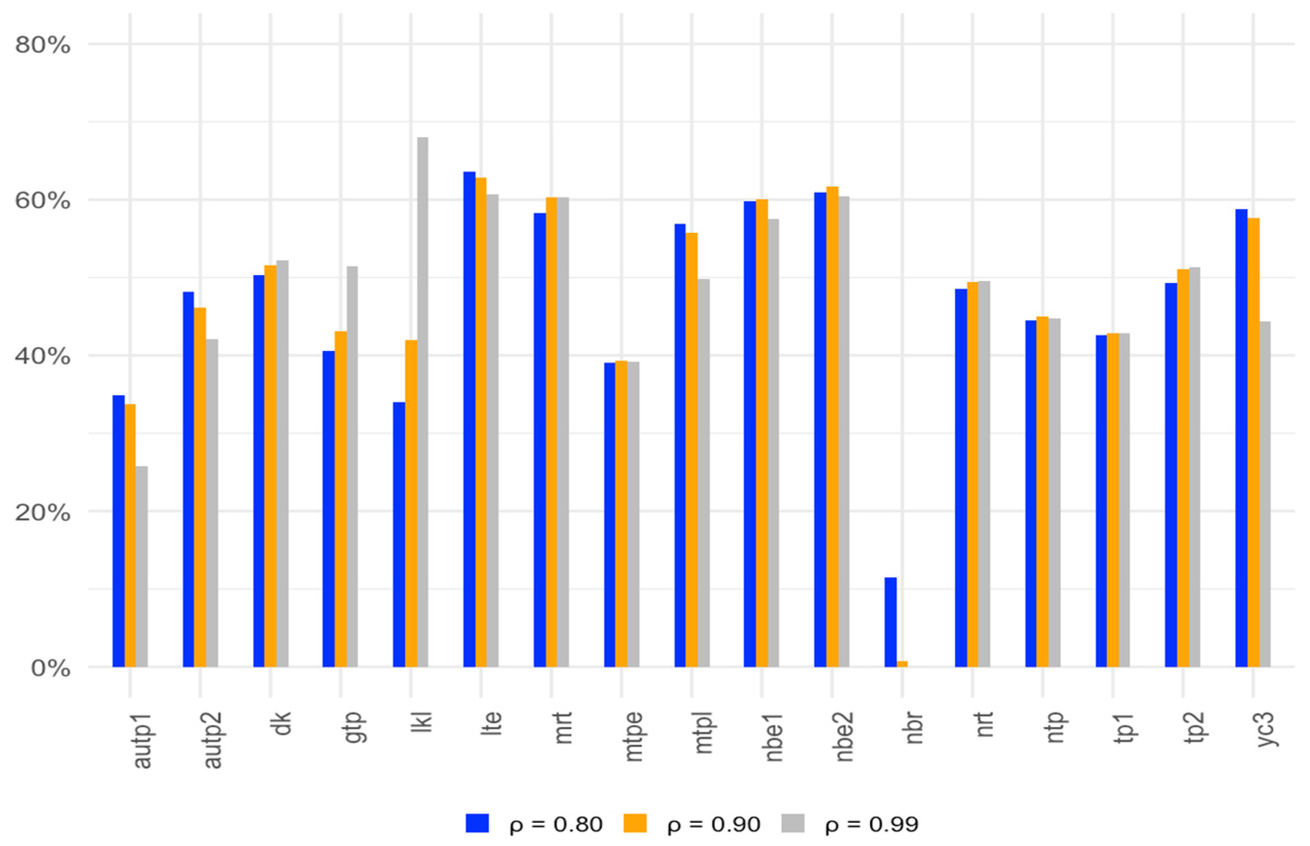
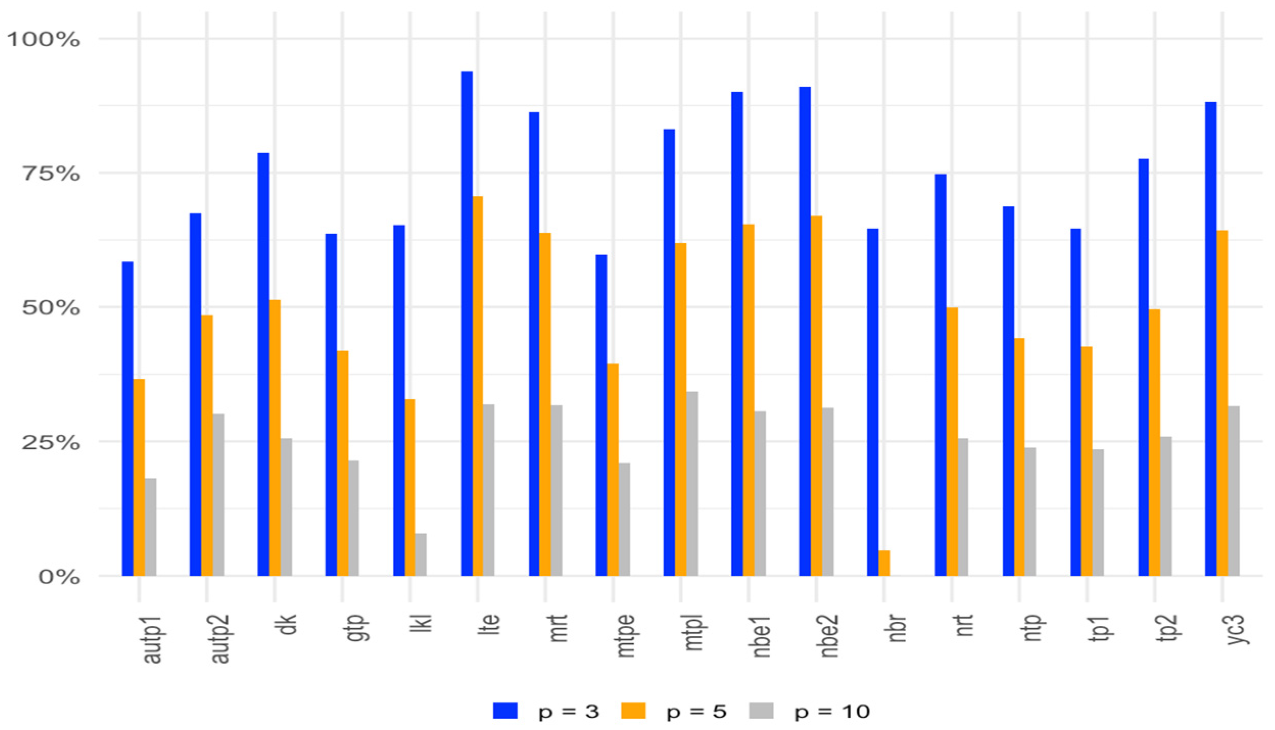
Figure 1, Figure 2 and Figure 3 show the average gain in power for two-parameter estimators over the OLS test for $\alpha =0.05$ with different correlation levels, sample sizes, and numbers of regressors.

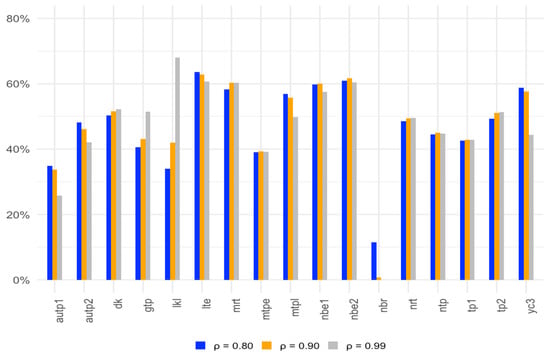
Figure 1. Average gain in power over the OLS test for α = 0.05 at correlation levels of 0.80, 0.90, and 0.99.

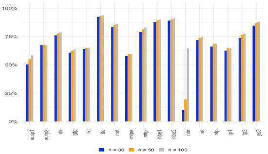
Figure 2. Average gain in power over the OLS test for α = 0.05 with sample sizes of 30, 50, and 100.

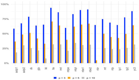
Figure 3. Average gain in power over the OLS test for α = 0.05 with 3, 5, and 10 parameters.

As we have only considered ${\sigma }^2=1$, we examine two additional values, ${\sigma }^2=5$ and 10, which are given in Table 8, Table 9 and Table 10.

Table 8. Statistical power for ${\mathit{\sigma }}^2=\mathbf{5}$ and 10 for $\mathit{\rho }=\mathbf{0.80}$.

p			3						10
n	30	30	50	50	100	100	30	30	50	50	100	100
${\mathit{\sigma }}^2$	5	10	5	10	5	10	5	10	5	10	5	10
OLS	0.1615	0.0997	0.1692	0.1067	0.1693	0.1132	0.0758	0.0604	0.0813	0.0616	0.086	0.0659
LTE	0.3626	0.1973	0.3907	0.2195	0.4015	0.2309	0.0716	0.054	0.0859	0.0613	0.0967	0.0701
NBE2	0.287	0.1553	0.3157	0.1725	0.3297	0.1839	0.0714	0.0538	0.0853	0.0611	0.0959	0.0697
YC3	0.2547	0.1343	0.2861	0.151	0.2993	0.1653	0.0732	0.0544	0.0902	0.0633	0.1031	0.0738
DK	0.257	0.1457	0.2791	0.1607	0.29	0.1724	0.0758	0.0594	0.083	0.0622	0.0891	0.0674
MRT	0.2636	0.1442	0.2906	0.1641	0.3039	0.1753	0.0701	0.0525	0.0859	0.0609	0.0979	0.0704
LKL	0.2539	0.1379	0.2738	0.1577	0.286	0.1735	0.0095	0.0051	0.0198	0.0129	0.0396	0.0309

Table 9. Statistical power for ${\mathit{\sigma }}^2=\mathbf{5}$ and 10 for $\mathit{\rho }=\mathbf{0.90}$.

p			3						10
n	30	30	50	50	100	100	30	30	50	50	100	100
${\mathit{\sigma }}^2$	5	10	5	10	5	10	5	10	5	10	5	10
OLS	0.1624	0.1031	0.1653	0.1027	0.1679	0.1085	0.0757	0.0582	0.0801	0.0651	0.0857	0.0667
LTE	0.4057	0.2237	0.4322	0.2307	0.4441	0.2467	0.0697	0.0513	0.0826	0.0636	0.0942	0.0696
NBE2	0.3556	0.1856	0.3813	0.1934	0.3979	0.2078	0.0697	0.0513	0.0825	0.0635	0.0941	0.0696
YC3	0.2851	0.1521	0.3111	0.1617	0.3276	0.1765	0.0713	0.0515	0.0845	0.0649	0.0964	0.0715
DK	0.3059	0.1717	0.3239	0.177	0.3346	0.1853	0.0753	0.0573	0.0813	0.0652	0.0884	0.0675
MRT	0.3401	0.18	0.3728	0.1923	0.3912	0.207	0.0685	0.0502	0.0828	0.0631	0.0954	0.0701
LKL	0.3881	0.2199	0.4074	0.2403	0.4179	0.2623	0.0239	0.0123	0.0359	0.0221	0.0593	0.0423

Table 10. Statistical power for ${\mathit{\sigma }}^2=\mathbf{5}$ and 10 for $\mathit{\rho }=\mathbf{0.99}$.

p			3						10
n	30	30	50	50	100	100	30	30	50	50	100	100
${\mathit{\sigma }}^2$	5	10	5	10	5	10	5	10	5	10	5	10
OLS	0.1641	0.1033	0.1641	0.1073	0.1694	0.111	0.0768	0.0591	0.0786	0.0648	0.0874	0.0678
LTE	0.4299	0.26	0.4615	0.2711	0.4855	0.2815	0.0677	0.0508	0.078	0.062	0.0914	0.0687
NBE2	0.4401	0.2632	0.4727	0.2777	0.4977	0.2908	0.0679	0.0509	0.0781	0.062	0.0915	0.0688
YC3	0.2395	0.1759	0.2747	0.1895	0.3101	0.2069	0.0638	0.0492	0.0748	0.0605	0.0893	0.0675
DK	0.3227	0.1993	0.3306	0.2066	0.3448	0.2119	0.0758	0.0574	0.0793	0.0645	0.089	0.0685
MRT	0.4959	0.2993	0.5279	0.3241	0.5508	0.3473	0.0663	0.0492	0.078	0.0614	0.0923	0.0689
LKL	0.6239	0.4448	0.6508	0.4957	0.6647	0.5095	0.0881	0.0786	0.1304	0.1218	0.1666	0.1476

For additional levels of variance, the results show the decrease in power with the increase in variance. They also result in higher power than the OLS estimator.

We also want to consider sample sizes of 200 and 300 so that we can determine the power for the test compared to the lower sample sizes which are given in Table 11, Table 12 and Table 13. For the power, we take the same procedure as that followed by Gokpinar and Ebegil (2016) [12] and choose $L=5$ to find the higher power.

Table 11. Statistical power for n = 200 and 300 and $\mathit{\rho }=0.80$.

p	3	3	5	5	10	10
n	200	300	200	300	200	300
OLS	0.8159	0.8216	0.6038	0.6017	0.3497	0.3483
LTE	0.9834	0.9858	0.8561	0.8598	0.4714	0.4721
NBE2	0.9747	0.9777	0.8342	0.8381	0.4634	0.4635
YC3	0.9613	0.9639	0.8112	0.815	0.4593	0.4593
DK	0.9098	0.9128	0.7014	0.7033	0.3804	0.3785
MRT	0.953	0.9571	0.8074	0.8088	0.4677	0.4672
LKL	0.7362	0.7398	0.4124	0.4176	0.1365	0.1474

Table 12. Statistical power for n = 200 and 300 and $\mathit{\rho }=0.90$.

p	3	3	5	5	10	10
n	200	300	200	300	200	300
OLS	0.8149	0.8198	0.6	0.6047	0.3473	0.3536
LTE	0.9846	0.9849	0.8512	0.853	0.4487	0.4555
NBE2	0.9793	0.9811	0.841	0.8418	0.4464	0.4534
YC3	0.9595	0.9643	0.8024	0.8056	0.4314	0.4394
DK	0.9187	0.9211	0.7067	0.7104	0.3735	0.3804
MRT	0.9637	0.9665	0.823	0.8224	0.4553	0.4632
LKL	0.8003	0.8035	0.5242	0.5306	0.2021	0.217

Table 13. Statistical power for n = 200 and 300 and $\mathit{\rho }=0.99$.

p	3	3	5	5	10	10
n	200	300	200	300	200	300
OLS	0.8171	0.8206	0.5988	0.6115	0.3492	0.3481
LTE	0.985	0.9841	0.8301	0.8389	0.4155	0.4171
NBE2	0.9831	0.9826	0.8292	0.8374	0.4165	0.4184
YC3	0.9459	0.9523	0.7561	0.7717	0.3968	0.399
DK	0.9303	0.9342	0.7003	0.7109	0.3671	0.3658
MRT	0.9737	0.9732	0.8259	0.8311	0.4272	0.4296
LKL	0.9309	0.9335	0.8142	0.8225	0.543	0.5516

As sample size increases to 200 and 300, the results suggest that the power increases with the increase in sample sizes. As the number of regressors increases, the power reduces while keeping the sample size constant.

We also introduce additional simulation scenarios where errors are drawn from alternative distributions—such as the t-distribution with a low degree of freedom in Table 14 and the exponential distribution with a rate of 1 in Table 15.

Table 14. Statistical power for ρ = 0.80 using errors from t-distribution.

p	3			5
n	10	20	30	10	20	30	20	30
OLS	0.3622	0.5199	0.5609	0.1728	0.3304	0.3604	0.162	0.1996
LTE	0.6885	0.8826	0.9102	0.2004	0.5611	0.6191	0.1533	0.234
NBE2	0.5577	0.8272	0.8675	0.1701	0.51	0.5755	0.1505	0.2294
YC3	0.4016	0.7678	0.8267	0.1243	0.474	0.5439	0.1512	0.23
DK	0.4393	0.6917	0.7372	0.1765	0.3878	0.4366	0.163	0.2099
MRT	0.4929	0.7641	0.8121	0.1643	0.4761	0.5446	0.1481	0.231
LKL	0.4569	0.5987	0.6219	0.0684	0.2597	0.2816	0.0264	0.0381

Table 15. Statistical power for ρ = 0.90 using errors from exponential distribution.

p	3			5
n	10	20	30	10	20	30	20	30
OLS	0.2728	0.3514	0.3606	0.1376	0.2226	0.2334	0.1162	0.1313
LTE	0.5647	0.7293	0.7594	0.1525	0.3513	0.3904	0.0972	0.1363
NBE2	0.4835	0.6897	0.7243	0.1362	0.3328	0.3706	0.0969	0.1358
YC3	0.2512	0.5703	0.6239	0.0836	0.2834	0.3272	0.0928	0.1322
DK	0.3893	0.5654	0.6026	0.1408	0.2581	0.2771	0.1144	0.1345
MRT	0.4157	0.6503	0.6871	0.1273	0.322	0.3659	0.0938	0.1363
LKL	0.4692	0.5931	0.6047	0.0615	0.2816	0.3039	0.0293	0.0504

4. Application to Real-Life Data

To illustrate the simulation results and findings of this paper, we analyze a pollution dataset which was originally published by McDoland and Schwing (1973) [45] in this section. These data model the total age-adjusted mortality rate for the years 1959–1961 across 201 Standard Metropolitan Statistical Areas (SMSAs), with the data sourced from Duffy and Carroll (1967) [46]. The dataset has 60 observations and 15 independent variables measuring demographic, socioeconomic, and environmental factors.

We consider the following model:

$$Y={\beta }_0+{\beta }_1{X}_1+{\beta }_2{X}_2+\cdots +{\beta }_{15}{X}_{15}+ϵ$$

where $Y$ = total age-adjusted mortality rate, $X_1$ = PREC (mean annual precipitation), $X_2$ = JANT (mean January temperature), $X_3$ = JULT (mean July temperature), $X_4$ = OVR65 (percent of population which is 65 years of age or over), $X_5$ = POPN (population per household), $X_6$ = EDUC (median school years), $X_7$ = HOUS (percent of housing units), $X_8$ = DENS (population per square mile), $X_9$ = NONW (percent of population which is non-white), $X_{10}$ = WWDRK (percent employment in white color occupation), $X_{11}$ = POOR (percent of families with low income), $X_{12}$ = HC (relative population potential of hydrocarbons), $X_{13}$ = NOX (relative population potential of oxides of nitrogen), $X_{14}$ = SOx (relative population potential of sulfur dioxide), and $X_{15}$ = HUMID (percent relative humidity).

Independent variables in this dataset exhibit high levels of correlation, or multicollinearity. For multicollinearity, we can use the variance inflation factor (VIF), calculated as

$$VI{F}_i={\displaystyle \frac{1}{1-R_i^2}},i=1,\dots ,p,$$

where $R_i^2$ is the multiple correlation coefficient obtained from regression of the explanatory variable. The VIF values are given in Table 16.

Table 16. Variance inflation factor.

Variable	VIF
PREC	4.113888
JANT	6.143551
JULT	3.967774
OVR65	7.470045
POPN	4.307618
EDUC	4.860538
HOUS	3.994781
DENS	1.658281
NONW	6.779599
WWDRK	2.841582
POOR	8.717068
HC	98.639935
NOX	104.982405
SOx	4.228929
HUMID	1.907092

Based on the VIF values, it can be seen that variables such as HC (98.64) and NOX (104.98) exhibit a high level of multicollinearity; therefore, we can state that there is a dependency among explanatory variables.

To detect multicollinearity, we obtain the condition number value calculated as $CN={\left({\displaystyle \frac{largest eigen value}{smallest eigenvalue}}\right)}^{1/2}=\mathrm{35,406.49}$. We can see that the CN value is 35,406.49, which is more than 10, so it confirms that severe multicollinearity among the variables exists.

To evaluate the significance of the regression coefficients, we want to test the null hypothesis. We calculate the p values as $p=2\times P(t_{n-k-1}>|t_{\alpha }\left|\right)$. If $p<\alpha$ (typically), we reject the null hypothesis, indicating that the regression coefficients are statistically significant. In Table 17, we present the parameter estimates, standard errors, and p-values for each regression coefficient.

Table 17. Results of pollution data analysis comparing two-parameter models with OLS.

		OLS			LTE			NBE2
	Coef	SE	p-value	Coef	SE	p-value	Coef	SE	p-value
PREC	1.175	1.06	0.274	1.036	1.373	0.455	1.209	1.078	0.268
JANT	−1.516	1.291	0.247	−1.328	1.672	0.431	−1.789	1.251	0.16
JULT	1.319	1.819	0.472	1.164	2.356	0.624	1.6	1.79	0.376
OVR65	11.184	8.008	0.17	9.822	10.369	0.349	10.381	8.225	0.214
POPN	128.036	45.007	0.007	112.444	58.28	0.06	113.282	39.854	0.007
EDUC	−1.463	13.112	0.912	−1.284	16.979	0.94	−2.157	14.285	0.881
HOUS	1.221	1.996	0.544	1.078	2.585	0.679	1.591	1.985	0.427
DENS	0.007	0.005	0.108	0.032	0.006	0.001	0.007	0.005	0.122
NONW	4.13	1.55	0.011	3.628	2.008	0.078	4.089	1.593	0.014
WWDRK	0.447	1.936	0.818	0.397	2.507	0.875	0.463	2.03	0.821
POOR	1.886	3.73	0.616	1.658	4.83	0.733	2.445	3.711	0.513
HC	−0.373	0.568	0.514	−0.328	0.736	0.658	−0.382	0.573	0.509
NOX	0.874	1.169	0.458	0.768	1.514	0.614	0.907	1.182	0.447
SOx	0.16	0.171	0.357	0.14	0.222	0.532	0.154	0.174	0.381
HUMID	1.915	1.264	0.137	1.687	1.637	0.308	2.127	1.242	0.094
		YC3			DK			MRT
	Coef	SE	p-value	Coef	SE	p-value	Coef	SE	p-value
PREC	2.05	0.799	0.014	1.222	1.058	0.254	1.461	1.065	0.177
JANT	−3.199	0.788	0.001	−1.769	1.237	0.16	−2.996	1.06	0.007
JULT	4.357	1.098	0.001	1.589	1.777	0.376	2.908	1.671	0.089
OVR65	1.449	1.191	0.23	10.353	7.898	0.197	6.262	7.474	0.407
POPN	0.65	0.151	0.001	113.923	40.077	0.007	45.208	16.413	0.009
EDUC	0.155	0.727	0.832	−1.714	12.99	0.896	−2.595	11.723	0.826
HOUS	3.165	1.082	0.005	1.538	1.938	0.432	3.054	1.747	0.087
DENS	0.007	0.005	0.128	0.007	0.005	0.114	0.007	0.005	0.153
NONW	3.193	0.883	0.001	4.076	1.546	0.012	3.807	1.543	0.018
WWDRK	0.166	1.195	0.89	0.427	1.928	0.826	0.298	1.871	0.874
POOR	4.294	1.563	0.009	2.401	3.652	0.514	4.899	3.443	0.162
HC	−0.452	0.517	0.386	−0.379	0.568	0.509	−0.401	0.583	0.495
NOX	1.173	1.036	0.264	0.899	1.169	0.446	1.016	1.194	0.399
SOx	0.161	0.157	0.311	0.157	0.171	0.365	0.145	0.173	0.409
HUMID	3.835	0.928	0.001	2.115	1.23	0.093	3.084	1.138	0.01
		LKL
	Coef	SE	p-value
PREC	1.639	1.117	0.149
JANT	−3.947	1.07	0.001
JULT	3.924	1.731	0.028
OVR65	3.134	7.676	0.685
POPN	−7.781	3.22	0.02
EDUC	−3.455	11.6	0.767
HOUS	4.24	1.779	0.022
DENS	0.006	0.005	0.206
NONW	3.606	1.609	0.03
WWDRK	0.215	1.924	0.912
POOR	6.833	3.559	0.061
HC	−0.42	0.615	0.499
NOX	1.108	1.257	0.383
SOx	0.134	0.182	0.464
HUMID	3.832	1.173	0.002

Notes: Coef: regression coefficient; SE: standard error.

Based on the previous simulation results for type I errors and test power, certain two-parameter estimators, such as LTE, NBE2, MRT, and LKL, demonstrate higher power than others compared to OLS. Additionally, YC3 and DK also show improved power. Therefore, we want to evaluate the performance of these estimators with the real-life data affected by multicollinearity.

The corresponding parameter estimates, standard errors, and p-values are presented in Table 17. From the table, we can see that variables PREC, JANT, JULT, HOUS, POOR, and HUMID are not significant at the alpha level of 0.05 for the OLS estimator. However, under the YC3 estimator, all of these variables are statistically significant. Also, for the MRT estimator, the variables JANT, JULT, and HUMID are significant, and for the LKL estimator, the variables JANT, JULT, HOUS, POOR, and HUMID are significant.

Furthermore, the highest VIF variables, HC and NOX, are not significant under any estimation method. But some other high VIF variables, such as JANT and POOR, are significant under specific estimators. Also, the NONW variable is statistically significant across all of them, indicating its consistent impact. Therefore, we observe that all of the estimators perform better than the OLS estimator, but among them YC3 (Yang and Chang estimator) performs better than the other estimators on these data.

Another example we use are “body data” which can be found in the textbook Biostatistics for the Biological and Health Sciences, 2nd edition by Triola et al. (2006) [47]. These data are also available at “www.triolastats.com (accessed on 24 February 2015)”. The dataset consists of body and exam measurements for 300 subjects. The outcome variable for our model is HDL cholesterol (mg/dL). The explanatory variables are x1: weight (kg), x2: height (cm), x3: waist circumference (cm), x4: arm circumference (cm), and x5: BMI (Body Mass Index). The VIF values for the body dataset are given in Table 18.

Table 18. VIF for body data.

Variable	VIF
x1—weight (kg)	89.942300
x2—height (cm)	19.724450
x3—waist circumference (cm)	8.249625
x4—arm circumference (cm)	5.793885
x5—BMI	77.377840

There is evidence of multicollinearity in the data, as evidenced by several of the variance inflation factors (VIFs) being greater than 10 (see the paper by Ozkale and Kacıranlar (2007) [19], which is in practice considered the threshold for multicollinearity.

We can also see that the condition number is 143.6735, which also indicates that there is severe multicollinearity.

From Table 19, we can see that variable x3 is significant and variable x4 has a p-value of around 0.06 for most models, including the OLS estimator. Using the YC3 estimator, both x3 and x4 variables are highly non-significant; the MRT estimator shows non-significant results for the x4 variable. So, YC3 and MRT estimators provide better results for multicollinear independent variables.

Table 19. Results of body data analysis.

		OLS			LTE			NBE2
	Coef	SE	p-value	Coef	SE	p-value	Coef	SE	p-value
x1	−0.6869	0.1024	0.001	−0.6595	0.0984	0.001	−0.6839	0.1018	0.001
x2	0.5866	0.0552	0.001	0.5741	0.0531	0.001	0.5771	0.0535	0.001
x3	−0.4446	0.1443	0.0023	−0.4231	0.1384	0.0024	−0.4233	0.1416	0.003
x4	−0.7695	0.4189	0.0672	−0.7353	0.4012	0.0678	−0.7069	0.4041	0.0813
x5	2.791	0.4491	0.001	2.6719	0.4301	0.001	2.693	0.4317	0.001
		YC3			DK			MRT
	Coef	SE	p-value	Coef	SE	p-value	Coef	SE	p-value
x1	−0.6218	0.0937	0.001	−0.6844	0.1019	0.001	−0.6773	0.1008	0.001
x2	0.4717	0.0366	0.001	0.5777	0.0536	0.001	0.556	0.0498	0.001
x3	−0.1627	0.1109	0.1436	−0.4248	0.1418	0.003	−0.3758	0.1357	0.006
x4	−0.0778	0.2349	0.7408	−0.7096	0.4051	0.0809	−0.5674	0.3716	0.1278
x5	1.5139	0.2348	0.001	2.6998	0.4328	0.001	2.4746	0.3931	0.001
		LKL
	Coef	SE	p-value
x1	−0.6866	0.1023	0.001
x2	0.5854	0.055	0.001
x3	−0.4418	0.1439	0.0023
x4	−0.7608	0.417	0.0691
x5	2.778	0.4468	0.001

5. Concluding Remarks

In this paper, we examined various test statistics derived from two-parameter estimators to address multicollinearity issues when testing regression coefficients within a linear regression model. We conducted a simulation study under several conditions and compared these test statistics empirically, evaluating their performance in terms of empirical size and power. Our findings show that several two-parameter estimators consistently outperformed other tests, demonstrating their effectiveness in managing multicollinearity and producing more reliable results. Specifically, the LTE, NBE2, YC3, MRT, and LKL estimators exhibited higher power than the others. These results provide valuable insights for selecting appropriate test statistics for regression coefficient testing in multicollinearity settings, contributing to the refinement of regression analysis methodology and more accurate inference for practitioners. Finally, we analyzed a pollution dataset and body data to illustrate the findings of this paper, which supported the simulation results to some extent. We can suggest that some estimators like YC3 and MRT work better than other estimators and OLS when there is multicollinearity. They can help to determine which variables are significant and perform better than OLS in the presence of multicollinearity.

In the future, we can use these estimators to test parameters for other types of regression models, like logistic and Poisson regression, and in more complex settings like mixed models. Another area of research is to investigate hypothesis testing for survival regression models like Weibull, exponential, and Cox Proportional Hazards models in the presence of multicollinearity.

References

- Kibria, B.M.G. Performance of some new ridge regression estimators. Commun. Stat. Simul. Comput. 2003, 32, 419–435. [Google Scholar] [CrossRef]
- Hoerl, A.E.; Kennard, R.W. Ridge regression: Biased estimation for nonorthogonal problems. Technometrics 1970, 12, 55–67. [Google Scholar] [CrossRef]
- Ehsanes Saleh, A.M.; Kibria, B.M.G. Performance of some new preliminary test ridge regression estimators and their properties. Commun. Stat. Theory Methods 1993, 22, 2747–2764. [Google Scholar] [CrossRef]
- Alheety, M.I.; Nayem, H.M.; Kibria, B.M.G. An Unbiased Convex Estimator Depending on Prior Information for the Classical Linear Regression Model. Stats 2025, 8, 16. [Google Scholar] [CrossRef]
- Dawoud, I.; Kibria, B.M.G. A new biased estimator to combat the multicollinearity of the Gaussian linear regression model. Stats 2020, 3, 526–541. [Google Scholar] [CrossRef]
- Hoque, M.A.; Kibria, B.M.G. Some one and two parameter estimators for the multicollinear gaussian linear regression model: Simulations and applications. Surv. Math. Its Appl. 2023, 18, 183–221. [Google Scholar]
- Hoque, M.A.; Kibria, B.M.G. Performance of some estimators for the multicollinear logistic regression model: Theory, simulation, and applications. Res. Stat. 2024, 2, 2364747. [Google Scholar] [CrossRef]
- Nayem, H.M.; Aziz, S.; Kibria, B.M.G. Comparison among Ordinary Least Squares, Ridge, Lasso, and Elastic Net Estimators in the Presence of Outliers: Simulation and Application. Int. J. Stat. Sci. 2024, 24, 25–48. [Google Scholar] [CrossRef]
- Yasmin, N.; Kibria, B.M.G. Performance of Some Improved Estimators and their Robust Versions in Presence of Multicollinearity and Outliers. Sankhya B 2025, 2025, 1–47. [Google Scholar] [CrossRef]
- Halawa, A.M.; El Bassiouni, M.Y. Tests of regression coefficients under ridge regression models. J. Stat. Comput. Simul. 2000, 65, 341–356. [Google Scholar] [CrossRef]
- Cule, E.; Vineis, P.; De Iorio, M. Significance testing in ridge regression for genetic data. BMC Bioinform. 2011, 12, 372. [Google Scholar] [CrossRef]
- Gökpınar, E.; Ebegil, M. A study on tests of hypothesis based on ridge estimator. Gazi Univ. J. Sci. 2016, 29, 769–781. [Google Scholar]
- Kibria, B.M.G.; Banik, S. A simulation study on the size and power Properties of some ridge regression Tests. Appl. Appl. Math. Int. J. (AAM) 2019, 14, 7. [Google Scholar]
- Perez-Melo, S.; Kibria, B.M.G. On some test statistics for testing the regression coefficients in presence of multicollinearity: A simulation study. Stats 2020, 3, 40–55. [Google Scholar] [CrossRef]
- Ullah, M.I.; Aslam, M.; Altaf, S. lmridge: A Comprehensive R Package for Ridge Regression. R J. 2018, 10, 326. [Google Scholar] [CrossRef]
- Perez-Melo, S.; Bursac, Z.; Kibria, B.M.G. Comparison of Test Statistics for Testing the Regression Coefficients in the OLS, Ridge, Liu and Kibria-Lukman Linear Regression Model: A Simulation Study. In JSM Proceedings, Biometrics Section; American Statistical Association: Alexandria, VA, USA, 2022; pp. 59–80. [Google Scholar]
- Yang, H.; Chang, X. A new two-parameter estimator in linear regression. Commun. Stat. Theory Methods 2010, 39, 923–934. [Google Scholar] [CrossRef]
- Liu, K. Using Liu-type estimator to combat collinearity. Commun. Stat. Theory Methods 2003, 32, 1009–1020. [Google Scholar] [CrossRef]
- Özkale, M.R.; Kaciranlar, S. The restricted and unrestricted two-parameter estimators. Commun. Stat. Theory Methods 2007, 36, 2707–2725. [Google Scholar] [CrossRef]
- Hoerl, A.E.; Kennard, R.W.; Baldwin, K.F. Ridge regression: Some simulations. Commun. Stat. Theory Methods 1975, 4, 105–123. [Google Scholar] [CrossRef]
- Sakallıoğlu, S.; Kaçıranlar, S. A new biased estimator based on ridge estimation. Stat. Pap. 2008, 49, 669–689. [Google Scholar] [CrossRef]
- Wu, J.; Yang, H. Efficiency of an almost unbiased two-parameter estimator in linear regression model. Statistics 2013, 47, 535–545. [Google Scholar] [CrossRef]
- Wu, J. An Unbiased Two-Parameter Estimation with Prior Information in Linear Regression Model. Sci. World J. 2014, 1, 206943. [Google Scholar] [CrossRef] [PubMed]
- Dorugade, A.V. A modified two-parameter estimator in linear regression. Stat. Transit. New Ser. 2014, 15, 23–36. [Google Scholar] [CrossRef]
- Arumairajan, S.; Wijekoon, P. Modified almost unbiased Liu estimator in linear regression model. Commun. Math. Stat. 2017, 5, 261–276. [Google Scholar] [CrossRef]
- Lukman, A.F.; Adewuyi, E.; Oladejo, N.; Olukayode, A. Modified almost unbiased two-parameter estimator in linear regression model. In IOP Conference Series: Materials Science and Engineering; IOP Publishing: Bristol, UK, 2019; Volume 640, p. 012119. [Google Scholar]
- Lukman, A.F.; Ayinde, K.; Siok Kun, S.; Adewuyi, E.T. A modified new two-parameter estimator in a linear regression model. Model. Simul. Eng. 2019, 2019, 6342702. [Google Scholar] [CrossRef]
- Lukman, A.F.; Ayinde, K.; Binuomote, S.; Clement, O.A. Modified ridge-type estimator to combat multicollinearity: Application to chemical data. J. Chemom. 2019, 33, e3125. [Google Scholar] [CrossRef]
- Zeinal, A. Generalized two-parameter estimator in linear regression model. J. Math. Model. 2020, 8, 157–176. [Google Scholar] [CrossRef]
- Üstündağ Şiray, G.; Toker, S.; Özbay, N. Defining a two-parameter estimator: A mathematical programming evidence. J. Stat. Comput. Simul. 2021, 91, 2133–2152. [Google Scholar] [CrossRef]
- Abidoye, A.O.; Ajayi, I.M.; Adewale, F.L.; Ogunjobi, J.O. Unbiased Modified Two-Parameter Estimator for the Linear Regression Model. J. Sci. Res. 2022, 14, 785–795. [Google Scholar] [CrossRef]
- Ahmad, S.; Aslam, M. Another proposal about the new two-parameter estimator for linear regression model with correlated regressors. Commun. Stat. Simul. Comput. 2022, 51, 3054–3072. [Google Scholar] [CrossRef]
- Aslam, M.; Ahmad, S. The modified Liu-ridge-type estimator: A new class of biased estimators to address multicollinearity. Commun. Stat. Simul. Comput. 2022, 51, 6591–6609. [Google Scholar] [CrossRef]
- Dawoud, I.; Lukman, A.F.; Haadi, A.R. A new biased regression estimator: Theory, simulation and application. Sci. Afr. 2022, 15, e01100. [Google Scholar] [CrossRef]
- Idowu, J.I.; Oladapo, O.J.; Owolabi, A.T.; Ayinde, K. On the biased Two-Parameter Estimator to Combat Multicollinearity in Linear Regression Model. Afr. Sci. Rep. 2022, 1, 188–204. [Google Scholar] [CrossRef]
- Owolabi, A.T.; Ayinde, K.; Idowu, J.I.; Oladapo, O.J.; Lukman, A.F. A new two-parameter estimator in the linear regression model with correlated regressors. J. Stat. Appl. Probab. 2022, 11, 185–201. [Google Scholar]
- Owolabi, A.T.; Ayinde, K.; Alabi, O.O. A new ridge-type estimator for the linear regression model with correlated regressors. Concurr. Comput. Pract. Exp. 2022, 34, e6933. [Google Scholar] [CrossRef]
- Owolabi, A.T.; Ayinde, K.; Alabi, O.O. A Modified Two Parameter Estimator with Different Forms of Biasing Parameters in the Linear Regression Model. Afr. Sci. Rep. 2022, 1, 212–228. [Google Scholar] [CrossRef]
- Abonazel, M.R. New modified two-parameter Liu estimator for the Conway–Maxwell Poisson regression model. J. Stat. Comput. Simul. 2023, 93, 1976–1996. [Google Scholar] [CrossRef]
- Abdelwahab, M.M.; Abonazel, M.R.; Hammad, A.T.; El-Masry, A.M. Modified Two-Parameter Liu Estimator for Addressing Multicollinearity in the Poisson Regression Model. Axioms 2024, 13, 46. [Google Scholar] [CrossRef]
- Idowu, J.I.; Oladapo, O.J.; Owolabi, A.T.; Ayinde, K.; Akinmoju, O. Combating multicollinearity: A new two-parameter approach. Nicel Bilim. Derg. 2023, 5, 90–116. [Google Scholar] [CrossRef]
- Kibria, B.M.G.; Lukman, A.F. A new ridge-type estimator for the linear regression model: Simulations and applications. Scientifica 2020, 2020, 9758378. [Google Scholar] [CrossRef]
- Khan, M.S.; Ali, A.; Suhail, M.; Kibria, B.M.G. On some two parameter estimators for the linear regression models with correlated predictors: Simulation and application. Commun. Stat. Simul. Comput. 2024, 2024, 1–15. [Google Scholar] [CrossRef]
- R Core Team. _R: A Language and Environment for Statistical Computing_; R Foundation for Statistical Computing: Vienna, Austria, 2024; Available online: https://www.R-project.org/ (accessed on 11 August 2024).
- McDonald, G.C.; Schwing, R.C. Instabilities of regression estimates relating air pollution to mortality. Technometrics 1973, 15, 463–481. [Google Scholar] [CrossRef]
- Duffy, E.A.; Carroll, R.E. United States Metropolitan Mortality, 1959–1961; PHS Publication No. 1967, 999-AP-39; U.S. Public Health Service, National Center for Air Pollution Control: Philadelphia, PA, USA, 1967.
- Triola, M.M.; Triola, M.F.; Roy, J.A. Biostatistics for the Biological and Health Sciences; Pearson Addison-Wesley: Boston, MA, USA, 2006. [Google Scholar]
Disclaimer/Publisher’s Note: The statements, opinions and data contained in all publications are solely those of the individual author(s) and contributor(s) and not of MDPI and/or the editor(s). MDPI and/or the editor(s) disclaim responsibility for any injury to people or property resulting from any ideas, methods, instructions or products referred to in the content. |
© 2025 by the authors. Licensee MDPI, Basel, Switzerland. This article is an open access article distributed under the terms and conditions of the Creative Commons Attribution (CC BY) license (https://creativecommons.org/licenses/by/4.0/).